Communication Networks Sanjay K. Bose Lecture Set IV LANs and Media Access Control (MAC)

Welcome message from author
This document is posted to help you gain knowledge. Please leave a comment to let me know what you think about it! Share it to your friends and learn new things together.
Transcript
Communication Networks
Sanjay K. Bose
Lecture Set IV
LANs and Media Access Control (MAC)
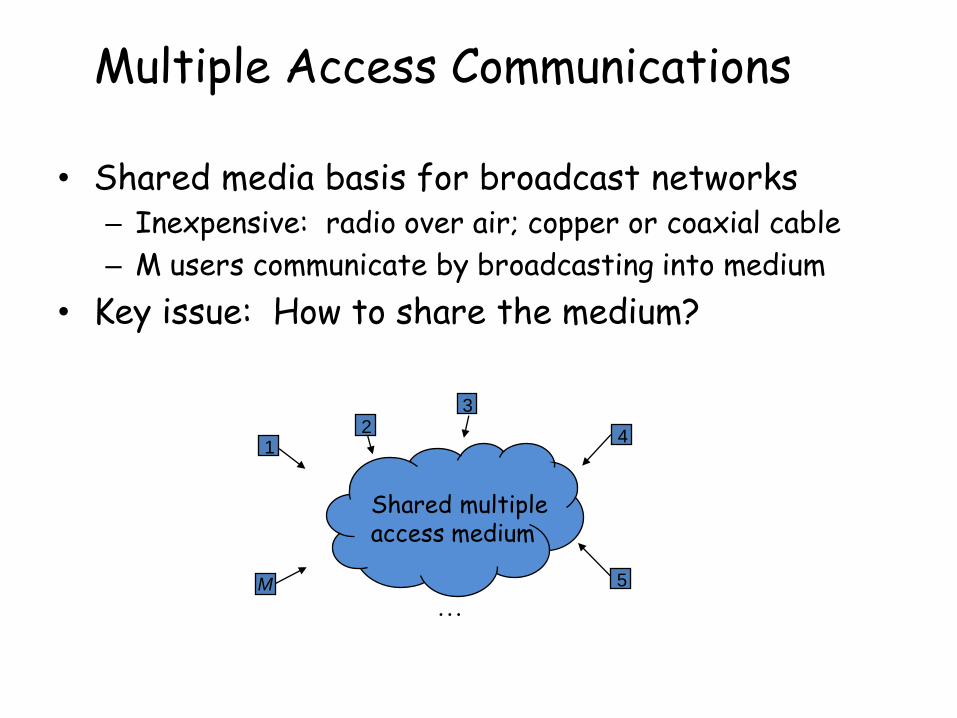
Multiple Access Communications
• Shared media basis for broadcast networks – Inexpensive: radio over air; copper or coaxial cable
– M users communicate by broadcasting into medium
• Key issue: How to share the medium?
1 2
3
4
5 M
Shared multiple access medium

Static channelization
Dynamic medium access control
Scheduling Random Access
Approaches to Media Sharing
Partition medium
Dedicated allocation to users
Used in Satellite Transmissions and
Cellular Telephony
Polling: take turns
Request for slot in transmission schedule
Used in Token Ring
Wireless LANs
Loose coordination
Send, wait, retry if necessary
Used in Aloha and
Ethernet

Random Access Protocols
When node has packet to send transmit at full channel data rate R.
no a priori coordination among nodes
two or more transmitting nodes ➜ “collision”,
random access MAC protocol specifies: how to detect collisions
how to recover from collisions (e.g., via delayed retransmissions)
Examples of random access MAC protocols: slotted ALOHA
ALOHA
CSMA, CSMA/CD, CSMA/CA

Pure ALOHA
When frame first arrives, transmit immediately and wait for ACK
If ACK is received, frame transmission was successful
If ACK is not received, wait for random time and try transmission again; repeat this until frame is successfully transmitted
In example shown, all frames are of unit length. Node i’s frame is successful if no other transmission starts between (t0-1, t0) or
between (t0, t0+1)
ACK and frames can share the same channel or the frames can be sent on a “forward” channel while the ACKs are sent on a “reverse” channel
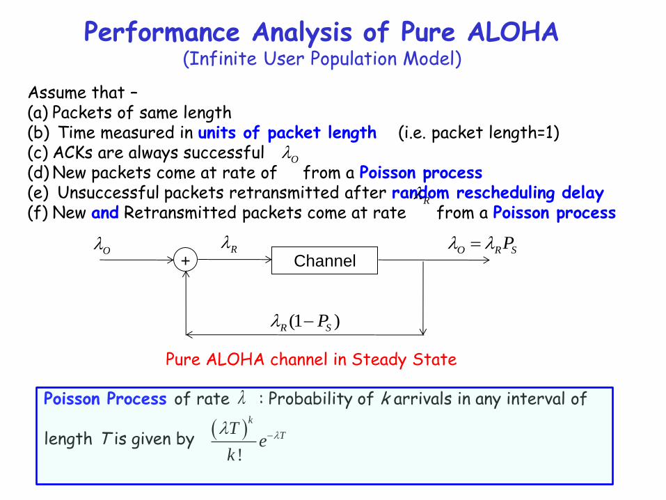
Poisson Process of rate : Probability of k arrivals in any interval of length T is given by
!
k
TT
ek
Performance Analysis of Pure ALOHA (Infinite User Population Model)
Assume that – (a) Packets of same length (b) Time measured in units of packet length (i.e. packet length=1) (c) ACKs are always successful (d) New packets come at rate of from a Poisson process (e) Unsuccessful packets retransmitted after random rescheduling delay (f) New and Retransmitted packets come at rate from a Poisson process
O
R
Channel + O R
O R SP
(1 )R SP
Pure ALOHA channel in Steady State
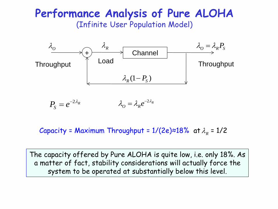
Performance Analysis of Pure ALOHA (Infinite User Population Model)
Channel + O R
O R SP
(1 )R SP
2 R
SP e
2 R
O Re
Throughput Throughput Load
Capacity = Maximum Throughput = 1/(2e)≈18% at = 1/2 R
The capacity offered by Pure ALOHA is quite low, i.e. only 18%. As a matter of fact, stability considerations will actually force the
system to be operated at substantially below this level.
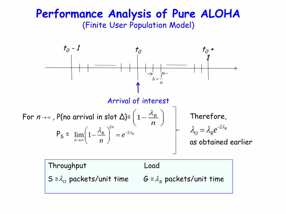
Performance Analysis of Pure ALOHA (Finite User Population Model)
t0 t0 + 1
t0 - 1
1
n
For n , P{no arrival in slot Δ}= PS =
1 R
n
Arrival of interest
2
2lim 1 R
n
R
ne
n
Therefore, as obtained earlier
2 R
O Re
Throughput Load
S = packets/unit time G = packets/unit time
OR

Throughput of ALOHA
G
success GeGPS 2
0
0.02
0.04
0.06
0.08
0.1
0.12
0.14
0.16
0.18
0.2
0
0.00
78125
0.01
5625
0.03
125
0.06
25
0.12
50.
25 0.5 1 2 4
G
S
Collisions are means for coordinating access
Max throughput is Smax= 1/2e (18.4%)
Bimodal behavior:
Small G, S≈G
Large G, S↓0
Collisions can snowball and drop throughput to zero
e-2 = 0.184
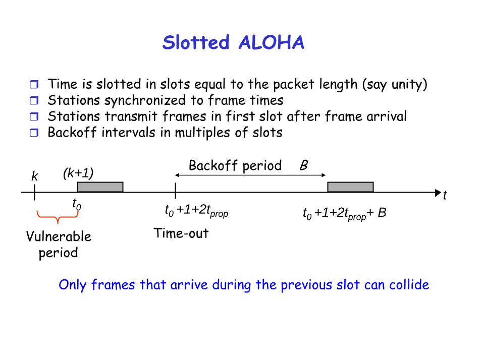
Slotted ALOHA
Time is slotted in slots equal to the packet length (say unity) Stations synchronized to frame times Stations transmit frames in first slot after frame arrival Backoff intervals in multiples of slots
t
(k+1) k
t0 +1+2tprop+ B
Vulnerable period
Time-out
Backoff period B
t0 +1+2tprop
Only frames that arrive during the previous slot can collide
t0
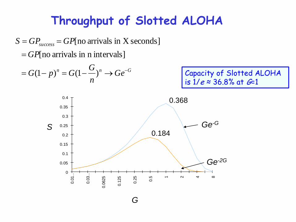
Throughput of Slotted ALOHA
Gnn
success
Gen
GGpG
GP
GPGPS
)1()1(
intervals]n in arrivals no[
seconds] Xin arrivals no[
0
0.05
0.1
0.15
0.2
0.25
0.3
0.35
0.4
0.0
1…
0.0
3…
0.0
625
0.1
25
0.2
5
0.5 1 2 4 8
Ge-G
Ge-2G
G
S 0.184
0.368
Capacity of Slotted ALOHA is 1/e ≈ 36.8% at G=1
Discrete-Time Markov Chain Analysis for Slotted ALOHA
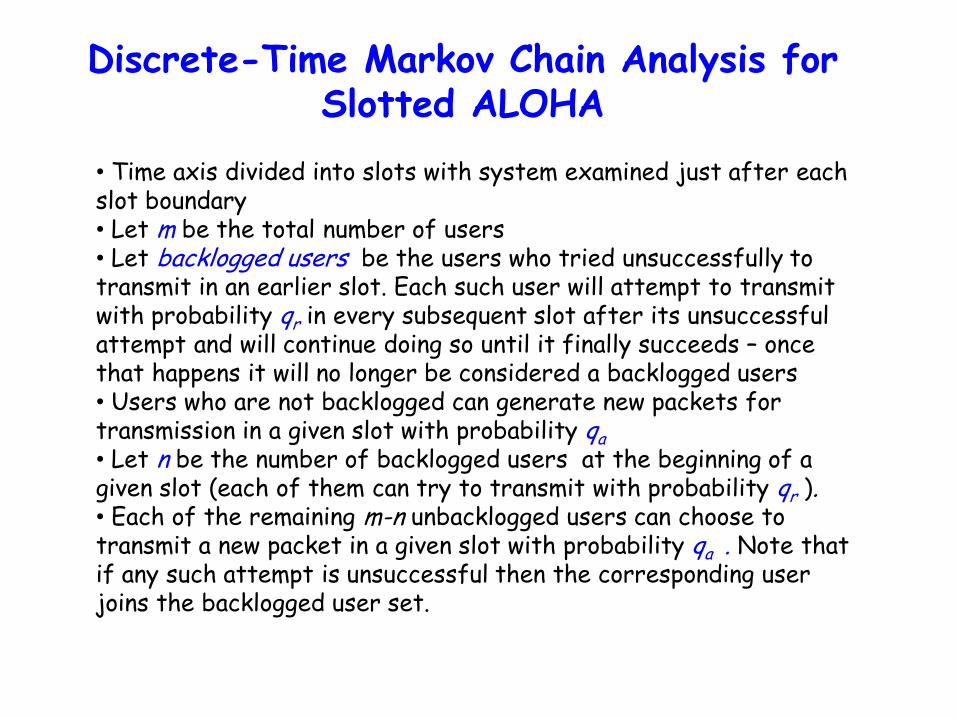
• Time axis divided into slots with system examined just after each slot boundary • Let m be the total number of users • Let backlogged users be the users who tried unsuccessfully to transmit in an earlier slot. Each such user will attempt to transmit with probability qr in every subsequent slot after its unsuccessful attempt and will continue doing so until it finally succeeds – once that happens it will no longer be considered a backlogged users • Users who are not backlogged can generate new packets for transmission in a given slot with probability qa • Let n be the number of backlogged users at the beginning of a given slot (each of them can try to transmit with probability qr ). • Each of the remaining m-n unbacklogged users can choose to transmit a new packet in a given slot with probability qa . Note that if any such attempt is unsuccessful then the corresponding user joins the backlogged user set.
Discrete-Time Markov Chain Analysis for Slotted ALOHA
p14
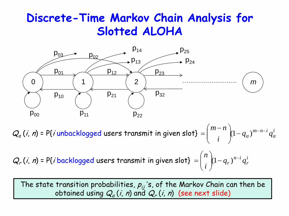
Qa (i, n) = P{i unbacklogged users transmit in given slot}
Qr (i, n) = P{i backlogged users transmit in given slot}
ia
inma qq
i
nm
)1(
ir
inr qq
i
n
)1(
The state transition probabilities, pij ‘s, of the Markov Chain can then be obtained using Qa (i, n) and Qr (i, n) (see next slide)
m 1 2
p22 p00 p11
p01
p10
p02
p12
p03 p13
p21
p23
p32
p24
p25
0
Discrete-Time Markov Chain Analysis for Slotted ALOHA
1),1(),0(
0)],1(1)[,0(),0(),1(
1)],0(1)[,1(
2),(,
inQnQ
inQnQnQnQ
inQnQ
nminiQp
ra
rara
ra
ainn
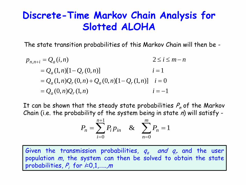
The state transition probabilities of this Markov Chain will then be -
It can be shown that the steady state probabilities Pn of the Markov Chain (i.e. the probability of the system being in state n) will satisfy -
m
n
n
n
i
inin PpPP
0
1
0
1&
Given the transmission probabilities, qa and qr and the user population m, the system can then be solved to obtain the state probabilities, Pi for i=0,1,…..,m
Discrete-Time Markov Chain Analysis for Slotted ALOHA
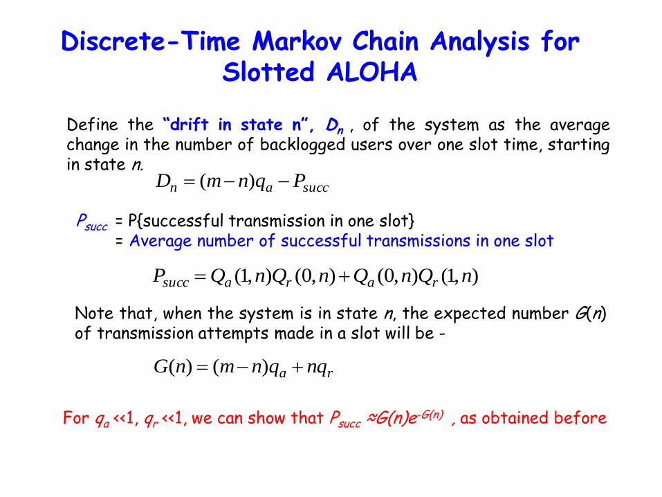
Define the “drift in state n”, Dn , of the system as the average change in the number of backlogged users over one slot time, starting in state n.
succan PqnmD )(
Psucc = P{successful transmission in one slot} = Average number of successful transmissions in one slot
),1(),0(),0(),1( nQnQnQnQP rarasucc
Note that, when the system is in state n, the expected number G(n) of transmission attempts made in a slot will be -
ra nqqnmnG )()(
For qa <<1, qr <<1, we can show that Psucc ≈G(n)e-G(n) , as obtained before
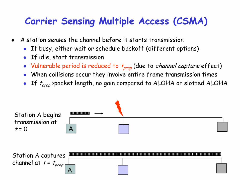
Carrier Sensing Multiple Access (CSMA)
A
Station A begins transmission at t = 0
A
Station A captures channel at t = tprop
A station senses the channel before it starts transmission
If busy, either wait or schedule backoff (different options)
If idle, start transmission
Vulnerable period is reduced to tprop (due to channel capture effect)
When collisions occur they involve entire frame transmission times
If tprop >packet length, no gain compared to ALOHA or slotted ALOHA
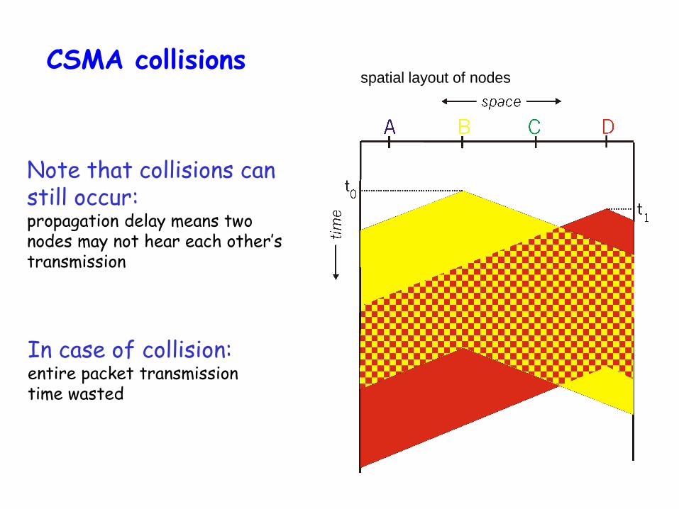
CSMA collisions
Note that collisions can still occur: propagation delay means two nodes may not hear each other’s transmission
In case of collision: entire packet transmission time wasted
spatial layout of nodes
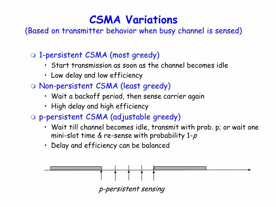
1-persistent CSMA (most greedy) • Start transmission as soon as the channel becomes idle
• Low delay and low efficiency
Non-persistent CSMA (least greedy) • Wait a backoff period, then sense carrier again
• High delay and high efficiency
p-persistent CSMA (adjustable greedy) • Wait till channel becomes idle, transmit with prob. p; or wait one
mini-slot time & re-sense with probability 1-p
• Delay and efficiency can be balanced
CSMA Variations (Based on transmitter behavior when busy channel is sensed)
p-persistent sensing
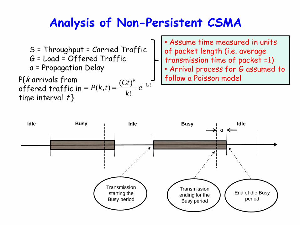
Analysis of Non-Persistent CSMA
S = Throughput = Carried Traffic G = Load = Offered Traffic a = Propagation Delay
• Assume time measured in units of packet length (i.e. average transmission time of packet =1) • Arrival process for G assumed to follow a Poisson model
Busy Busy Idle Idle Idle
Transmission
starting the
Busy period
Transmission
ending for the
Busy period
End of the Busy
period
a
Gtk
ek
GttkP
!
)(),(
P{k arrivals from offered traffic in time interval t }
Analysis of Non-Persistent CSMA
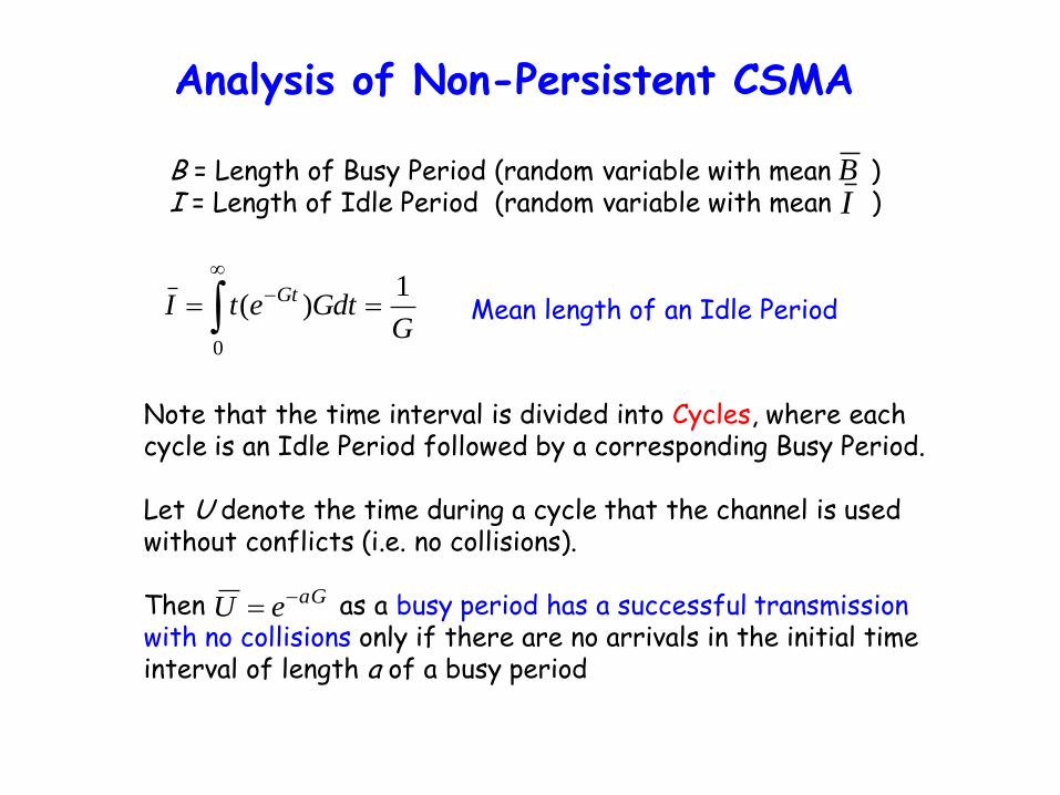
B = Length of Busy Period (random variable with mean ) I = Length of Idle Period (random variable with mean )
BI
0
1)(
GGdtetI Gt
Mean length of an Idle Period
Note that the time interval is divided into Cycles, where each cycle is an Idle Period followed by a corresponding Busy Period. Let U denote the time during a cycle that the channel is used without conflicts (i.e. no collisions). Then as a busy period has a successful transmission with no collisions only if there are no arrivals in the initial time interval of length a of a busy period
aGeU
Analysis of Non-Persistent CSMA
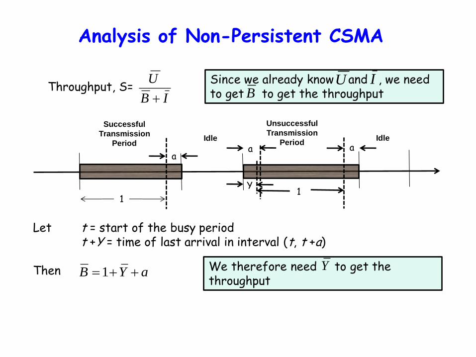
Throughput, S= IB
U
Since we already know and , we need to get to get the throughput B
IU
Successful
Transmission
Period Idle Idle
a
Unsuccessful
Transmission
Period
a
1
a
Y
Let t = start of the busy period t +Y = time of last arrival in interval (t, t +a) Then
1
aYB 1 We therefore need to get the throughput
Y
Analysis of Non-Persistent CSMA
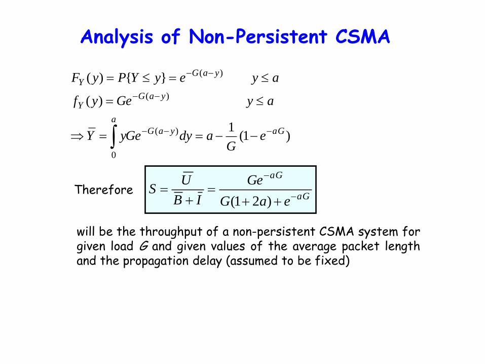
)1(1
)(
}{)(
)(
0
)(
)(
aGyaG
a
yaGY
yaGY
eG
adyGeyY
ayGeyf
ayeyYPyF
Therefore aG
aG
eaG
Ge
IB
US
)21(
will be the throughput of a non-persistent CSMA system for given load G and given values of the average packet length and the propagation delay (assumed to be fixed)
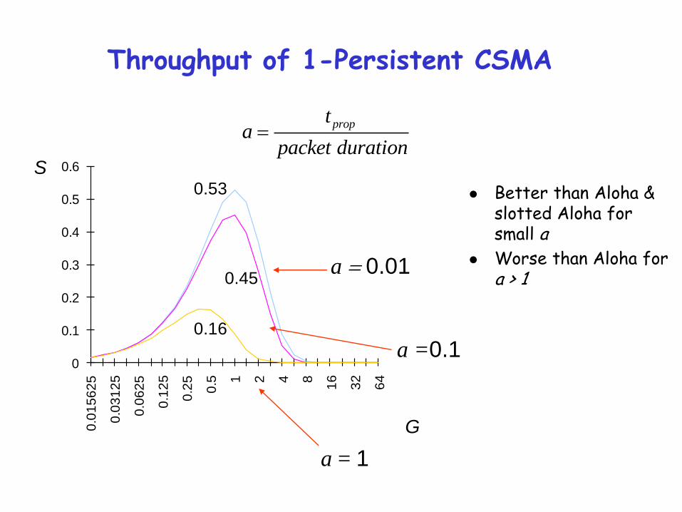
Throughput of 1-Persistent CSMA
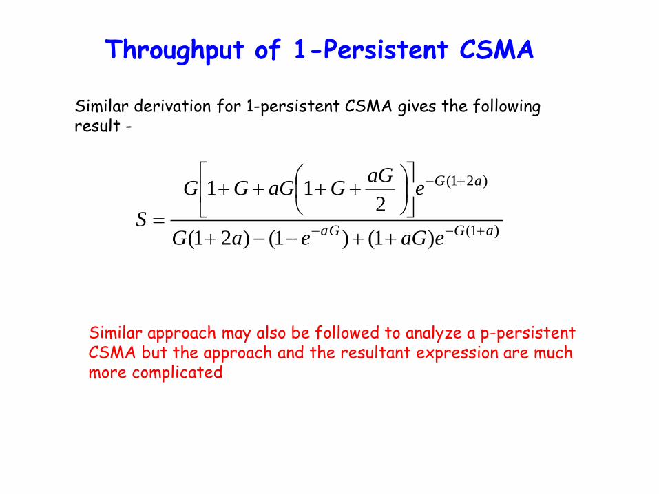
Similar derivation for 1-persistent CSMA gives the following result -
)1(
)21(
)1()1()21(
211
aGaG
aG
eaGeaG
eaG
GaGGG
S
Similar approach may also be followed to analyze a p-persistent CSMA but the approach and the resultant expression are much more complicated
0
0.1
0.2
0.3
0.4
0.5
0.6
0.0
15
62
5
0.0
31
25
0.0
62
5
0.1
25
0.2
5
0.5 1 2 4 8
16
32
64
0.53
0.45
0.16
S
G
a 0.01
a =0.1
a = 1
Throughput of 1-Persistent CSMA
Better than Aloha & slotted Aloha for small a
Worse than Aloha for a > 1
propta
packet duration
0
0.1
0.2
0.3
0.4
0.5
0.6
0.7
0.8
0.9
0.0
1…
0.0
4…
0.1
25
0.3
5…
1
2.8
2…
8
22
.6…
64
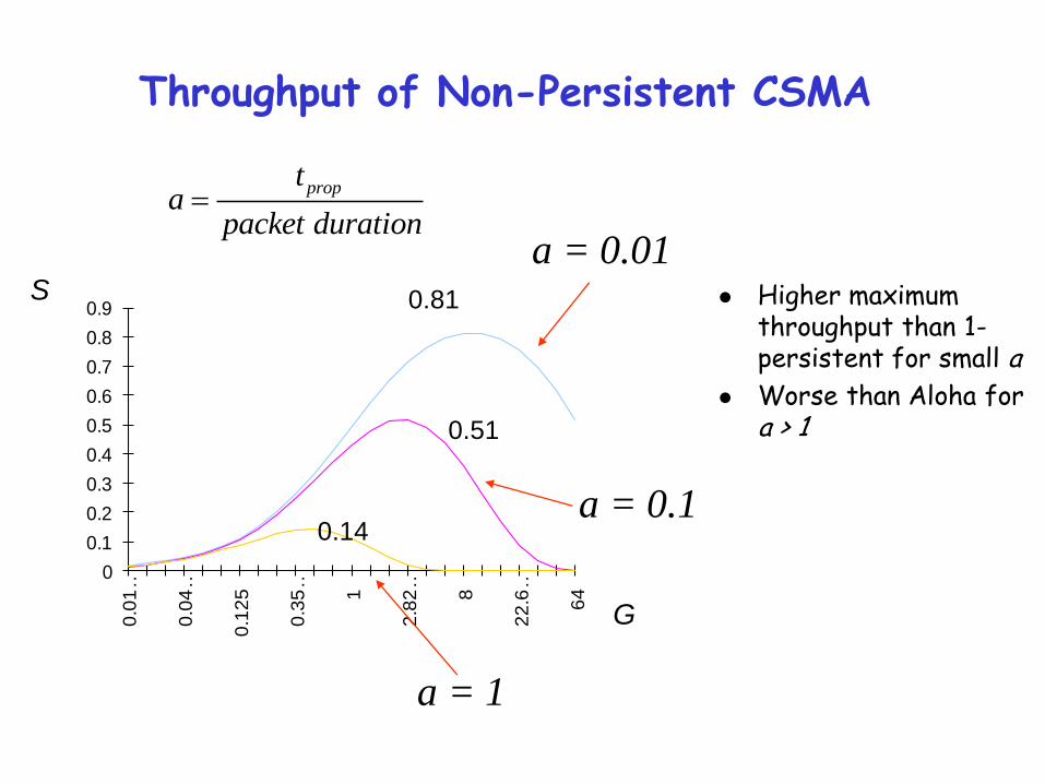
0.81
0.51
0.14
S
G
a = 0.01
Throughput of Non-Persistent CSMA
a = 0.1
a = 1
Higher maximum throughput than 1-persistent for small a
Worse than Aloha for a > 1
propta
packet duration
CSMA with Collision Detection (CSMA/CD)
Monitor for collisions & abort transmission Stations with frames to send, first do carrier sensing
After beginning transmissions, stations continue listening to the medium to detect collisions
If collisions detected, all stations involved stop transmission, reschedule random backoff times, and try again at scheduled times
In CSMA collisions result in wastage of the entire time spent transmitting a complete frame
CSMA-CD reduces this wastage to the time taken to detect a collision and abort the corresponding transmission
Binary Exponential Back off
(used in IEEE 802.3 and Ethernet)
• On detecting a collision, the transmitter aborts and sends a 48-bit jamming signal. It then enters the exponential back off phase where it waits for a random delay before attempting to retransmit.
• The random delay is chosen as K*512 bit times with K random
After the nth collision in a row for the same frame (1n16), choose K randomly from the set {0, 1, ......., 2m-1}, where m=min(n, 10)
Binary Exponential Back off
(used in IEEE 802.3 and Ethernet)
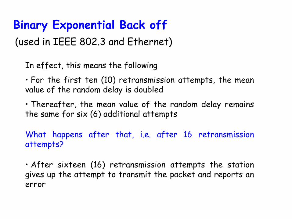
In effect, this means the following
• For the first ten (10) retransmission attempts, the mean value of the random delay is doubled
• Thereafter, the mean value of the random delay remains the same for six (6) additional attempts
What happens after that, i.e. after 16 retransmission attempts?
• After sixteen (16) retransmission attempts the station gives up the attempt to transmit the packet and reports an error

Collision Detection
Collision is detected by changes in the amplitude and pulse width of the signal (from expected values)
Potential problem as signal will attenuate on the line as it travels. If the colliding stations are too far apart, then the collision may not even be detectable
IEEE 802.3 standards avoid this by restricting the maximum length of the coaxial cable and the minimum frame size; minimum frame must be larger than twice the total propagation delay (including repeater delays) between the two farthest nodes of the network (see subsequent slides)
With a star-topology using a Hub, collision detection may be simplified by using logic at the hub. Activity at more than one input at the hub is declared to be a collision and a special collision presence signal is generated and sent out to the stations connected to the hubs
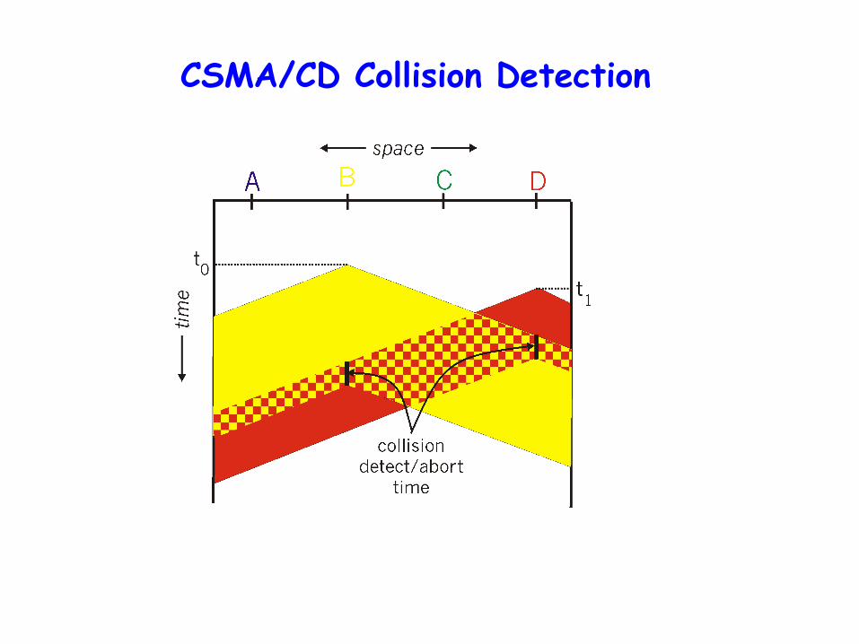
CSMA/CD Collision Detection
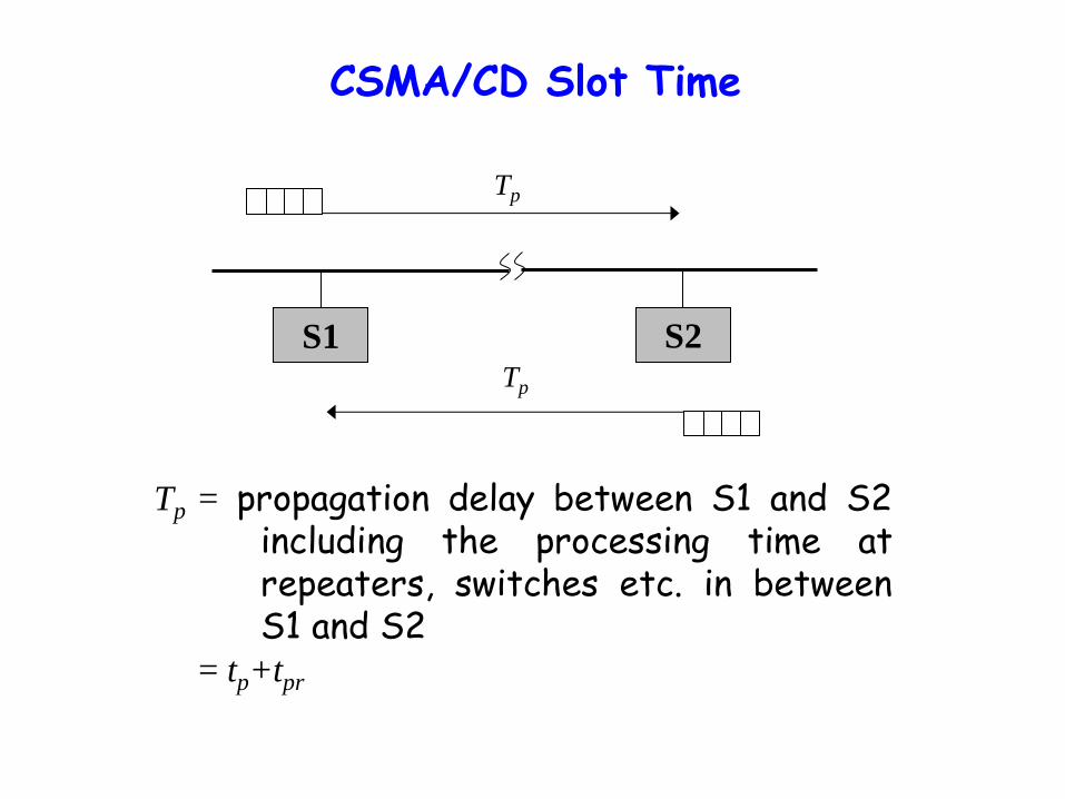
CSMA/CD Slot Time
Tp = propagation delay between S1 and S2 including the processing time at repeaters, switches etc. in between S1 and S2 = tp+tpr
S1 S2
Tp
Tp
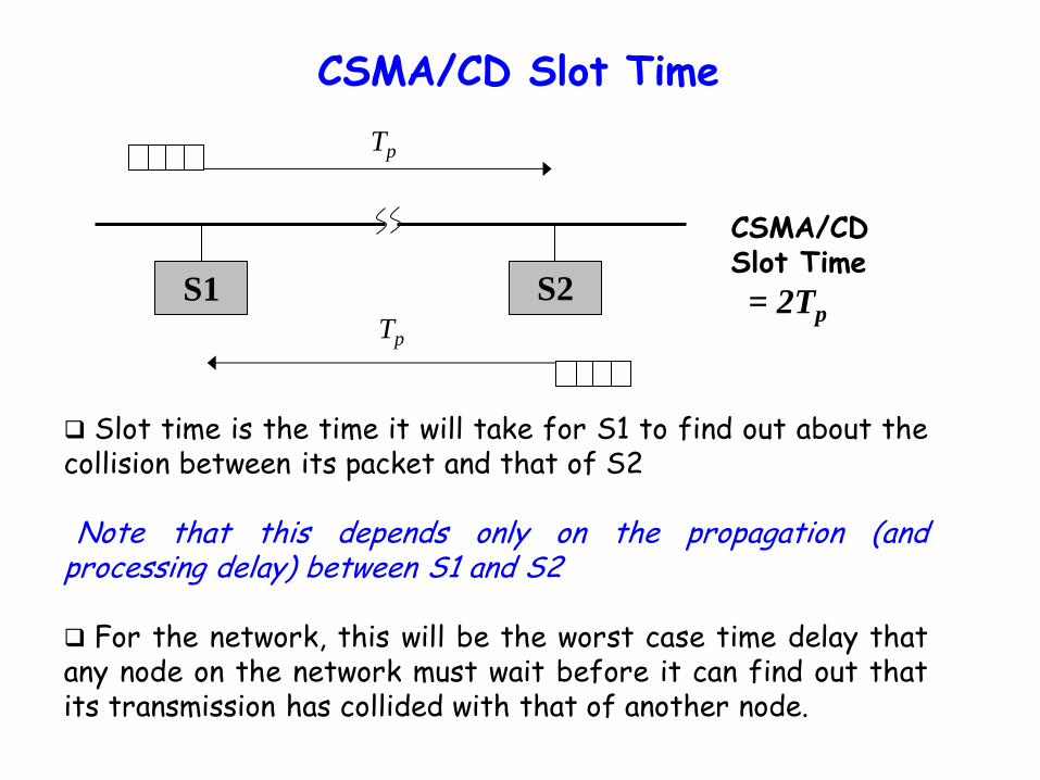
CSMA/CD Slot Time
Slot time is the time it will take for S1 to find out about the collision between its packet and that of S2 Note that this depends only on the propagation (and processing delay) between S1 and S2 For the network, this will be the worst case time delay that any node on the network must wait before it can find out that its transmission has collided with that of another node.
S1 S2
Tp
Tp
CSMA/CD Slot Time
= 2Tp
CSMA/CD Slot Time
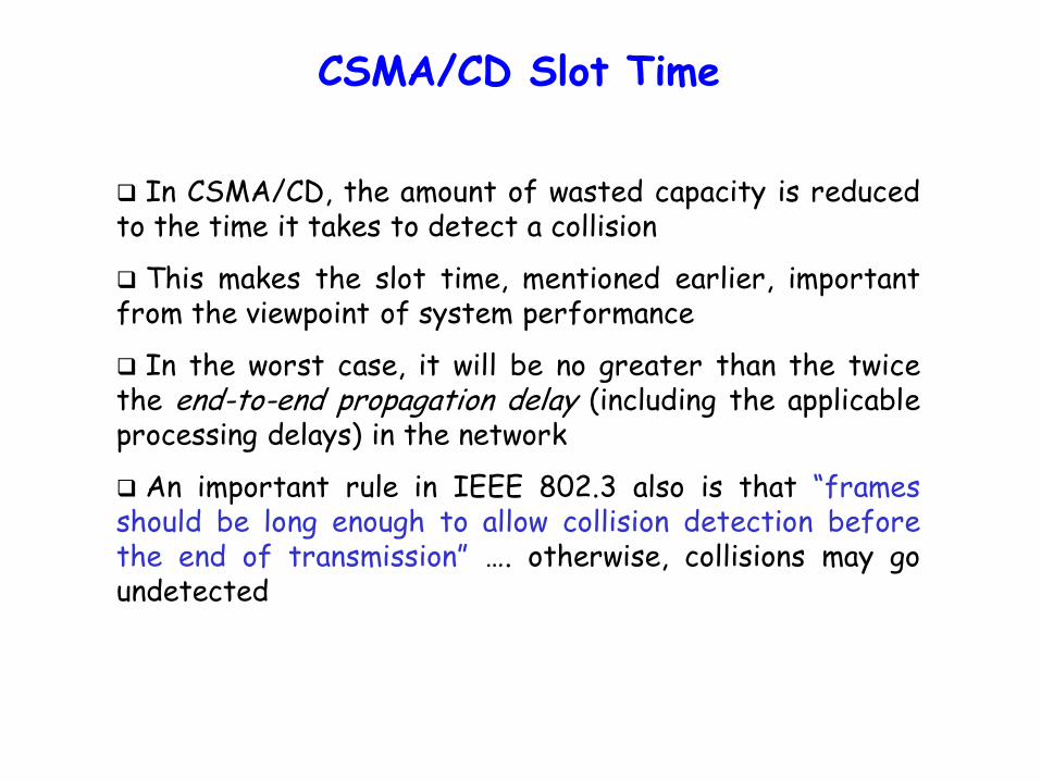
In CSMA/CD, the amount of wasted capacity is reduced to the time it takes to detect a collision
This makes the slot time, mentioned earlier, important from the viewpoint of system performance
In the worst case, it will be no greater than the twice the end-to-end propagation delay (including the applicable processing delays) in the network
An important rule in IEEE 802.3 also is that “frames should be long enough to allow collision detection before the end of transmission” …. otherwise, collisions may go undetected
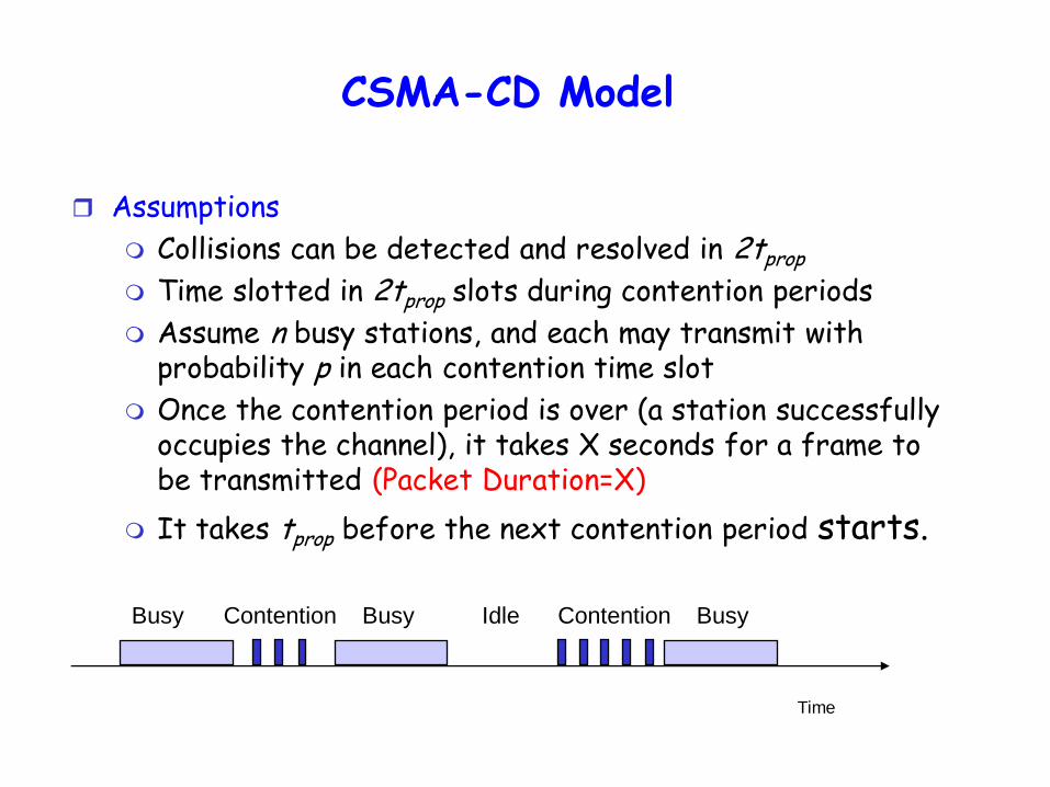
CSMA-CD Model
Assumptions
Collisions can be detected and resolved in 2tprop
Time slotted in 2tprop slots during contention periods
Assume n busy stations, and each may transmit with probability p in each contention time slot
Once the contention period is over (a station successfully occupies the channel), it takes X seconds for a frame to be transmitted (Packet Duration=X)
It takes tprop before the next contention period starts.
Busy Contention Busy
Time
Idle Contention Busy
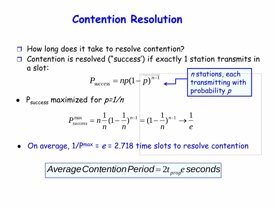
Contention Resolution
How long does it take to resolve contention? Contention is resolved (“success’) if exactly 1 station transmits in
a slot: 1)1( n
success pnpP
Psuccess maximized for p=1/n
ennnnP nn
success
1)
11()
11(
1 11max
On average, 1/Pmax = e = 2.718 time slots to resolve contention
secondsPeriod Contention Average 2 etprop
n stations, each transmitting with probability p
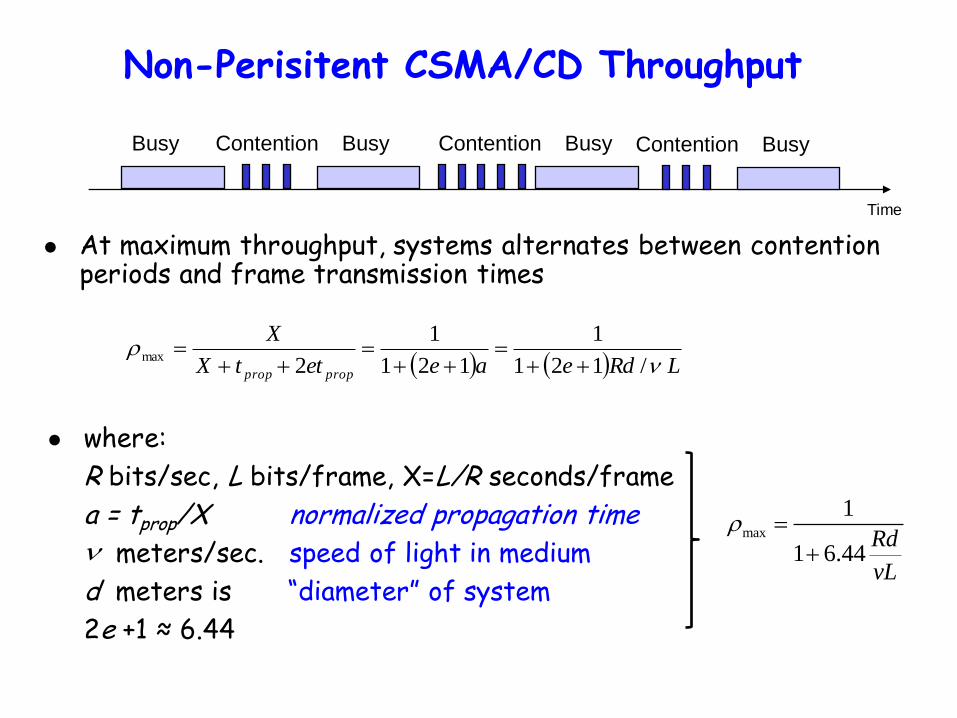
Non-Perisitent CSMA/CD Throughput
At maximum throughput, systems alternates between contention periods and frame transmission times
LRdeaeettX
X
propprop /121
1
121
1
2max
Time
Busy Contention Busy Contention Busy Contention Busy
where:
R bits/sec, L bits/frame, X=L/R seconds/frame
a = tprop/X normalized propagation time
meters/sec. speed of light in medium
d meters is “diameter” of system
2e +1 ≈ 6.44
max
1
1 6.44Rd
vL
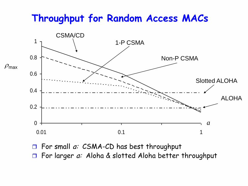
Throughput for Random Access MACs
0
0.2
0.4
0.6
0.8
1
0.01 0.1 1
ALOHA
Slotted ALOHA
1-P CSMA
Non-P CSMA
CSMA/CD
a
max
For small a: CSMA-CD has best throughput For larger a: Aloha & slotted Aloha better throughput

ETHERNET (CSMA-CD Application)
First Ethernet LAN standard used CSMA-CD 1-persistent Carrier Sensing
R = 10 Mbps
tprop = 51.2 microseconds • 512 bits = 64 byte slot
• accommodates 2.5 km + 4 repeaters
Truncated Binary Exponential Backoff • After nth collision, select backoff from {0, 1,…, 2k – 1},
where k=min(n, 10)
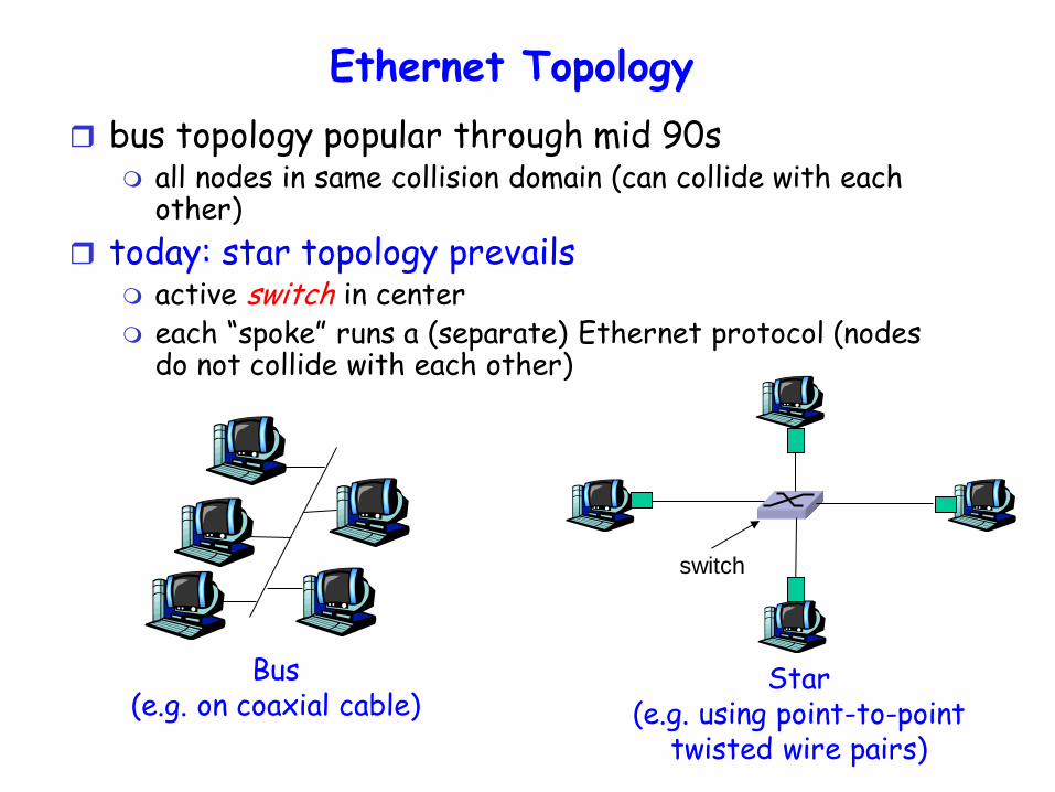
Ethernet Topology
bus topology popular through mid 90s all nodes in same collision domain (can collide with each
other)
today: star topology prevails active switch in center each “spoke” runs a (separate) Ethernet protocol (nodes
do not collide with each other)
switch
Bus (e.g. on coaxial cable)
Star (e.g. using point-to-point
twisted wire pairs)
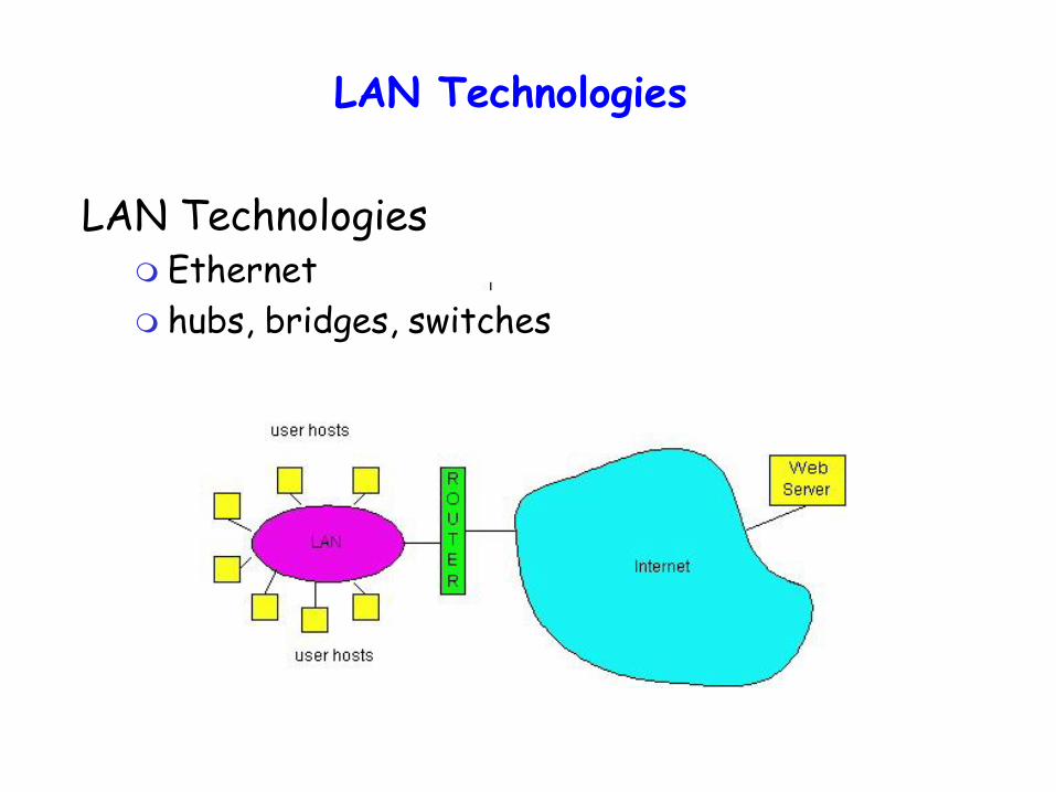
LAN Technologies
LAN Technologies Ethernet
hubs, bridges, switches
MAC Addresses on LANs
LAN (or MAC or physical or Ethernet) address:
used to get datagram from one interface to another physically-connected interface (same network)
48 bit MAC address (for most LANs) burned in the adapter ROM
This is different from the 32-bit IP address which is a
network-layer address
used to get datagram to destination IP network (recall IP network definition)
In effect, the IP Address ensures that the packet is delivered up to the network (LAN) which has the destination station. The MAC address is
then used to deliver the packet to the destination station
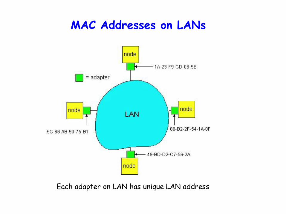
MAC Addresses on LANs
Each adapter on LAN has unique LAN address
MAC Address Features
MAC address allocation administered by IEEE
Manufacturer buys portion of MAC address space (to assure uniqueness)
Analogy:
(a) MAC address: like IC Numbers
(b) IP address: like postal address
MAC flat address => portability can move LAN card from one LAN to another
IP hierarchical address NOT portable depends on IP network to which node is attached
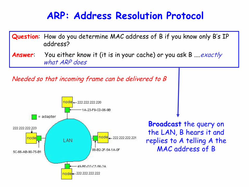
ARP: Address Resolution Protocol
Question: How do you determine MAC address of B if you know only B’s IP address?
Answer: You either know it (it is in your cache) or you ask B ....exactly what ARP does
Broadcast the query on the LAN, B hears it and replies to A telling A the
MAC address of B
Needed so that incoming frame can be delivered to B
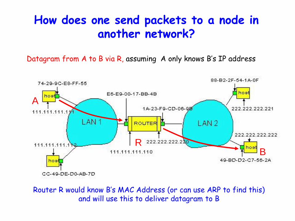
How does one send packets to a node in another network?
Datagram from A to B via R, assuming A only knows B’s IP address
A
R B
Router R would know B’s MAC Address (or can use ARP to find this) and will use this to deliver datagram to B
Ethernet Frame Structure
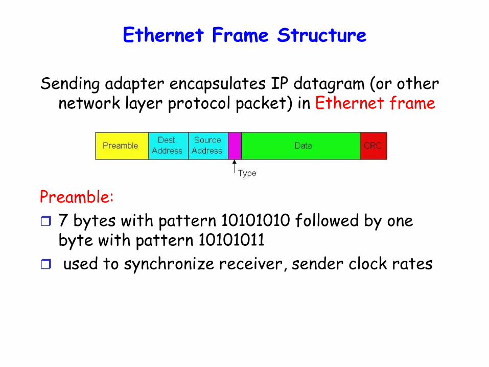
Sending adapter encapsulates IP datagram (or other network layer protocol packet) in Ethernet frame
Preamble:
7 bytes with pattern 10101010 followed by one byte with pattern 10101011
used to synchronize receiver, sender clock rates

Ethernet Frame Structure (more)
Addresses: 6 bytes if adapter receives frame with matching destination
address, or with broadcast address (eg ARP packet), it passes data in frame to net-layer protocol
otherwise, adapter discards frame
Type: indicates the higher layer protocol, mostly IP but others may be supported such as Novell IPX and AppleTalk)
CRC: checked at receiver, if error is detected, the frame is simply dropped
Ethernet: Unreliable, Connectionless operation
Connectionless: No handshaking between sending and receiving adapter
Unreliable: receiving adapter doesn’t send ACKs or NACKs to sending adapter
Ethernet uses CSMA/CD
adapter doesn’t transmit if it senses that some other adapter is transmitting, that is, carrier sense
transmitting adapter aborts when it senses that another adapter is transmitting, that is, collision detection
Before attempting a retransmission, adapter waits a random time following Binary Exponential Backoff (mentioned earlier)

Ethernet CSMA/CD algorithm
1. Adaptor gets datagram from and creates frame
2. If adapter senses channel idle, it starts to transmit frame. If it senses channel busy, waits until channel idle and then transmits
3. If adapter transmits entire frame without detecting another transmission, the adapter is done with frame !
4. If adapter detects another transmission while transmitting, aborts and sends jam signal
Jam Signal: To make sure all other transmitters are aware of collision; length=48 bits
5. After aborting, adapter enters exponential backoff: after the mth collision, adapter chooses a K at random from {0,1,2,…,2m-1}. Adapter waits K*512 bit times and returns to Step 2
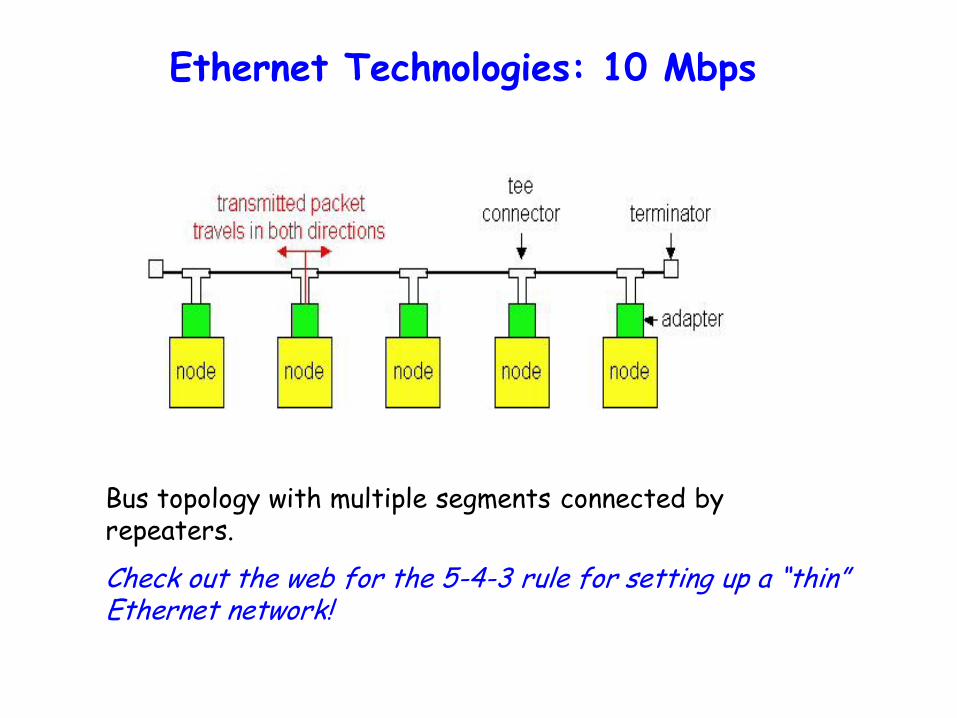
Ethernet Technologies: 10 Mbps
Bus topology with multiple segments connected by repeaters.
Check out the web for the 5-4-3 rule for setting up a “thin” Ethernet network!

Manchester Encoding
Used in 10BaseT, 10Base2
Each bit has a transition
Allows clocks in sending and receiving nodes to synchronize to each other no need for a centralized, global clock among nodes!
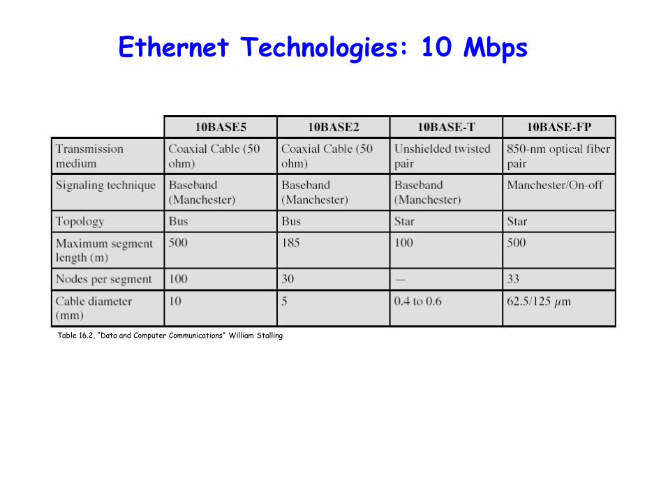
Ethernet Technologies: 10 Mbps
Table 16.2, “Data and Computer Communications” William Stalling
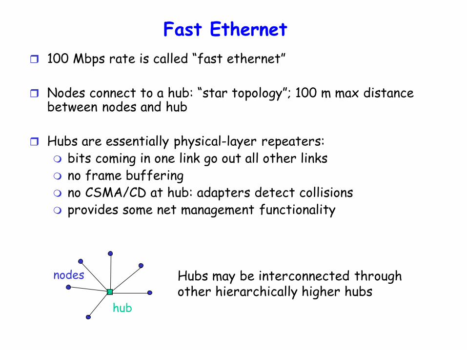
Fast Ethernet
100 Mbps rate is called “fast ethernet”
Nodes connect to a hub: “star topology”; 100 m max distance between nodes and hub
Hubs are essentially physical-layer repeaters: bits coming in one link go out all other links no frame buffering no CSMA/CD at hub: adapters detect collisions provides some net management functionality
hub
nodes Hubs may be interconnected through other hierarchically higher hubs
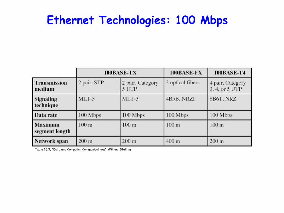
Ethernet Technologies: 100 Mbps
Table 16.3, “Data and Computer Communications” William Stalling
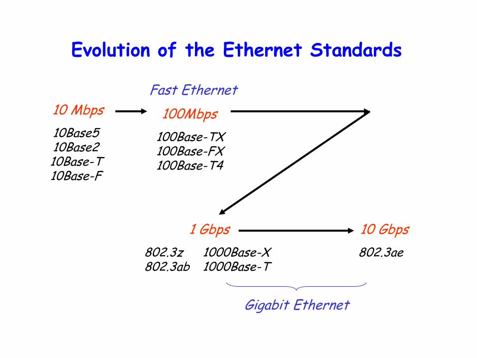
Evolution of the Ethernet Standards
10 Mbps
10Base5 10Base2 10Base-T 10Base-F
1 Gbps
802.3z 1000Base-X 802.3ab 1000Base-T
100Mbps
100Base-TX 100Base-FX 100Base-T4
Fast Ethernet
10 Gbps
802.3ae
Gigabit Ethernet
The Gigabit Ethernet Approach
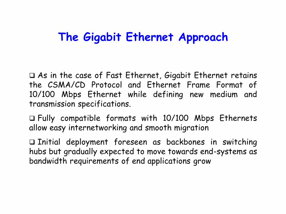
As in the case of Fast Ethernet, Gigabit Ethernet retains the CSMA/CD Protocol and Ethernet Frame Format of 10/100 Mbps Ethernet while defining new medium and transmission specifications.
Fully compatible formats with 10/100 Mbps Ethernets allow easy internetworking and smooth migration
Initial deployment foreseen as backbones in switching hubs but gradually expected to move towards end-systems as bandwidth requirements of end applications grow
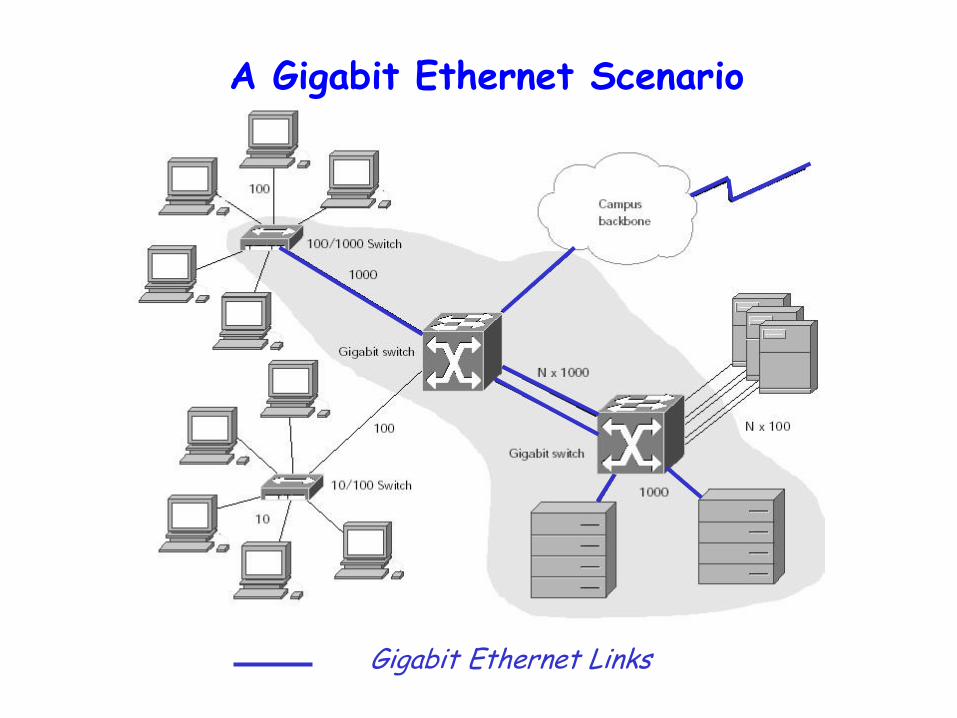
A Gigabit Ethernet Scenario
Gigabit Ethernet Links

Scaling up the speed of CSMA/CD
What is involved if one wants to scale up the speed of a network using Ethernet’s CSMA/CD as the MAC protocol?

Scaling up the speed of CSMA/CD
Ethernet has a minimum frame size of 64 bytes
The reason for enforcing a minimum frame size is to ensure that collision detection can be done even between nodes that are the farthest from each other.
This must be such that it is longer than twice the maximum propagation delay between the two most distant nodes in the network (adding in all the hub and repeater delays in between). This time is also referred to as the slot time of the Ethernet system
Since the minimum frame size is fixed, this effectively limits the maximum propagation (and repeater/hub) delay that may be allowed in an Ethernet network.........and hence limits the cable lengths

Scaling up the speed of CSMA/CD
In the original 10 Mbps Ethernet standards, this was ensured by having -
Minimum Frame Size = 64 bytes
Maximum Cable Length of 2.5 Km with a maximum of four repeaters on any path
Minimum frame size duration is comfortably larger than the slot time for the above!
(Incidentally, it may also be noted that Ethernet also prescribes a maximum frame size as one with 1500 bytes of data.)
Going from 10 Mbps to 100 Mbps
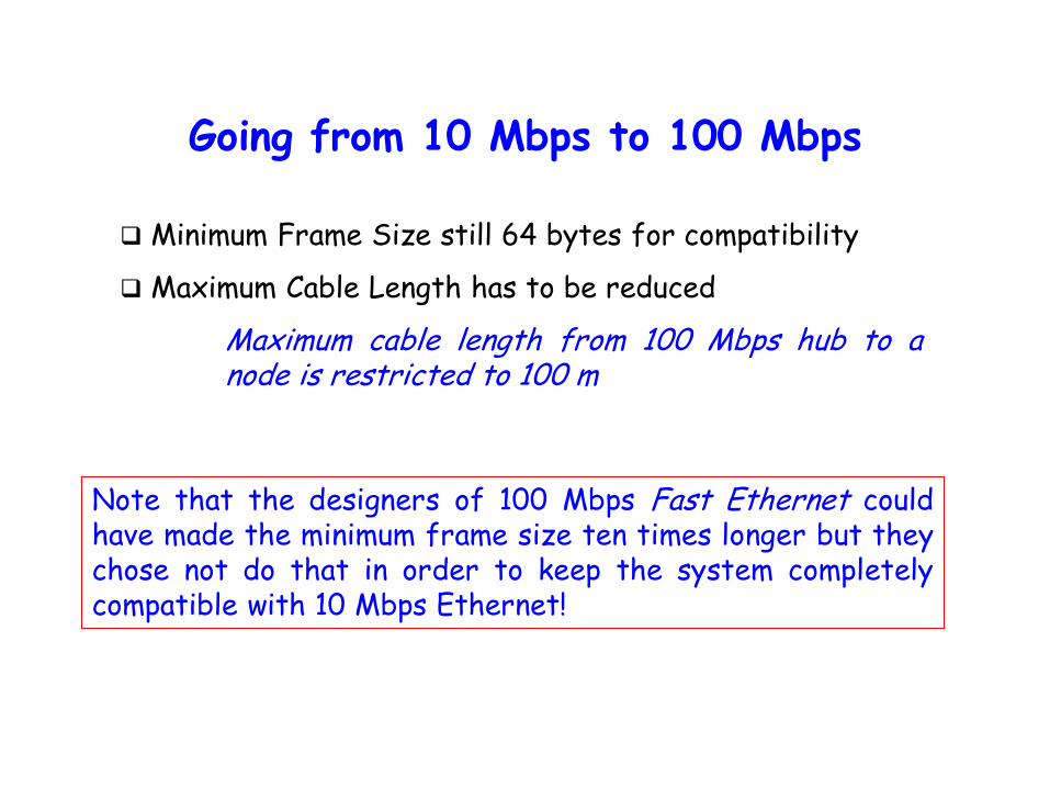
Minimum Frame Size still 64 bytes for compatibility
Maximum Cable Length has to be reduced
Maximum cable length from 100 Mbps hub to a node is restricted to 100 m
Note that the designers of 100 Mbps Fast Ethernet could have made the minimum frame size ten times longer but they chose not do that in order to keep the system completely compatible with 10 Mbps Ethernet!

Going from 100 Mbps to 1 Gbps
Not practical to just reduce the distance to 10 m and keep frame size the same .............. and imagine then what will happen for a speed of 10 Gbps!
In the interests of compatibility, one would not want to change the frame format either, i.e. use longer frames which are incompatible with earlier Ethernet specifications!
..........so what can be done to solve this problem?
Going from 100 Mbps to 1 Gbps
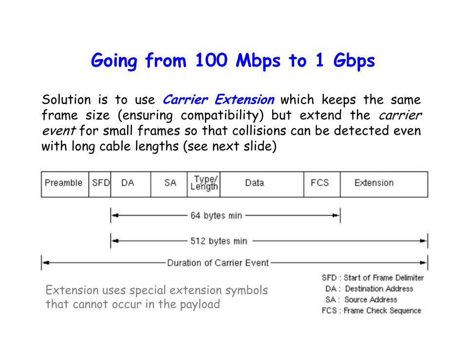
Solution is to use Carrier Extension which keeps the same frame size (ensuring compatibility) but extend the carrier event for small frames so that collisions can be detected even with long cable lengths (see next slide)
Extension uses special extension symbols that cannot occur in the payload

Maximum Hub to Node Distance for 1 Gbps Ethernet
LA
N
MAN/WAN
Going from 100 Mbps to 1 Gbps
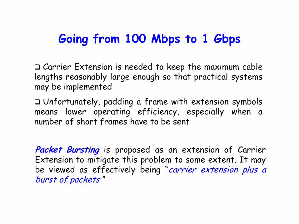
Carrier Extension is needed to keep the maximum cable lengths reasonably large enough so that practical systems may be implemented
Unfortunately, padding a frame with extension symbols means lower operating efficiency, especially when a number of short frames have to be sent
Packet Bursting is proposed as an extension of Carrier Extension to mitigate this problem to some extent. It may be viewed as effectively being “carrier extension plus a burst of packets ”
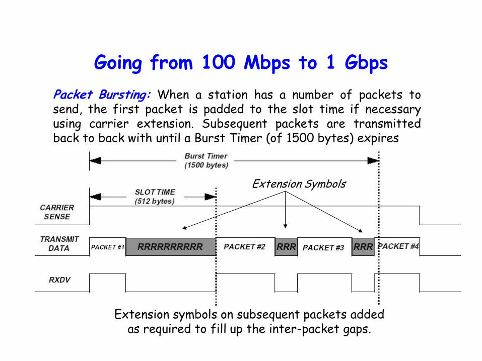
Extension Symbols
Extension symbols on subsequent packets added as required to fill up the inter-packet gaps.
Going from 100 Mbps to 1 Gbps
Packet Bursting: When a station has a number of packets to send, the first packet is padded to the slot time if necessary using carrier extension. Subsequent packets are transmitted back to back with until a Burst Timer (of 1500 bytes) expires
10 Gbps Ethernet
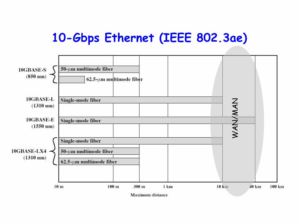
10-Gbps Ethernet (IEEE 802.3ae)
WA
N/M
AN
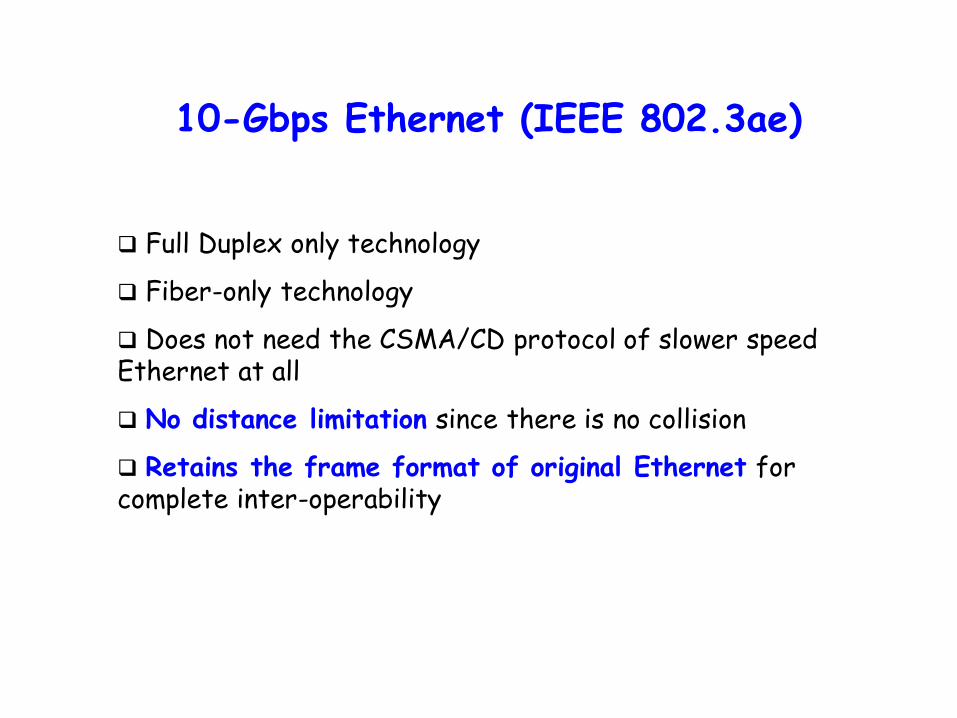
10-Gbps Ethernet (IEEE 802.3ae)
Full Duplex only technology
Fiber-only technology
Does not need the CSMA/CD protocol of slower speed Ethernet at all
No distance limitation since there is no collision
Retains the frame format of original Ethernet for complete inter-operability
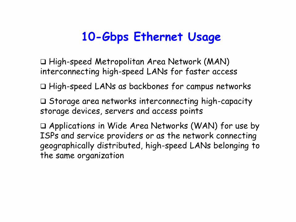
10-Gbps Ethernet Usage
High-speed Metropolitan Area Network (MAN) interconnecting high-speed LANs for faster access
High-speed LANs as backbones for campus networks
Storage area networks interconnecting high-capacity storage devices, servers and access points
Applications in Wide Area Networks (WAN) for use by ISPs and service providers or as the network connecting geographically distributed, high-speed LANs belonging to the same organization
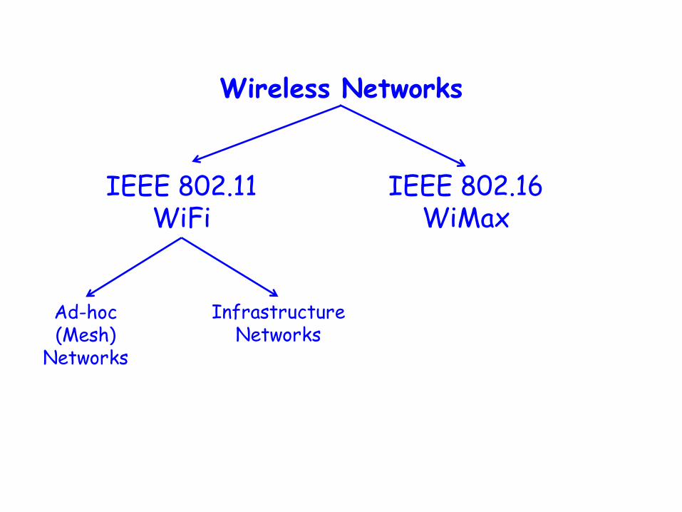
Wireless Networks
IEEE 802.11 WiFi
IEEE 802.16 WiMax
Ad-hoc (Mesh)
Networks
Infrastructure Networks

B D
C A
Ad Hoc Communications
Temporary association of group of stations
Within range of each other Need to exchange information Examples: Presentation in meeting, distributed computer game, war
or disaster scenarios
Nodes not only act as source and destination nodes but also function as intermediate nodes (routers) for others
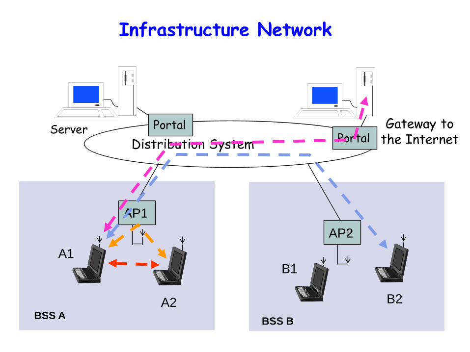
A2 B2
B1
A1
AP1
AP2
Distribution System Server
Gateway to the Internet Portal
Portal
BSS A BSS B
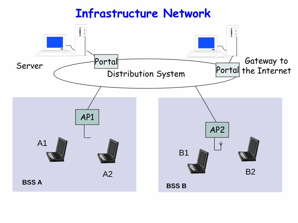
Infrastructure Network

A transmits data frame
(a)
Data Frame Data Frame
A
B C
C transmits data frame & collides with A at B
(b)
C senses medium, station A is hidden from C
Data Frame
B
C A
Hidden Terminal Problem in WiFi
WiFi Networks need new MAC: CSMA-CA (CSMA with Collision Avoidance)
Collision Detection will not work in a wireless network

RTS
A requests to send
B
C
(a)
CTS CTS
A
B
C
B announces A ok to send
(b)
Data Frame
A sends
B
C remains quiet
(c)
CSMA-CA, CSMA with Collision Avoidance
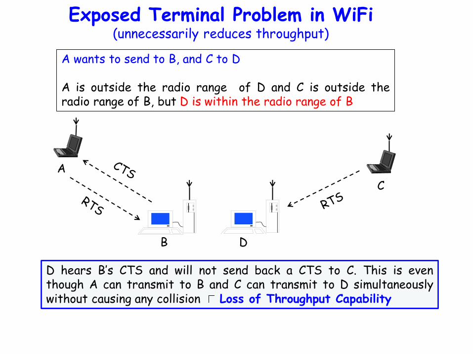
Exposed Terminal Problem in WiFi (unnecessarily reduces throughput)
A wants to send to B, and C to D A is outside the radio range of D and C is outside the radio range of B, but D is within the radio range of B
A
B
C
D
D hears B’s CTS and will not send back a CTS to C. This is even though A can transmit to B and C can transmit to D simultaneously without causing any collision Loss of Throughput Capability
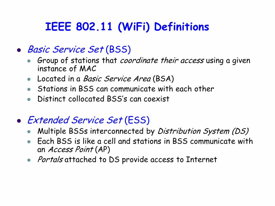
IEEE 802.11 (WiFi) Definitions
Basic Service Set (BSS) Group of stations that coordinate their access using a given
instance of MAC Located in a Basic Service Area (BSA) Stations in BSS can communicate with each other Distinct collocated BSS’s can coexist
Extended Service Set (ESS) Multiple BSSs interconnected by Distribution System (DS) Each BSS is like a cell and stations in BSS communicate with
an Access Point (AP) Portals attached to DS provide access to Internet
A2 B2
B1 A1
AP1
AP2
Distribution System Server Gateway to
the Internet Portal Portal
BSS A BSS B
Infrastructure Network
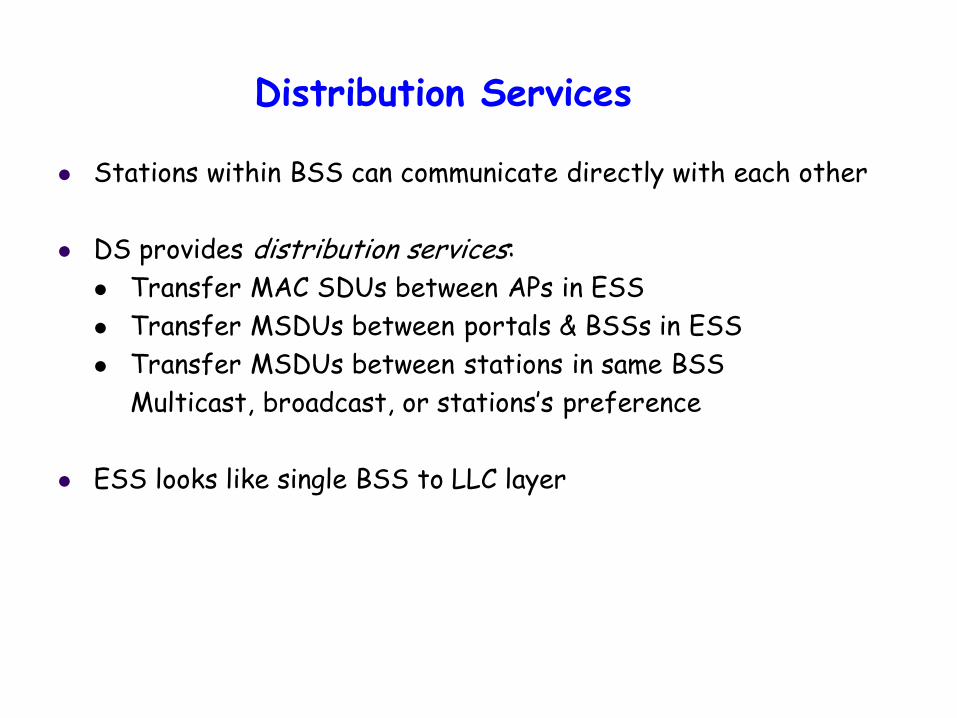
Distribution Services
Stations within BSS can communicate directly with each other
DS provides distribution services:
Transfer MAC SDUs between APs in ESS
Transfer MSDUs between portals & BSSs in ESS
Transfer MSDUs between stations in same BSS
Multicast, broadcast, or stations’s preference
ESS looks like single BSS to LLC layer
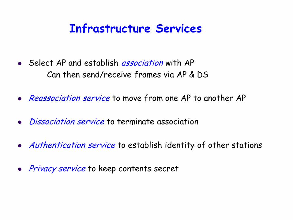
Infrastructure Services
Select AP and establish association with AP
Can then send/receive frames via AP & DS
Reassociation service to move from one AP to another AP
Dissociation service to terminate association
Authentication service to establish identity of other stations
Privacy service to keep contents secret

IEEE 802.11 MAC
MAC sublayer responsibilities
Channel access
PDU addressing, formatting, error checking
Fragmentation & reassembly of MAC SDUs
MAC security service options
Authentication & privacy
MAC management services
Roaming within ESS
Power management
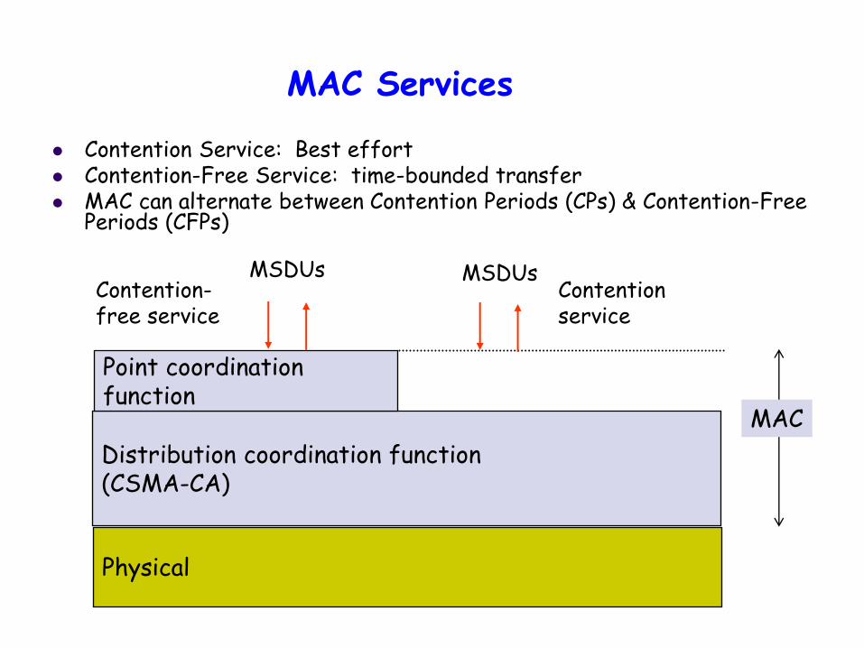
MAC Services
Contention Service: Best effort Contention-Free Service: time-bounded transfer MAC can alternate between Contention Periods (CPs) & Contention-Free
Periods (CFPs)
Physical
Distribution coordination function (CSMA-CA)
Point coordination function
Contention-free service
Contention service
MAC
MSDUs MSDUs

Distributed Coordination Function (DCF)
DCF provides basic access service
Asynchronous best-effort data transfer
All stations contend for access to medium
CSMA-CA
Ready stations wait for completion of transmission
All stations must wait Interframe Space (IFS)
DIFS
DIFS
PIFS
SIFS
Contention window
Next frame
Defer access Wait for reattempt time
Time
Busy medium
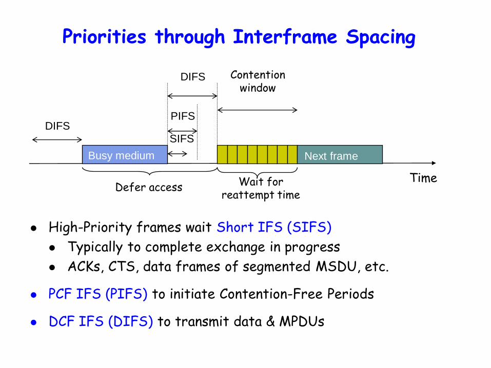
Priorities through Interframe Spacing
High-Priority frames wait Short IFS (SIFS)
Typically to complete exchange in progress
ACKs, CTS, data frames of segmented MSDU, etc.
PCF IFS (PIFS) to initiate Contention-Free Periods
DCF IFS (DIFS) to transmit data & MPDUs
DIFS
DIFS
PIFS
SIFS
Contention window
Next frame
Defer access Wait for reattempt time
Time
Busy medium
Contention & Backoff Behavior
If channel is still idle after DIFS period, ready station can transmit an initial MPDU
If channel becomes busy before DIFS, then station must schedule backoff time for reattempt
Backoff period is integer # of idle contention time slots
Waiting station monitors medium & decrements backoff timer each time an idle contention slot transpires
Station can contend when backoff timer expires
A station that completes a frame transmission is not allowed to transmit immediately
Must first perform a backoff procedure

RTS
CTS CTS
Data Frame
A requests to send
B
C
A
A sends
B
B
C
C remains quiet
B announces A ok to send
(a)
(b)
(c)
ACK B (d)
ACK
B sends ACK

Carrier Sensing in 802.11
Physical Carrier Sensing Analyze all detected frames Monitor relative signal strength from other sources
Virtual Carrier Sensing at MAC sublayer
Source stations informs other stations of transmission time (in msec) for an MPDU
Carried in Duration field of RTS & CTS Stations adjust Network Allocation Vector to indicate when
channel will become idle
Channel busy if either sensing is busy
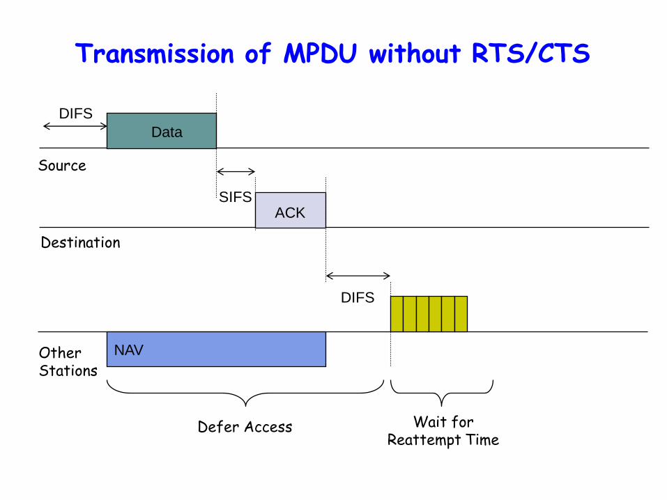
Data
DIFS
SIFS
Defer Access Wait for Reattempt Time
ACK
DIFS
NAV
Source
Destination
Other Stations
Transmission of MPDU without RTS/CTS
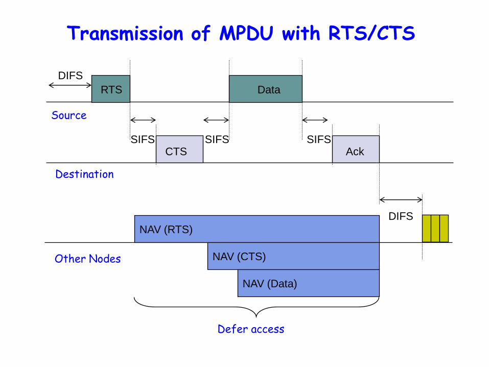
Data
SIFS
Defer access
Ack
DIFS
NAV (RTS)
Source
Destination
Other Nodes
RTS
DIFS
SIFS CTS
SIFS
NAV (CTS)
NAV (Data)
Transmission of MPDU with RTS/CTS
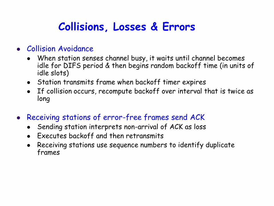
Collisions, Losses & Errors
Collision Avoidance When station senses channel busy, it waits until channel becomes
idle for DIFS period & then begins random backoff time (in units of idle slots)
Station transmits frame when backoff timer expires If collision occurs, recompute backoff over interval that is twice as
long
Receiving stations of error-free frames send ACK Sending station interprets non-arrival of ACK as loss Executes backoff and then retransmits Receiving stations use sequence numbers to identify duplicate
frames
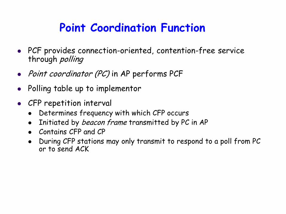
Point Coordination Function
PCF provides connection-oriented, contention-free service through polling
Point coordinator (PC) in AP performs PCF
Polling table up to implementor
CFP repetition interval Determines frequency with which CFP occurs Initiated by beacon frame transmitted by PC in AP Contains CFP and CP During CFP stations may only transmit to respond to a poll from PC
or to send ACK

CF
End
NAV
PIFS
B D1 +
Poll
SIFS
U 1 +
ACK
D2+Ack+
Poll
SIFS SIFS
U 2 +
ACK
SIFS SIFS
Contention-free repetition interval
Contention period
CF_Max_duration
Reset NAV
D1, D2 = frame sent by point coordinator U1, U2 = frame sent by polled station TBTT = target beacon transmission time B = beacon frame
TBTT
PCF Frame Transfer

IEEE 802.11 MAC Layer
MAC Layer Acknowledgement for the transmitted fragment (Multicast packets are not acknowledged in this way)
If the fragment being acknowledged did not suffer from a collision, then its ACK will also not have to undergo a collision. This is ensured by the NAV values of the RTS and CTS frames and by the fact that the DIFS interval is longer than the SIFS interval Each fragment of a multi-fragment packet PDU is separately acknowledged
IEEE 802.11 Fragmentation & Reassembly
LAN protocols, like Ethernet, use large packets (LANPDUs), e.g. Ethernet packets may have upto 1518 bytes of data In a Wireless LAN, smaller packet sizes may be preferred (higher probability of packet error with large packets, smaller packets incur smaller overheads due to packet loss) Fragmentation may therefore happen earlier in an IEEE 802.11 LAN than in an IEEE 802.3 LAN

IEEE 802.11 Fragmentation & Reassembly
802.11 MAC receives a MAC Service Data Unit (MSDU) of length up to 2304 bytes from its higher layer and can optionally divide each MSDU into several smaller MAC Protocol Data Units (MPDU). This is the Fragmentation process. (Each MPDU has its own header and CRC.) Fragments are sent to the destination within the same RTS/CTS exchange using a Stop-&-Wait protocol. The destination node does Reassembly of the fragments to get the original MSDU and pass it on to its higher layer.

IC0101, LAN Infrastructure 97
IEEE 802.11 Fragmentation & Reassembly
MSDU
H CRC H CRC
Fragment 1 Fragment 2
ACK
S
I
F
S
S
I
F
S
Timing Between Fragments of a MSDU

IEEE 802.11: Procedure for a Station to Join an Existing Cell (BSS)
To join a cell (after power-up, sleep or entering a new cell), the station needs to get synchronization information from the AP of that cell. This can be done in one of the two following ways -
Passive Scanning: Station waits to receive a Beacon Frame from the AP. This is sent out periodically with the synchronization information
Active Scanning: Station tries to locate a reachable AP by sending a Probe Request Frame and waits for the Probe Response Frame from the AP for synchronization.
Both methods are valid and any one of them may be chosen. The choice is decided by considerations like power consumption and/or performance.
IEEE 802.11: Authentication Process
Once a station locates an AP and decides to join its BSS, it has to go through an Authentication Process to identify itself as a valid user of the Wireless LAN facility and also verify the identity of the AP.
This is done by the station and AP exchanging information with appropriate passwords.

IEEE 802.11: Association Process
This is started after the Authentication Process has been successfully completed
This involves exchange of information about the station and the BSS and their respective capabilities This allows the overall network (i.e. the set of APs) to know about the current location of the station and the AP it is currently associated with. A station can actually transmit/receive data frames only after the Association Process is over

IEEE 802.11: Roaming
This is the process of a station moving from one BSS to another without losing the connection. The transition from one BSS to another is performed between packet transmissions
Temporary disconnection during roaming will have a bad effect on overall performance as it would require retransmissions to be done by the higher layers
IEEE 802.11: Roaming
The 802.11 protocol does not define how roaming is to be done but does define the basic tools required such as active/passive scanning and a re-association process to change a station from the AP of one BSS to another.
IEEE 802.11: Security Issues
Intruders should not be able to get unauthorized access to the resources of the Wireless LAN
The Authentication Process is expected to prevent this from happening Potential eavesdroppers should not be able to capture and interpret the traffic on the Wireless LAN Prevented by 802.11’s WEP algorithm (Wired Equivalent Privacy) which encrypts the transmissions on the wireless medium. WEP is a simple algorithm based on RSA which is reasonably strong.

IC0101, LAN Infrastructure 104
IEEE 802.11: Power Saving Issues
Power saving is important at the mobile stations as battery power is a scarce resource 802.11 standards directly address this issue and provide the mechanism for stations to go into sleep mode without losing data The AP keeps a continually updated record of the stations currently in Power Saving mode. Data intended for these stations is buffered at the AP until either the station sends a polling request for it or it changes its operational mode. Apart from synchronization information, Beacon Frames from the AP also send information about which Power Saving Stations have frames buffered at the AP. The indicated stations can then download their data as per their convenience.
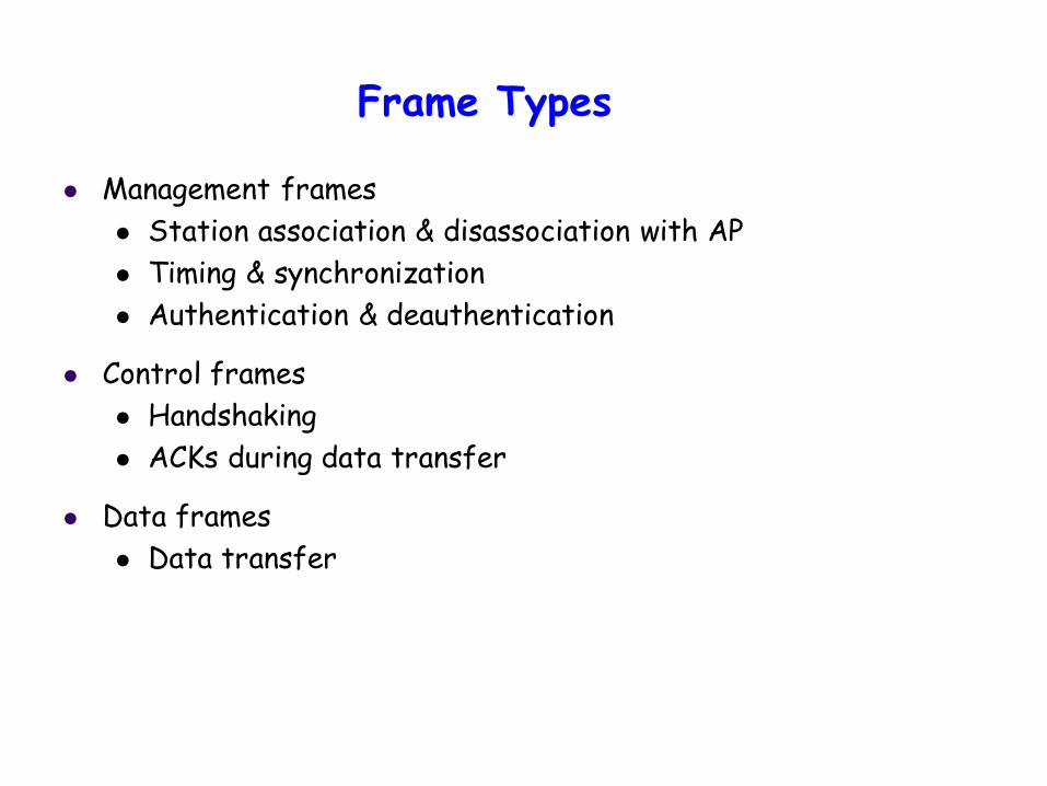
Frame Types
Management frames
Station association & disassociation with AP
Timing & synchronization
Authentication & deauthentication
Control frames
Handshaking
ACKs during data transfer
Data frames
Data transfer
Address
2
Frame
Control
Duration/
ID
Address
1
Address
3
Sequence
control
Address
4
Frame
body CRC
2 2 6 6 6 2 6 0-2312 4
MAC header (bytes)
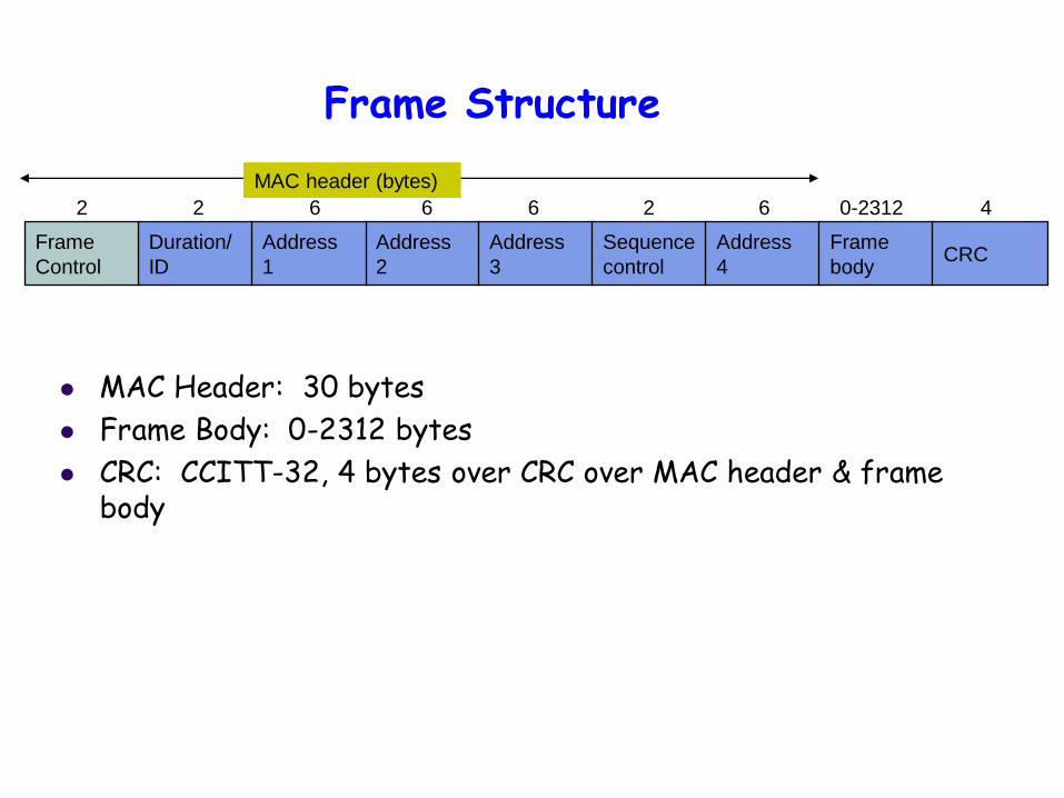
Frame Structure
MAC Header: 30 bytes
Frame Body: 0-2312 bytes
CRC: CCITT-32, 4 bytes over CRC over MAC header & frame body
Address
2
Frame
Control
Duration/
ID
Address
1
Address
3
Sequence
control
Address
4
Frame
body CRC
Protocol
version Type Subtype
To
DS
From
DS
More
frag Retry
Pwr
mgt
More
data WEP Rsvd
2 2 6 6 6 2 6 0-2312 4
2 2
MAC header (bytes)
4 1 1 1 1 1 1 1 1
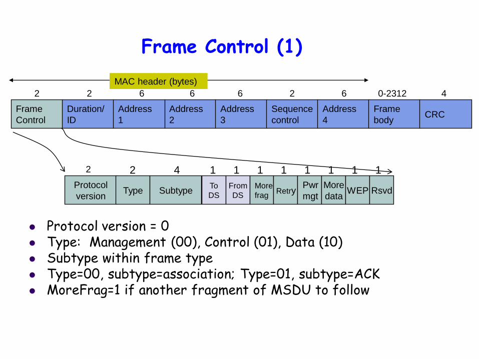
Frame Control (1)
Protocol version = 0 Type: Management (00), Control (01), Data (10) Subtype within frame type Type=00, subtype=association; Type=01, subtype=ACK MoreFrag=1 if another fragment of MSDU to follow
To
DS
From
DS
Address
1
Address
2
Address
3
Address
4
0 0 Destination
address
Source
address BSSID N/A
0 1 Destination
address BSSID
Source
address N/A
1 0 BSSID Source
address
Destination
address N/A
1 1 Receiver
address
Transmitter
address
Destination
address
Source
address
Meaning
Data frame from station to
station within a BSS
Data frame exiting the DS
Data frame destined for the
DS
WDS frame being distributed
from AP to AP
Address
2
Frame
Control
Duration/
ID
Address
1
Address
3
Sequence
control
Address
4
Frame
body CRC
Protocol
version Type Subtype
To
DS
From
DS
More
frag Retry
Pwr
mgt
More
data WEP Rsvd
2 2 6 6 6 2 6 0-2312 4
2 2 4 1 1 1 1 1 1 1 1
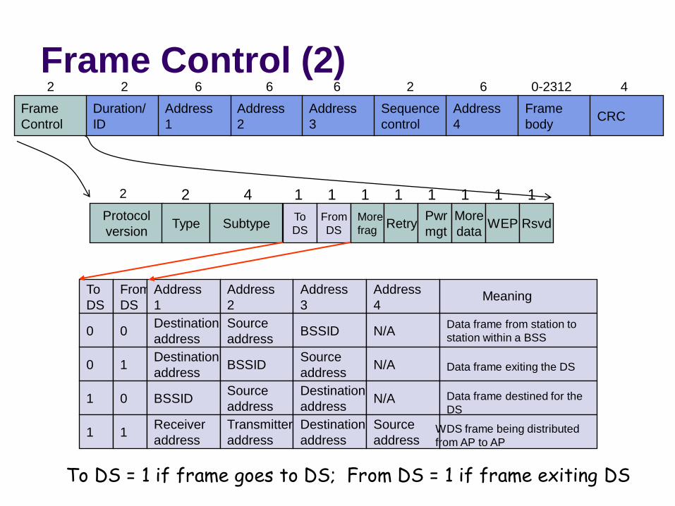
To DS = 1 if frame goes to DS; From DS = 1 if frame exiting DS
Frame Control (2)
Address
2
Frame
Control
Duration/
ID
Address
1
Address
3
Sequence
control
Address
4
Frame
body CRC
Protocol
version Type Subtype
To
DS
From
DS
More
frag Retry
Pwr
mgt
More
data WEP Rsvd
2 2 6 6 6 2 6 0-2312 4
2 2
MAC header (bytes)
4 1 1 1 1 1 1 1 1
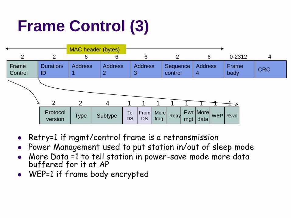
Frame Control (3)
Retry=1 if mgmt/control frame is a retransmission Power Management used to put station in/out of sleep mode More Data =1 to tell station in power-save mode more data
buffered for it at AP WEP=1 if frame body encrypted

Physic
al
layer
LLC
Physical layer
convergence
procedure
Physical medium
dependent
MAC
layer
PLCP
preamble
LLC PDU
MAC SDU MAC
header CRC
PLCP
header PLCP PDU
Physical Layers
802.11 designed to Support LLC Operate over many physical layers
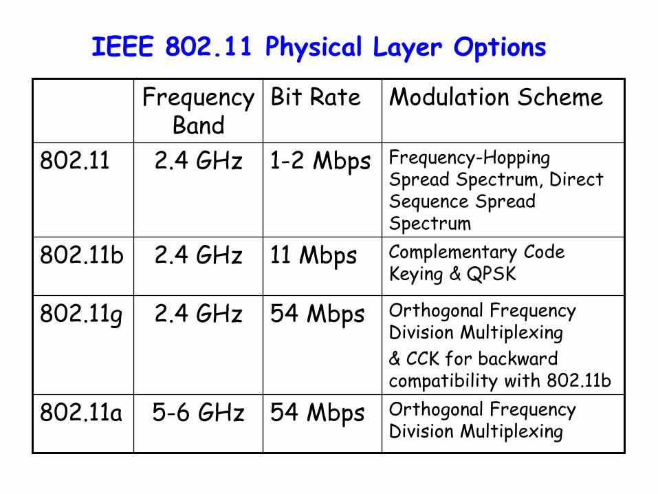
IEEE 802.11 Physical Layer Options
Frequency Band
Bit Rate Modulation Scheme
802.11 2.4 GHz 1-2 Mbps Frequency-Hopping Spread Spectrum, Direct Sequence Spread Spectrum
802.11b 2.4 GHz 11 Mbps Complementary Code Keying & QPSK
802.11g 2.4 GHz 54 Mbps Orthogonal Frequency Division Multiplexing
& CCK for backward compatibility with 802.11b
802.11a 5-6 GHz 54 Mbps Orthogonal Frequency Division Multiplexing
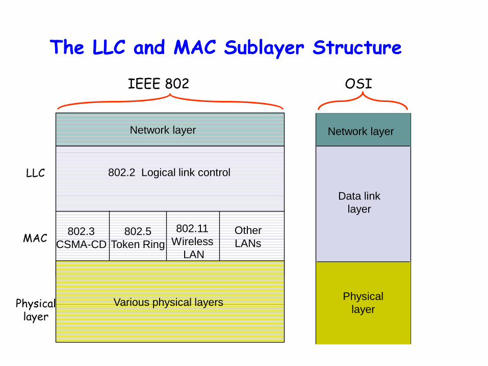
The LLC and MAC Sublayer Structure
Data link
layer
802.3
CSMA-CD
802.5
Token Ring
802.2 Logical link control
Physical layer
MAC
LLC
802.11
Wireless
LAN
Network layer Network layer
Physical
layer
OSI IEEE 802
Various physical layers
Other
LANs
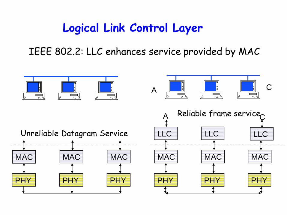
Logical Link Control Layer
PHY
MAC
PHY
MAC
PHY
MAC
Unreliable Datagram Service
PHY
MAC
PHY
MAC
PHY
MAC
Reliable frame service
LLC LLC LLC
A C
A C
IEEE 802.2: LLC enhances service provided by MAC
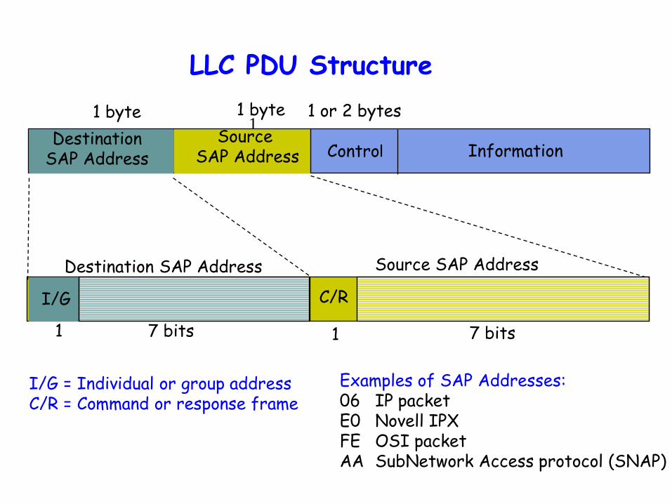
LLC PDU Structure
1 Source
SAP Address Information
1 byte
Control
1 or 2 bytes
Destination SAP Address Source SAP Address
I/G
7 bits 1
C/R
7 bits 1
I/G = Individual or group address C/R = Command or response frame
Destination SAP Address
1 byte
Examples of SAP Addresses: 06 IP packet E0 Novell IPX FE OSI packet AA SubNetwork Access protocol (SNAP)
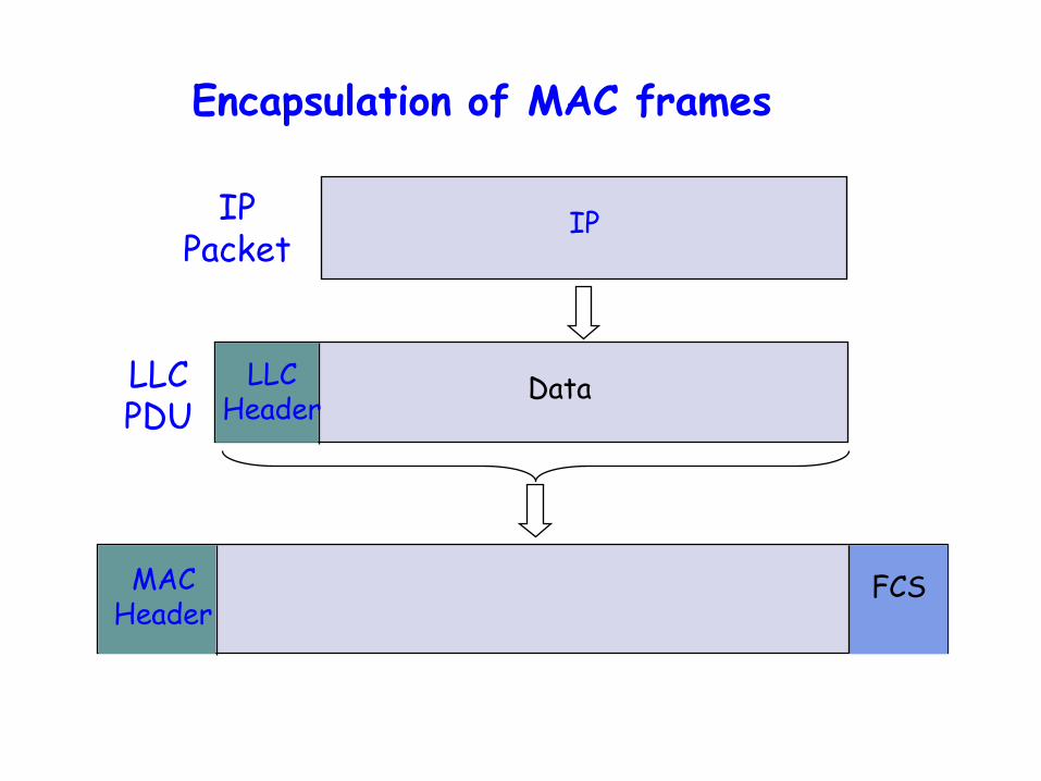
Encapsulation of MAC frames
IP
LLC Header
Data
MAC Header
FCS
LLC PDU
IP Packet
Interconnecting LAN Segments
Hubs
Bridges
Switches Remark: switches are essentially multi-port
bridges.
What we say about bridges also holds for switches!

Interconnecting with Hubs
Backbone hub interconnects LAN segments Extends max distance between nodes But individual segment collision domains become one
large collision domain if a node in CS and a node EE transmit at same time: collision
Can’t interconnect 10BaseT & 100BaseT
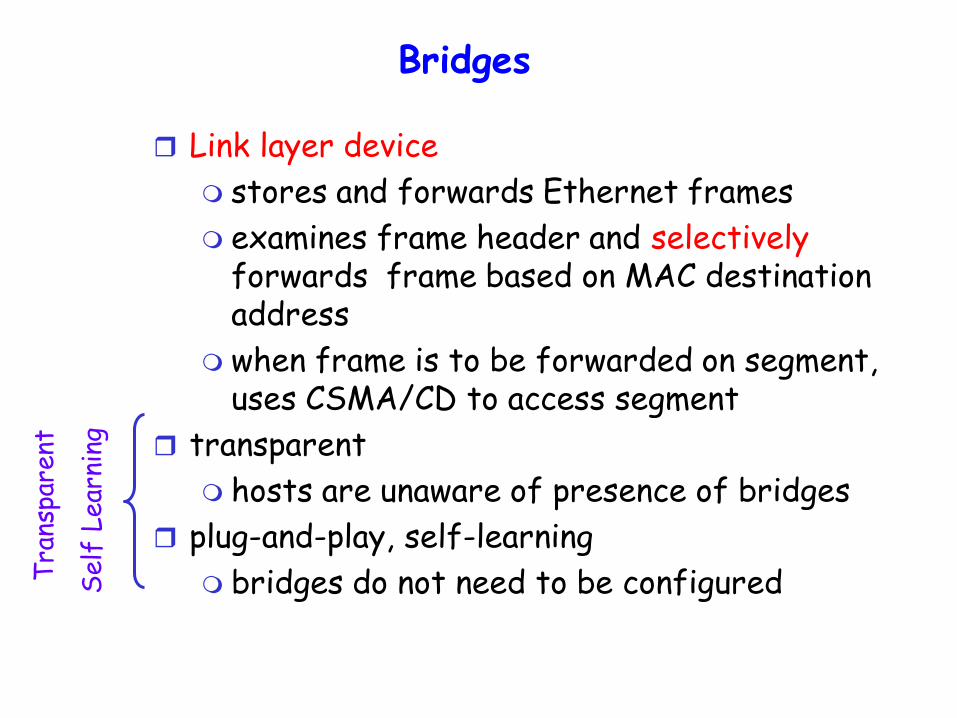
Bridges
Link layer device
stores and forwards Ethernet frames
examines frame header and selectively forwards frame based on MAC destination address
when frame is to be forwarded on segment, uses CSMA/CD to access segment
transparent
hosts are unaware of presence of bridges
plug-and-play, self-learning
bridges do not need to be configured
Tra
nspa
rent
Sel
f Lea
rnin
g
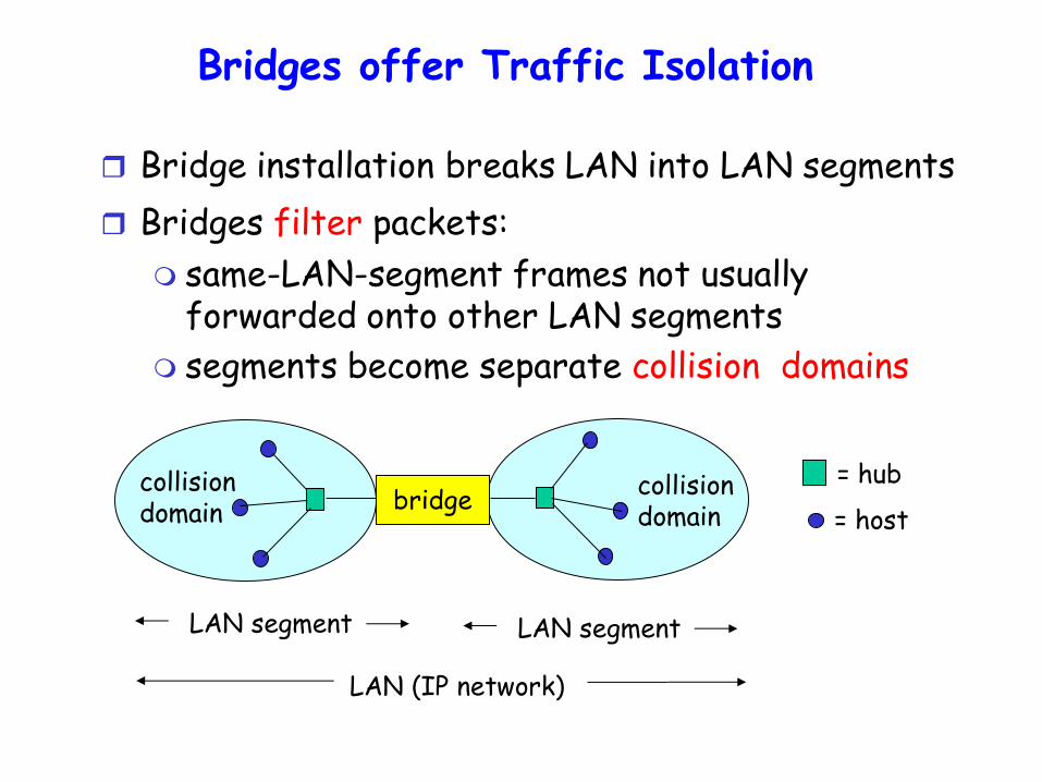
Bridges offer Traffic Isolation
Bridge installation breaks LAN into LAN segments
Bridges filter packets: same-LAN-segment frames not usually
forwarded onto other LAN segments
segments become separate collision domains
bridge collision domain
collision domain
= hub
= host
LAN (IP network)
LAN segment LAN segment
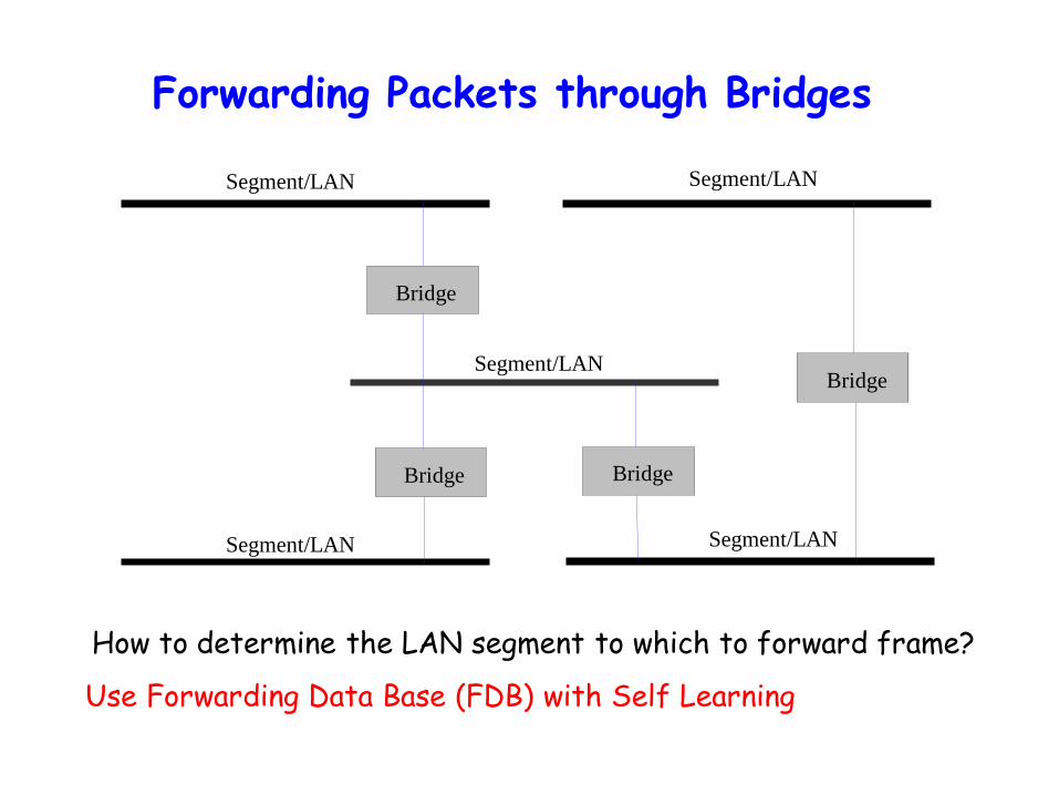
Forwarding Packets through Bridges
How to determine the LAN segment to which to forward frame?
Use Forwarding Data Base (FDB) with Self Learning
Bridge
Bridge
Bridge
Bridge
Segment/LAN
Segment/LAN
Segment/LAN
Segment/LAN
Segment/LAN
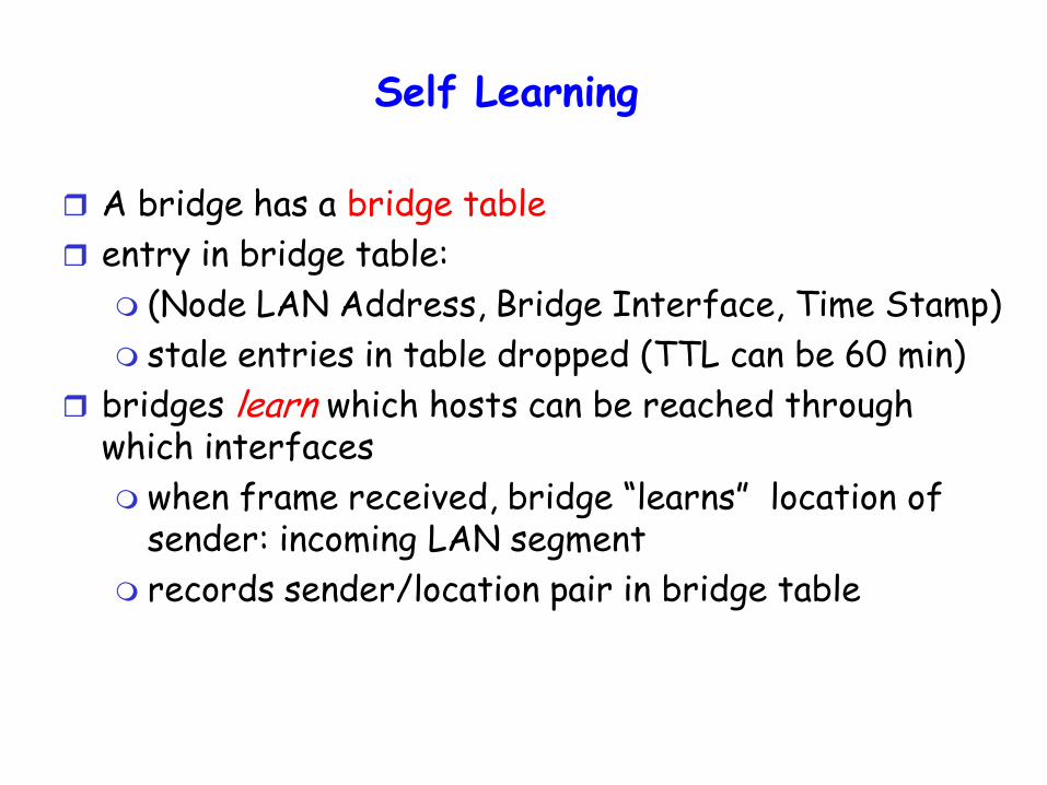
Self Learning
A bridge has a bridge table
entry in bridge table:
(Node LAN Address, Bridge Interface, Time Stamp)
stale entries in table dropped (TTL can be 60 min)
bridges learn which hosts can be reached through which interfaces
when frame received, bridge “learns” location of sender: incoming LAN segment
records sender/location pair in bridge table
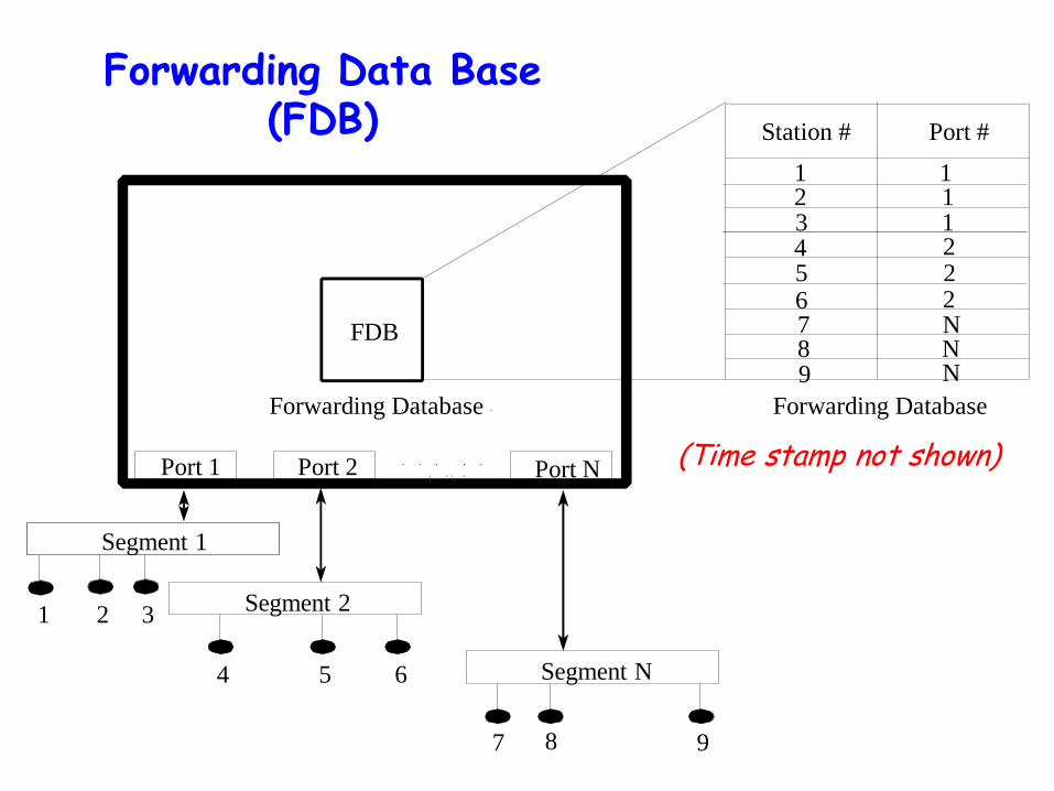
Forwarding Data Base (FDB)
7 8 9
Port 1 Port 2 Port N
Segment 1
Segment 2
Segment N
3
4 5 6
1 2
Forwarding Database
FDB
Station # Port #
1 1 2 1 3 1 4 2 5 2 6 2 7 N 8 N 9 N
Forwarding Database
(Time stamp not shown)
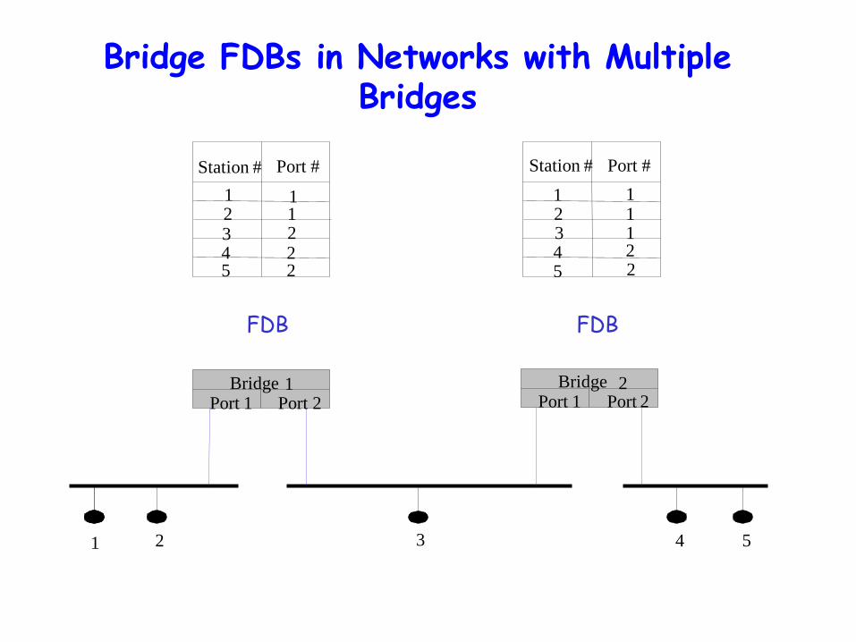
Bridge FDBs in Networks with Multiple Bridges
Bridge Port Port
Bridge Port Port
1 1 1
2 2 2
1 2 3 4 5
Station # Port # Station # Port #
1 2 3 4 5
1 2 3 4 5
1 1 2 2 2
1 1 1 2 2
FDB FDB
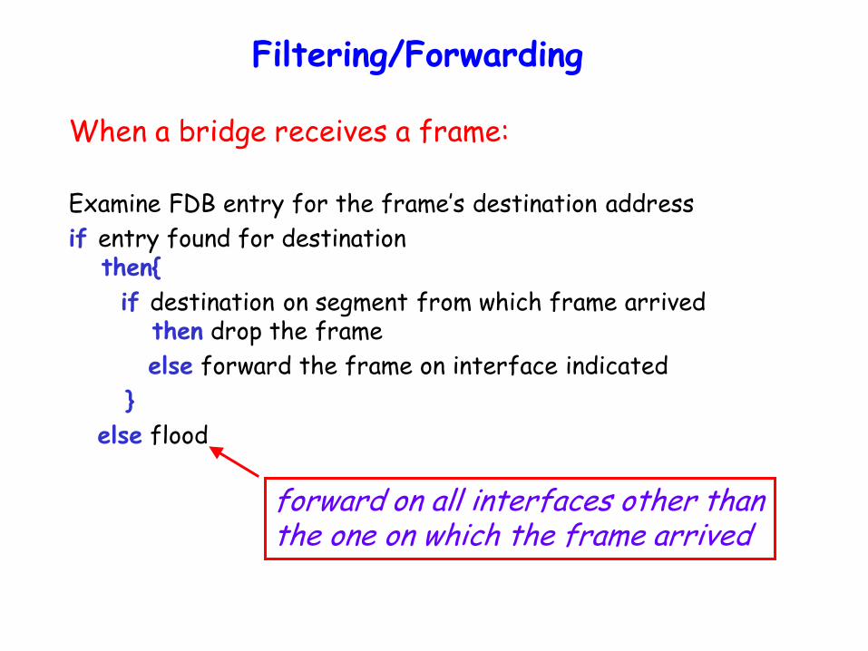
Filtering/Forwarding
When a bridge receives a frame:
Examine FDB entry for the frame’s destination address
if entry found for destination then{
if destination on segment from which frame arrived then drop the frame
else forward the frame on interface indicated
}
else flood
forward on all interfaces other than the one on which the frame arrived
Spanning Tree Algorithm (STA)
A Spanning Tree is a path list of one and only one path between all the nodes in an extended LAN (i.e. multiple LANs connected by bridges)
If the network is represented by a graph, then the spanning tree maintains the connectivity of all the nodes in the graph but removes all possible loops
STA is needed because logical loops can lead to packets circulating endlessly in the network
Following the STA, the network automatically disables certain bridges/ports. Note that these bridges are not removed since they may be needed if the topology changes and the spanning tree is reconfigured dynamically.

Spanning Tree Algorithm (STA)
To implement the STA in a network -
each bridge must have a unique Bridge ID
each port in the bridge must have a unique Port ID
all the bridges on the LAN must recognize a unique MAC group address
B1
P1 P2 P3
B1: Bridge ID
P1, P2, P3: Port IDs Example

Sample Topology and Spanning Tree
B1
P1
P2
Segment 1
Segment
2
Segment
3
Segment 4
B2
P1
P2
B4
P1
P2
B5
P1
P2
B3
P1
P2
P3
A Sample Topology of a Bridged LAN
All LANs assumed to have equal cost
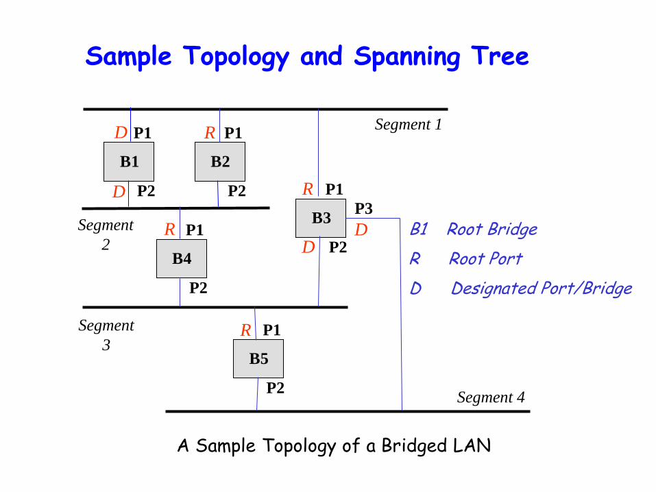
Sample Topology and Spanning Tree
B1
P1
P2
Segment 1
Segment
2
Segment
3
Segment 4
B2
P1
P2
B4
P1
P2
B5
P1
P2
B3
P1
P2
P3
B1 Root Bridge
R Root Port
D Designated Port/Bridge
R
R
R
R D
D
D D
A Sample Topology of a Bridged LAN

Sample Topology and Spanning Tree
B1
P1
P2
Segment 1
Segment
2
Segment
3
Segment 4
B3
P1
P2
P3
R
D
D
D D
Even though bridges B2, B4 and B5 have not been shown, they are still present and may be used if the topology changes or if bridges or links fail.
A Sample Topology of a Bridged LAN
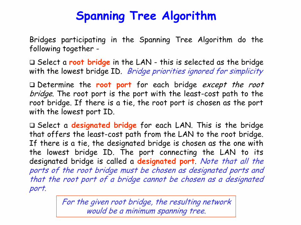
Spanning Tree Algorithm
Bridges participating in the Spanning Tree Algorithm do the following together -
Select a root bridge in the LAN - this is selected as the bridge with the lowest bridge ID. Bridge priorities ignored for simplicity
Determine the root port for each bridge except the root bridge. The root port is the port with the least-cost path to the root bridge. If there is a tie, the root port is chosen as the port with the lowest port ID.
Select a designated bridge for each LAN. This is the bridge that offers the least-cost path from the LAN to the root bridge. If there is a tie, the designated bridge is chosen as the one with the lowest bridge ID. The port connecting the LAN to its designated bridge is called a designated port. Note that all the ports of the root bridge must be chosen as designated ports and that the root port of a bridge cannot be chosen as a designated port.
For the given root bridge, the resulting network would be a minimum spanning tree.
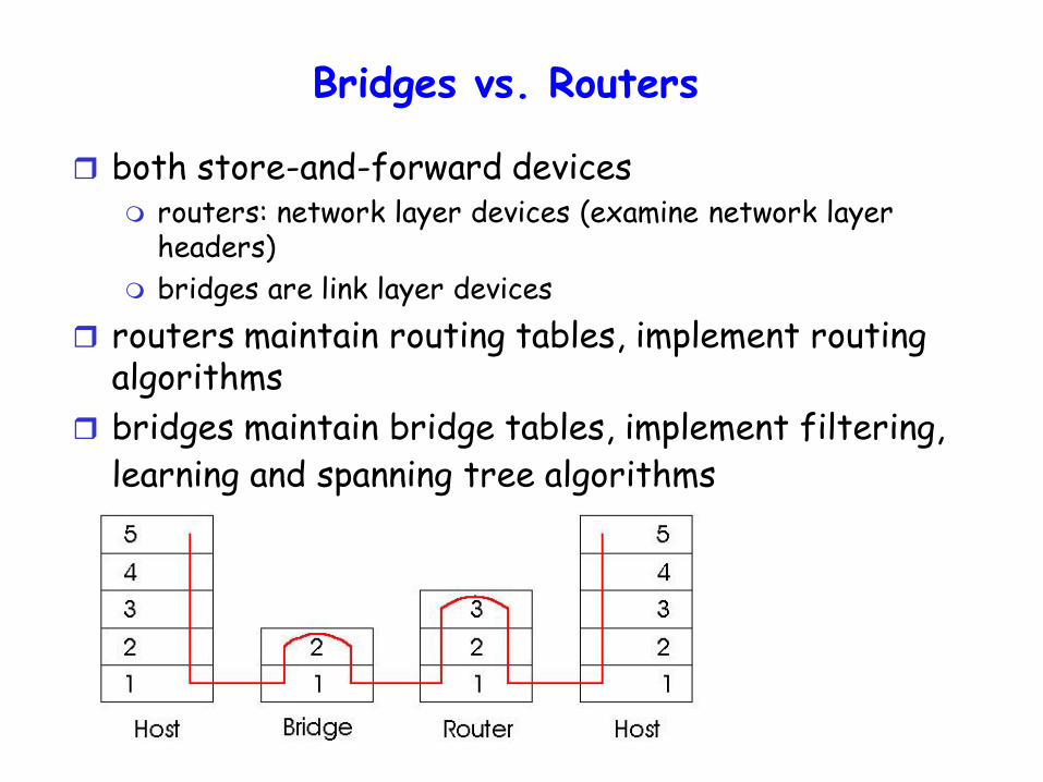
Bridges vs. Routers
both store-and-forward devices routers: network layer devices (examine network layer
headers)
bridges are link layer devices
routers maintain routing tables, implement routing algorithms
bridges maintain bridge tables, implement filtering, learning and spanning tree algorithms
Routers vs. Bridges
Bridges + and -
+ Bridge operation is simpler requiring less packet processing
+ Bridge tables are self learning
- All traffic confined to spanning tree, even when alternative bandwidth is available
- Bridges do not offer protection from broadcast storms
Routers vs. Bridges
Routers + and -
+ arbitrary topologies can be supported, cycling is limited by TTL counters (and good routing protocols)
+ provide protection against broadcast storms
- require IP address configuration (not plug and play)
- require higher packet processing
bridges do well in small (few hundred hosts) while routers used in large networks (thousands of hosts)
Ethernet Switches
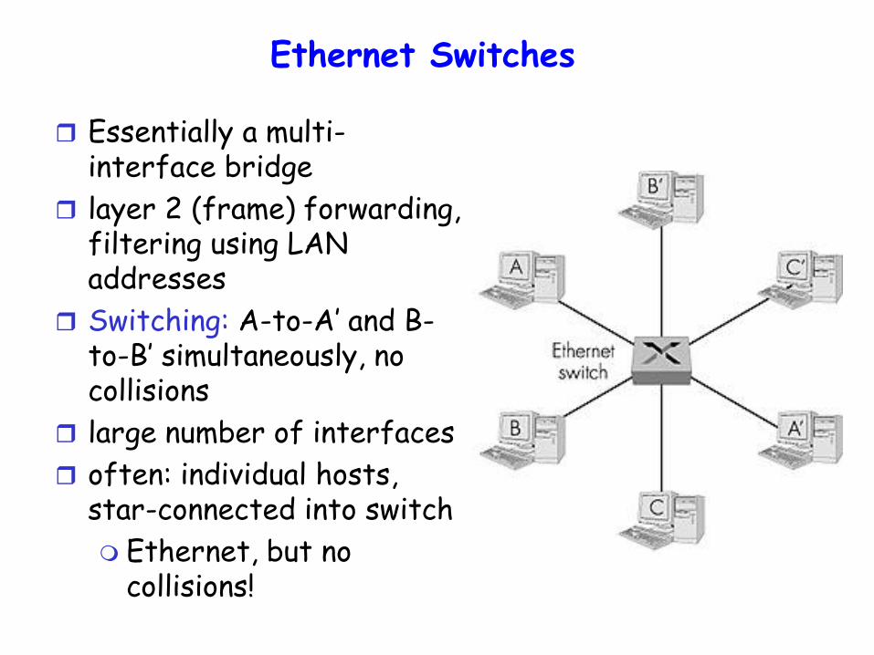
Essentially a multi-interface bridge
layer 2 (frame) forwarding, filtering using LAN addresses
Switching: A-to-A’ and B-to-B’ simultaneously, no collisions
large number of interfaces
often: individual hosts, star-connected into switch
Ethernet, but no collisions!
Ethernet Switches
cut-through switching: frame forwarded from input to output port without awaiting for assembly of entire frame slight reduction in latency
combinations of shared/dedicated, 10/100/1000 Mbps interfaces
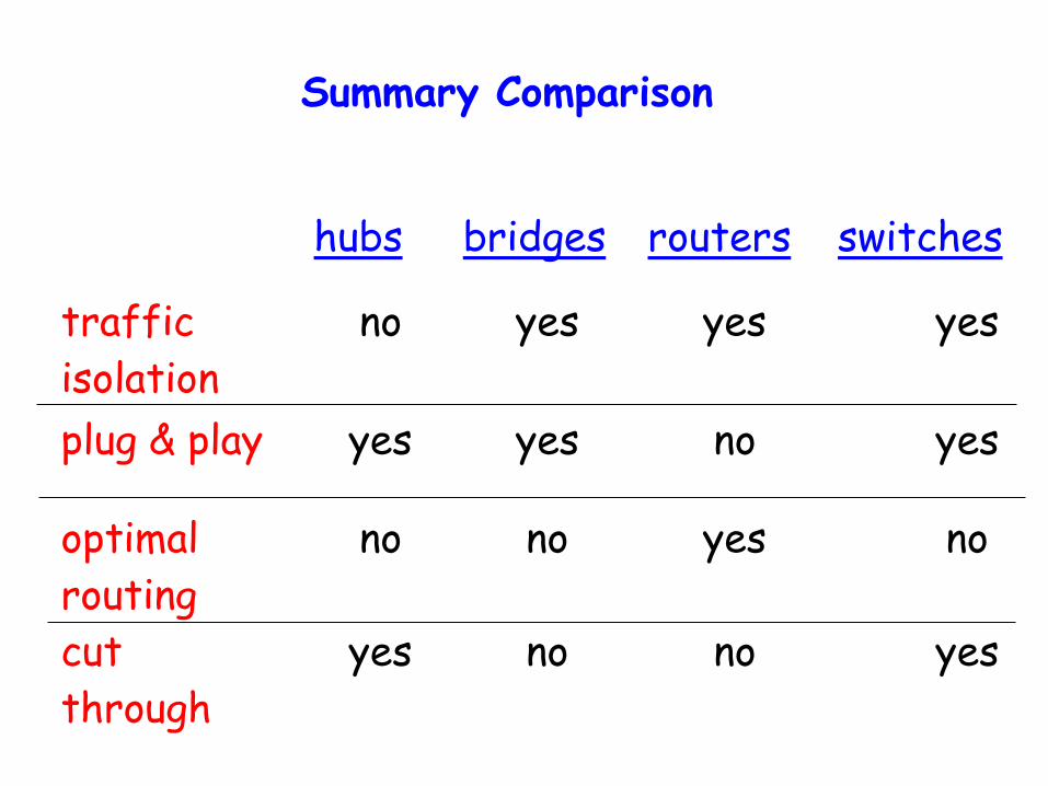
Summary Comparison
hubs bridges routers switches
traffic
isolation
no yes yes yes
plug & play yes yes no yes
optimal
routing
no no yes no
cut
through
yes no no yes

Physical
partition
Logical partition
Bridge
or
switch
VLAN 1 VLAN 2 VLAN 3
S1 7
2 3 4 5 6 1
8
9 Floor n – 1
Floor n
Floor n + 1
S2
S3
S4
S5
S6
S7
S8
S9
Virtual LAN (VLAN)
Logical partition
Bridge
or
switch
VLAN 1 VLAN 2 VLAN 3
S1 7
2 3 4 5 6 1
8
9 Floor n – 1
Floor n
Floor n + 1
S2
S3
S4
S5
S6
S7
S8
S9
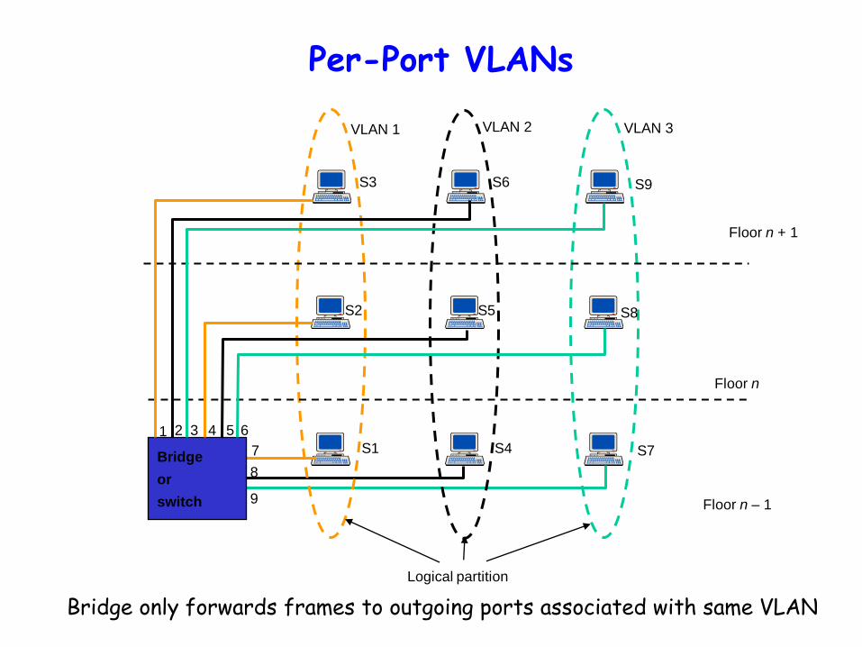
Per-Port VLANs
Bridge only forwards frames to outgoing ports associated with same VLAN

Tagged VLANs
More flexible than Port-based VLANs
Insert VLAN tag after source MAC address in each frame VLAN protocol ID + tag
VLAN-aware bridge forwards frames to outgoing ports
according to VLAN ID
VLAN ID can be associated with a port statically through configuration or dynamically through bridge learning
IEEE 802.1q
Related Documents