Lecture notes to Stock and Watson chapter 4 - UiO

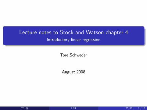
Lecture notes to Stock and Watson chapter 4Introductory linear regression

Tore Schweder

August 2008

TS () LN3 25/08 1 / 13

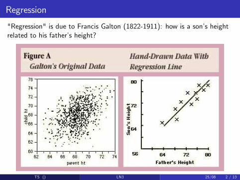
Regression

"Regression" is due to Francis Galton (1822-1911): how is a son�s heightrelated to his father�s height?

TS () LN3 25/08 2 / 13

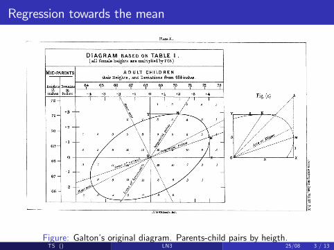
Regression towards the mean

Figure: Galton�s original diagram. Parents-child pairs by heigth.TS () LN3 25/08 3 / 13

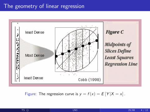
The geometry of linear regression

Figure: The regression curve is y = f (x) = E [Y jX = x ] .

TS () LN3 25/08 4 / 13

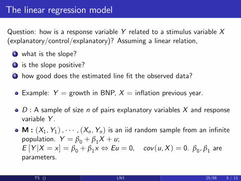
The linear regression model

Question: how is a response variable Y related to a stimulus variable X(explanatory/control/explanatory)? Assuming a linear relation,

1 what is the slope?2 is the slope positive?3 how good does the estimated line �t the observed data?

Example: Y = growth in BNP, X = in�ation previous year.

D : A sample of size n of pairs explanatory variables X and responsevariable Y .

M : (X1,Y1) , � � � , (Xn,Yn) is an iid random sample from an in�nitepopulation. Y = β0 + β1X + u;E [Y jX = x ] = β0 + β1x , Eu = 0, cov(u,X ) = 0. β0, β1 areparameters.

TS () LN3 25/08 5 / 13

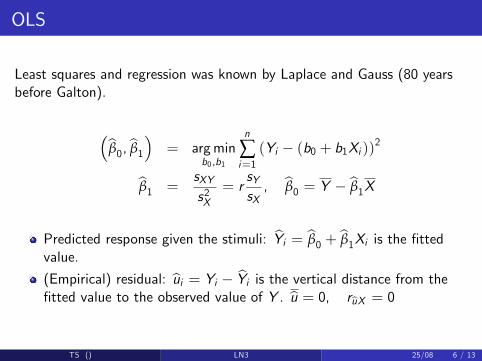
OLS

Least squares and regression was known by Laplace and Gauss (80 yearsbefore Galton).

�bβ0, bβ1� = argminb0,b1

n

∑i=1(Yi � (b0 + b1Xi ))2

bβ1 =sXYs2X

= rsYsX, bβ0 = Y � bβ1X

Predicted response given the stimuli: bYi = bβ0 + bβ1Xi is the �ttedvalue.

(Empirical) residual: bui = Yi � bYi is the vertical distance from the�tted value to the observed value of Y . bu = 0, rbuX = 0

TS () LN3 25/08 6 / 13

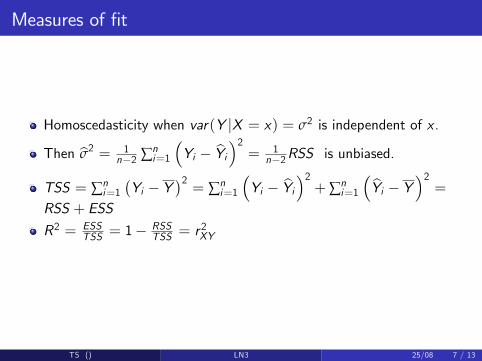
Measures of �t

Homoscedasticity when var(Y jX = x) = σ2 is independent of x .

Then bσ2 = 1n�2 ∑n

i=1

�Yi � bYi�2 = 1

n�2RSS is unbiased.

TSS = ∑ni=1

�Yi � Y

�2= ∑n

i=1

�Yi � bYi�2 +∑n

i=1

�bYi � Y �2 =RSS + ESS

R2 = ESSTSS = 1�

RSSTSS = r

2XY

TS () LN3 25/08 7 / 13

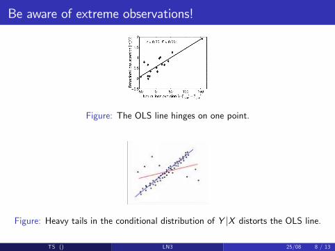
Be aware of extreme observations!

Figure: The OLS line hinges on one point.

Figure: Heavy tails in the conditional distribution of Y jX distorts the OLS line.

TS () LN3 25/08 8 / 13

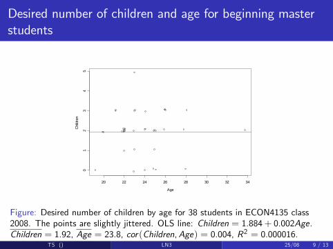
Desired number of children and age for beginning masterstudents

Age

Chi

ldre

n

20 22 24 26 28 30 32 34

01

23

45

Figure: Desired number of children by age for 38 students in ECON4135 class2008. The points are slightly jittered. OLS line: Children = 1.884+ 0.002Age.Children = 1.92, Age = 23.8, cor(Children,Age) = 0.004, R2 = 0.000016.

TS () LN3 25/08 9 / 13

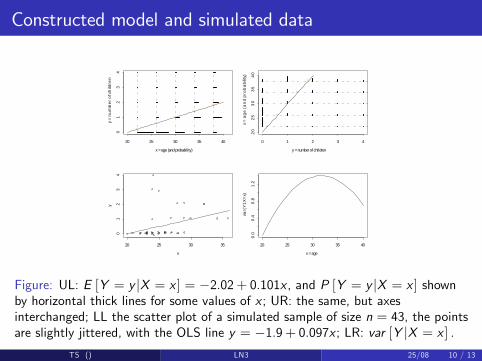
Constructed model and simulated data

x = age (and probability)

y =

nu

mb

er

of c

hild

ren

20 25 30 35 40

01

23

4

y = number of children

x =

ag

e (a

nd

pro

ba

bili

ty)

0 1 2 3 4

20

25

30

35

40

x

y

20 25 30 35

01

23

4

x = age

var(

Y1X

=x)

20 25 30 35 400

.00

.40

.81

.2

Figure: UL: E [Y = y jX = x ] = �2.02+ 0.101x , and P [Y = y jX = x ] shownby horizontal thick lines for some values of x ; UR: the same, but axesinterchanged; LL the scatter plot of a simulated sample of size n = 43, the pointsare slightly jittered, with the OLS line y = �1.9+ 0.097x ; LR: var [Y jX = x ] .

TS () LN3 25/08 10 / 13

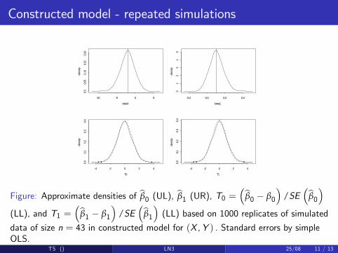
Constructed model - repeated simulations

beta0

dens

ity

10 5 0 5

0.0

0.05

0.10

0.15

0.20

beta1

dens

ity

0.2 0.0 0.2 0.4

01

23

45

T0

dens

ity

4 2 0 2 4

0.0

0.1

0.2

0.3

0.4

T1de

nsity

4 2 0 2 4

0.0

0.1

0.2

0.3

0.4

Figure: Approximate densities of bβ0 (UL), bβ1 (UR), T0 = �bβ0 � β0

�/SE

�bβ0�(LL), and T1 =

�bβ1 � β1

�/SE

�bβ1� (LL) based on 1000 replicates of simulateddata of size n = 43 in constructed model for (X ,Y ) . Standard errors by simpleOLS.

TS () LN3 25/08 11 / 13

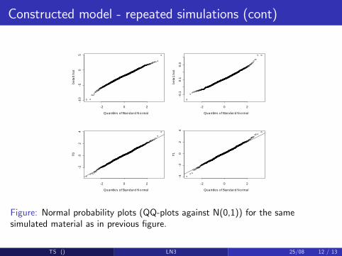
Constructed model - repeated simulations (cont)

Quantiles of Standard N ormal

beta

0.ha

t

2 0 2

10

50

5


beta

1.ha

t

2 0 2

0.1

0.1

0.3


T0

2 0 2

20

24


T1

2 0 24

20

24

Figure: Normal probability plots (QQ-plots against N(0,1)) for the samesimulated material as in previous �gure.

TS () LN3 25/08 12 / 13

Problems to be done in class

SW: 4.3

TS () LN3 25/08 13 / 13

Lecture notes to Stock and Watson chapter 4 - UiO

Documents