Lecture Notes on Nonlinear Optics Fredrik Jonsson Lectures presented at the Royal Institute of Technology Department of Laser Physics and Quantum Optics January 8 – March 24, 2003

Welcome message from author
This document is posted to help you gain knowledge. Please leave a comment to let me know what you think about it! Share it to your friends and learn new things together.
Transcript

Lecture Notes on
Nonlinear Optics
Fredrik Jonsson
Lectures presented at the Royal Institute of Technology
Department of Laser Physics and Quantum Optics
January 8 – March 24, 2003
Lecture Notes on Nonlinear OpticsNonlinear Optics (5A5513, 5p for advanced undergraduate and doctoral students)Course given at the Royal Institute of Technology,Department of Laser Physics and Quantum OpticsSE–106 91, Stockholm, SwedenJanuary 8 – March 24, 2003
Author and lecturer:Fredrik JonssonProximion Fiber Optics ABSE-164 40, KistaSweden
The texts and figures in this lecture series was typeset by the author in 10/12/16 pt ComputerModern typeface using plain TEX and METAPOST.
This document is electronically available at the homepage of the Library of the Royal Institute ofTechnology, at http://www.lib.kth.se.
Copyright c© Fredrik Jonsson 2003
All rights reserved. No part of this publication may be reproduced, stored in a retrieval system,or transmitted, in any form, or by any means, electronic, mechanical, photo-copying, recording, orotherwise, without the prior consent of the author.
ISBN 91-7283-517-6TRITA-FYS 2003:26ISSN 0280-316XISRN KTH/FYS/- - 03:26 - - SEPrinted on July 7, 2003
TEX is a trademark of the American Mathematical Society
ii

Contents
i. Structure of the courseii. Errata for Butcher and Cotter’s The Elements of Nonlinear Opticsiii. Notes on the “Butcher and Cotter convention” in nonlinear opticsiv. Recommended reference literature in nonlinear optics
Lecture 11. The contents of the course2. Examples of applications of nonlinear optics3. A brief history of nonlinear optics4. Outline for calculations of polarization densities
4.1 Metals and plasmas4.2 Dielectrics
5. Introduction to nonlinear dynamical systems6. The anharmonic oscillator
Lecture 21. Nonlinear polarization density2. Symmetries in nonlinear optics
2.1 Intrinsic permutation symmetry2.2 Overall permutation symmetry2.3 Kleinman symmetry2.4 Spatial symmetries
3. Conditions for observing nonlinear optical interactions4. Phenomenological description of the susceptibility tensors5. Linear polarization response function6. Quadratic polarization response function7. Higher order polarization response functions
Lecture 31. Susceptibility tensors in the frequency domain2. First order susceptibility tensor3. Second order susceptibility tensor4. Higher order susceptibility tensors5. Monochromatic fields6. Convention for description of nonlinear optical polarization7. Note on the complex representation of the optical field8. Example: Optical Kerr-effect
Lecture 41. The Truth of polarization densitites2. Outline3. Quantum mechanics4. Perturbation analysis of the density operator5. The interaction picture6. The first order polarization density7. The second order polarization density
Lecture 51. The second order polarization density2. Higher order polarization densities3. Assembly of independent molecules
iii

Lecture 61. Assembly of independent molecules2. First order electric susceptibility3. Overall permutation symmetry of first order susceptibility4. Second order electric susceptibility5. Overall permutation symmetry of second order susceptibility
Lecture 71. Motivation for analysis of susceptibilities in rotated coordinate systems2. Optical properties in rotated coordinate frames
2.1 First order polarization density in rotated coordinate frames2.2 Second order polarization density in rotated coordinate frames2.3 Higher order polarization densities in rotated coordinate frames
3. Crystallographic point symmetry groups4. Schonflies notation for the non-cubic crystallographic point groups5. Neumann’s principle6. Inversion properties7. Euler angles8. Example of the direct inspection technique applied to tetragonal media
8.1 Does the 422 point symmetry group possess inversion symmetry?8.2 Step one - Point symmetry under twofold rotation around the x-axis8.3 Step two - Point symmetry under fourfold rotation around the z-axis
Lecture 81. Wave propagation
1.1 Maxwell’s equations1.2 Constitutive relations
2. Two frequent assumptions in nonlinear optics3. The wave equation4. The wave equation in frequency domain (optional)5. Quasimonochromatic light - Time dependent problems6. Three practical approximations7. Monochromatic light
7.1 Monochromatic optical field7.2 Polarization density induced by monochromatic optical field
8. Monochromatic light - Time independent problems9. Example I: Optical Kerr-effect - Time independent case
10. Example II: Optical Kerr-effect - Time dependent case
Lecture 91. General process for solving problems in nonlinear optics2. Formulation of the exercises
2.1 Second harmonic generation in negative uniaxial media2.2 Optical Kerr-effect – continuous wave case
3. Second harmonic generation3.1 The optical interaction3.2 Symmetries of the medium3.3 Additional symmetries3.4 The polarization density3.5 The wave equation3.6 Boundary conditions3.7 Solving the wave equation
4. Optical Kerr-effect - Field corrected refractive index4.1 The optical interaction
iv

4.2 Symmetries of the medium4.3 Additional symmetries4.4 The polarization density4.5 The wave equation – Time independent case4.6 Boundary conditions – Time independent case4.7 Solving the wave equation – Time independent case
Lecture 101. What are solitons?2. Classes of solitons
2.1 Bright temporal envelope solitons2.2 Dark temporal envelope solitons2.3 Spatial solitons
3. The normalized nonlinear Schrodinger equation for temporal solitons3.1 The effect of dispersion3.2 The effect of a nonlinear refractive index3.3 The basic idea behind temporal solitons3.4 Normalization of the nonlinear Schrodinger equation
4. Spatial solitons5. Mathematical equivalence between temporal and spatial solitons6. Soliton solutions7. General travelling wave solutions8. Soliton interactions9. Dependence on initial conditions
Lecture 111. Singularities of non-resonant susceptibilities2. Modification of the Hamiltonian for resonant interaction3. Phenomenological representation of relaxation processes4. Perturbation analysis of weakly resonant interactions5. Validity of perturbation analysis of the polarization density6. The two-level system
6.1 Terms involving the thermal equilibrium Hamiltonian6.2 Terms involving the interaction Hamiltonian6.3 Terms involving relaxation processes
7. The rotating-wave approximation8. The Bloch equations9. The resulting electric polarization density of the medium
Lecture 121. Recapitulation of the Bloch equations for two-level systems2. The resulting electric polarization density of the medium3. The vector model of the Bloch equations4. Transient build-up at exact resonance as the optical field is switched on
4.1 The case T1 T2 – Longitudinal relaxation slower than transverse relaxation4.2 The case T1 ≈ T2 – Longitudinal relaxation approximately equal to transverse relaxation
5. Transient build-up at off-resonance as the optical field is switched on6. Transient decay for a process tuned to exact resonance
6.1 The case T1 T2 – Longitudinal relaxation slower than transverse relaxation6.2 The case T1 ≈ T2 – Longitudinal relaxation approximately equal to transverse relaxation
7. Transient decay for a slightly off-resonant process7.1 The case T1 T2 – Longitudinal relaxation slower than transverse relaxation7.2 The case T1 ≈ T2 – Longitudinal relaxation approximately equal to transverse relaxation
8. Transient decay for a far off-resonant process
v

8.1 The case T1 T2 – Longitudinal relaxation slower than transverse relaxation8.2 The case T1 ≈ T2 – Longitudinal relaxation approximately equal to transverse relaxation8.3 The case T1 T2 – Longitudinal relaxation faster than transverse relaxation
9. The connection between the Bloch equations and the susceptibility9.1 The intensity-dependent refractive index in the susceptibility formalism9.2 The intensity-dependent refractive index in the Bloch-vector formalism
10. Summary of the Bloch and susceptibility polarization densities11. Appendix: Notes on the numerical solution to the Bloch equations
Home Assignments1. Spring model for the anharmonic oscillator2. Review of quantum mechanics – The density matrix3. Nonlinear optics of the hydrogen atom4. Neumann’s principle in linear optics5. Neumann’s principle in nonlinear optics6. Review of quantum mechanics – The resonant two-level system7. Nonlinear optics of silica8. The Bloch equation9. Vector model for the Bloch equation10. Optical bistability11. Optical solitons12. Third harmonic generation in isotropic media13. The degeneracy factor14. Electro-optic phase modulation – The Pockels effect
vi

Nonlinear Optics 5A5513 (2003)
Structure of the course
Time dep. Schrodinger eqn.
ihdψdt = Hψ
Electric dipolar Hamiltonian
H(ed)I = −µαEα(r, t)
Elec. quadrupolar Hamiltonian
H(eq)I = −qαβ∂βEα(r, t)
Magnetic dipolar Hamiltonian
H(md)I = −mαBα(r, t)
Crystallographic point
symmetry class
Spatial symmetry
(§5.3)
Neumann’s principle
(§5.3.1)
Time reversal symmetry
(§5.2)
Maxwell’s equations
(§7.1.1–7.1.3)
Matrix representaion
rαab = 〈a|rα|b〉The density operator
(§3.1–3.6)
(ihdρdt = [H, ρ]
)
Perturbation analysis
(§3.7)
Susceptibility tensors,
general form (§4.3, §4.5)
Intrinsic permut. symmetry
(§2.1, §4.2)(Causality)
Overall permut. symmetry
(§4.3, §5.1.1)
Unsold approximation
(§4.7.2)
Susceptibility tensors,
reduced set (§5.3, App. 3)
(Pα(r, t) = ε0(χ
(1)αβEβ + χ
(2)αβγEβEγ + . . .)
)
Born-Oppenheimer
approx. (§4.5.4)
Description of relaxation
[HR, ρ]ab = −ihΓρab (§6.2.5)
The Bloch equation
(§6.2.5–6.3.2, §6.4)
Rotating wave approx.
(§6.2.3)
Optical Stark effect
(§6.3.3)
Inhomogeneous broadening
(§6.3.4)
Matrix elements ρab(t)
of density operator
(Pα(r, t) = NeTr[rαρ]
)
Magnetization
Mα(r, t)
Polarization density
Pα(r, t)
Electromagnetic wave
propagation
Slowly varying envelope
approximation (§7.1.4)
Multiple scales
(phase matching)
Invariants of motion
(classical mechanics)
Inverse scattering
transform (IST)
...
Linear refractive index
(§4.3.1, §6.3.1)
Linear absorption
(§4.5, §6.3.1)
1st order effects
OPG, OPO
(§7.2.2)
SHG
(§7.2.1)
Millers delta rule
(§4.7.3)
2nd order effects
Optical bistability
(§2.6)
THG
(§5.3.4)
Raman scattering
(§6.5, §4.5.2)
3rd order effects
Phase conjugation
(§7.4)
Brillouin scattering
(§2.3.3)
Optical solitons
(§7.5)
3rd order effects
Microscopic description
Macroscopic description
Non-resonant and weaklyresonant interactions Resonant interactions
Non-resonant interactions
Mathematical tools
Applications
1

Nonlinear Optics 5A5513 (2003) Lecture Notes on Nonlinear Optics
2

Lecture Notes on Nonlinear Optics Nonlinear Optics 5A5513 (2003)
Errors in The Elements of Nonlinear Optics (1991)by Paul Butcher and David Cotter
Errata written by Fredrik Jonsson
Updated as of March 16, 2003
Please send additions or corrections to [email protected]
Below follows a listing of errors found in P. N. Butcher and D. Cotters book The Elements ofNonlinear Optics (Cambridge University Press, Cambridge, 1991). Being a summary of the notesI have made in my personal copy of the book since June 1996, this list should by no means beconsidered as any kind of “official” list of errors, but rather as an attempt to collect the (ratherfew) misprints in the text. In the list, not only typographical misprints, but also some inconsequentnotations – which do not alter the described theory – are included.
p. 15 [lines 14 and 16 ] In order not to introduce any ambiguity of the multiple arguments of thesymmetric and antisymmetric parts, the arguments (t; τ1, τ2) should be explicitly written in theleft-hand sides of the equations.
p. 15 [line 18 ] “. . . dummy variables ατ1 and βτ2.” should be replaced by “. . . dummy variables(α, τ1) and (β, τ2).”, following the notation as used later in, for example, §2.3.2 and §4.3.1.p. 49 [line 31 ] H1(t) should be replaced by HI(t).
p. 54 [lines 3, 4, and 6 ] In Eq. (3.80), the upper limit of integration t1 should be replaced by τ1.
p. 54 [lines 8 and 24 ] In Eqs. (3.81) and (3.82), the upper limits of integration t1 and tn−1 shouldbe replaced by τ1 and τn−1, respectively.
p. 60 [line 24 ] The sentence “To achieve this end we . . .” should be replaced by “To achieve thiswe . . .”
p. 66 [line 11 ] In the right hand side of Eq. (4.49), one should in order not to cause confusion withthe Einstein convention of summation over repeated indices explicitly state that no summation isimplied, and hence the equation should be written as
H0ui(Θ) = Eiui(Θ). (no sum) (4.49)
using the common notation as used in tensor calculus.
p. 67 [line 6 ] “. . . express the the unperturbed . . .” should be replaced by “. . . express the unper-turbed . . .”
p. 72 [line 15 ] “(α, ω1)” should be replaced by “(α, ω1)”.
p. 72 [last line ] “. . . of this type, one of which is an identity.” should be replaced by “. . . of thistype, of which one is an identity.”
p. 86 [line 4 ] In Eq. (4.103), “· · · ft(ωn · en〉” should be replaced by “· · · ft(ωn) · en〉”.p. 93 [lines 12–13 ] Strictly speaking, the real part of the susceptibility χ(1)(−ωσ;ω) is not pro-portional to the refractive index n(ω), but rather to n2(ω) − 1.
p. 97 [lines 15 and 20 ] Strictly speaking, Ωfg is the transition angular frequency, and does nothave the physical dimension of energy; therefore replace “Ωfg” in lines 15 and 20 by “~Ωfg”.
p. 106 [line 9 ] In the first term of Eq. (4.128), the summation should be performed over index jrather than index i, i. e. replace
∑i pj by
∑j pj .
p. 132 [line 8 ] In Eq. (5.30), “Eiui(Θ)” should be replaced by “Eiui(Θ) (no sum)”.
p. 132 [line 25 ] “ρ0(a) = η exp(−Ea/kT )” should be replaced by “ρ0(a) = η exp(−Ea/kT )”.
3

Nonlinear Optics 5A5513 (2003) Lecture Notes on Nonlinear Optics
p. 136 [line 19 ] In Eq. (5.43), “χua(1)(−ω, ω)” should be replaced by “χ(1)ua (−ω, ω)”.
p. 159 [line 13 ] In the left-hand side of Eq. (6.33), the Hamiltonian H0 describing the systemis a quantum-mechanical operator, while in the right-hand side, the matrix representation of thecorresponding elements 〈m|H0|n〉 = δmnEn in the energy representation appears. In order toovercome this inconsistency, Eq. (6.33) should (in analogy with, for example, Eq. (6.31) for thematrix elements of the density operator) be replaced by either
(〈a|H0|a〉 〈a|H0|b〉〈b|H0|a〉 〈b|H0|b〉
)=
(Ea 00 Eb
),
or ([H0]aa [H0]ab[H0]ba [H0]bb
)=
(Ea 00 Eb
).
p. 160 [line 2 ] In the left-hand side of Eq. (6.34), the Hamiltonian HI(t) is a quantum-mechanicaloperator, while in the right-hand side, the matrix representation of its scalar elements 〈a|HI(t)|b〉appears. (The same inconsistency appear in Eq. (6.33).) In order to overcome this inconsistency,Eq. (6.34) should (in analogy with, for example, Eq. (6.31) for the matrix elements of the densityoperator) be replaced by either
(〈a|HI(t)|a〉 〈a|HI(t)|b〉〈b|HI(t)|a〉 〈b|HI(t)|b〉
)=
(δEa −erab · E(t)
−erba · E(t) δEb
),
or ([HI(t)]aa [HI(t)]ab[HI(t)]ba [HI(t)]bb
)=
(δEa −erab · E(t)
−erba · E(t) δEb
).
p. 164 [line 15 ] In Eq. (6.49), “i~(1 − ρbb)/Tb” should be replaced by “i~(1 − ρaa)/Tb”.†p. 203 [lines 32–33 ] “Fig. 4.3” should be replaced by “Fig. 4.4(a)”.
p. 215 [line 11 ] In Eq. (7.14),
. . . = µ0
∫ ∞
−∞
dω′(ω + ω′)2 · · ·
should be replaced by
. . . =1
c2
∫ ∞
−∞
dω′(ω + ω′)2 · · ·
p. 220 [section 7.2.1 ] In the example of second harmonic generation, the wave equation (7.26)is given without any explanation of which point symmetry class it applies to, and hence it isfrom the text virtually impossible to relate the effective nonlinear parameters to the elements of
χ(2)µαβ(−ωσ;ω, ω).
p. 234 [line 31 ] In Eq. (7.45), “. . . = iq∗E∗3 >” should be replaced by “. . . = iq∗E∗
3”.
p. 240 [line 6 ] In the first line of Eq. (7.55), there is an ambiguity of the denominator, as well asan erroneous dispersion term, and the equation
u = τ√n2ω/c|d2k/dω2|2E
should be replaced byu = τ
√n2ω/(c|d2k/dω2|)E.
(The other lines of Eq. (7.55) are correct.)
† Cf. M. D. Levenson and S. S. Kano, Introduction to Nonlinear Laser Spectroscopy (AcademicPress, New York, 1988), p. 33, Eqs. (2.3.1)–(2.3.2).
4
Lecture Notes on Nonlinear Optics Nonlinear Optics 5A5513 (2003)
p. 241 [line 30 ] The fundamental bright soliton solution to the nonlinear Schrodinger equationshould yield “u(ζ, s) = sech(s) exp(iζ/2)”, that is to say, without any minus sign in the exponential.
p. 251 [line 6 ] In Eq. (8.5), there is parenthesis mismatch in both right- and lefthand sides;
f0[(En(k)] = exp[En(k) − EF]/kT + 1−1
should be replaced byf0[En(k)] = exp[(En(k) − EF)/kT ] + 1−1.
p. 252 [line 6 ] In Eq. (8.7), nph(ωs(q)) should be replaced by nph[ωs(q)], in order to follow thefunctional style of notation as used in, for example, Eq. (8.5).
p. 253 [line 20 ] In Eq. (8.11), insert a “]” after En(k).
p. 298 [Table A3.2 ] “. . . no centre of symmetry . . .” should be replaced by “. . . no centre ofinversion . . .”.
p. 317 [lines 1, 9, and 24 ] In Appendix 9, there is an inconsistency in the notation for the polar-isation density and the electric dipole operator, as compared to the one used in Chapters 3 and4. While PD, PQ, and MD in Eq. (A9.1) (and in line 9 on the same page) denote the all-classicalelectric dipolar, electric quadrupolar and magnetic dipolar polarization densities of the medium,they in Eqs. (A9.6) and (A9.7) clearly denote quantum-mechanical operators. In order to overcomethis inconsistency in notation, which in addition gives a wrong answer if properly inserted into theperturbation calculus etc., one should chose either of the conventions. By choosing PD, PQ, andMD to denote the corresponding quantum-mechanical operators, which seem to be the easiest wayof correcting this inconsistency, the following corrections to the text should be made:
[line 1P = PD + PQ, M = MD, (A9.1)
should be replaced byP = 〈PD〉 + 〈PQ〉, M = 〈MD〉, (A9.1)
[line 9 Remove “PD” or replace with “〈PD〉”.[line 24 Somewhere in Appendix 9, there should be a clarifying statement that the nabla
operator appearing in Eq. (A9.7) only is operating on the all-classical, macroscopic electric fieldof the light, and hence should be regarded as a classical vector when evaluating the quantum-mechanical trace that is involved in the expectation value of, for example, the corrected form ofEq. (A9.1).
p. 318 [line 12 ] “M << H” should be replaced by “|M| |H|”.p. 318 [line 23 ] “ej · er + ik · q · ej + m · (k× ej)/ω” should be replaced by the same expression,though with each term divided by e.
p. 333 [line 5 ] In reference Manley, J. M. and Rowe, H. E. (1956), the page numbers should yield904 – 14.
p. 334 [line 44 ] “Terhune, R. W. and Weinburger, D. A. . . .” should be replaced by “Terhune,R. W. and Weinberger, D. A. . . .”.
5

Nonlinear Optics 5A5513 (2003) Lecture Notes on Nonlinear Optics
6

Nonlinear Optics 5A5513 (2003)
Notes on the “Butcher and Cotter convention” in nonlinear optics
Convention for description of nonlinear optical polarization
As a “recipe” in theoretical nonlinear optics, Butcher and Cotter provide a very useful conventionwhich is well worth to hold on to. For a superposition of monochromatic waves, and by invokingthe general property of the intrinsic permutation symmetry, the monochromatic form of the nthorder polarization density can be written as
(P (n)ωσ
)µ = ε0∑
α1
· · ·∑
αn
∑
ω
K(−ωσ;ω1, . . . , ωn)χ(n)µα1···αn
(−ωσ;ω1, . . . , ωn)(Eω1)α1
· · · (Eωn)αn
.
(1)The first summations in Eq. (1), over α1, . . . , αn, is simply an explicit way of stating that theEinstein convention of summation over repeated indices holds. The summation sign
∑ω, however,
serves as a reminder that the expression that follows is to be summed over all distinct sets ofω1, . . . , ωn. Because of the intrinsic permutation symmetry, the frequency arguments appearing inEq. (1) may be written in arbitrary order.
By “all distinct sets of ω1, . . . , ωn”, we here mean that the summation is to be performed, asfor example in the case of optical Kerr-effect, over the single set of nonlinear susceptibilities thatcontribute to a certain angular frequency as (−ω;ω, ω,−ω) or (−ω;ω,−ω, ω) or (−ω;−ω, ω, ω).In this example, each of the combinations are considered as distinct, and it is left as an arbitarychoice which one of these sets that are most convenient to use (this is simply a matter of choosingnotation, and does not by any means change the description of the interaction).
In Eq. (1), the degeneracy factor K is formally described as
K(−ωσ;ω1, . . . , ωn) = 2l+m−np
wherep = the number of distinct permutations of ω1, ω2, . . . , ω1,
n = the order of the nonlinearity,
m = the number of angular frequencies ωk that are zero, and
l =
1, if ωσ 6= 0,0, otherwise.
In other words, m is the number of DC electric fields present, and l = 0 if the nonlinearity we areanalyzing gives a static, DC, polarization density, such as in the previously (in the spring model)described case of optical rectification in the presence of second harmonic fields (SHG).
A list of frequently encountered nonlinear phenomena in nonlinear optics, including the degen-eracy factors as conforming to the above convention, is given in Butcher and Cotters book, Table2.1, on page 26.
Note on the complex representation of the optical field
Since the observable electric field of the light, in Butcher and Cotters notation taken as
E(r, t) =1
2
∑
ωk≥0
[Eωkexp(−iωkt) + E∗
ωkexp(iωkt)],
is a real-valued quantity, it follows that negative frequencies in the complex notation should beinterpreted as the complex conjugate of the respective field component, or
E−ωk= E∗
ωk.
7
Nonlinear Optics 5A5513 (2003)
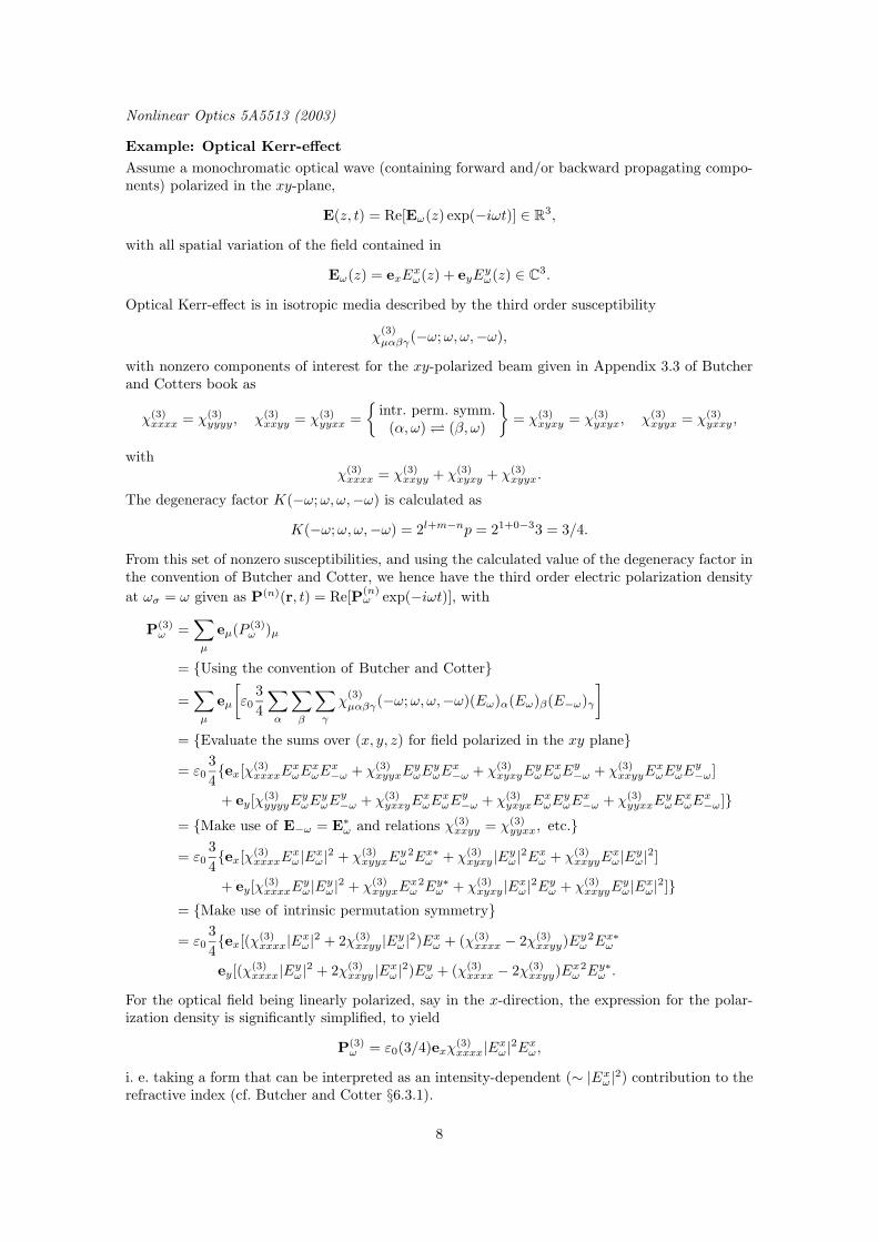
Example: Optical Kerr-effect
Assume a monochromatic optical wave (containing forward and/or backward propagating compo-nents) polarized in the xy-plane,
E(z, t) = Re[Eω(z) exp(−iωt)] ∈ R3,
with all spatial variation of the field contained in
Eω(z) = exExω(z) + eyE
yω(z) ∈ C
3.
Optical Kerr-effect is in isotropic media described by the third order susceptibility
χ(3)µαβγ(−ω;ω, ω,−ω),
with nonzero components of interest for the xy-polarized beam given in Appendix 3.3 of Butcherand Cotters book as
χ(3)xxxx = χ(3)
yyyy , χ(3)xxyy = χ(3)
yyxx =
intr. perm. symm.
(α, ω) (β, ω)
= χ(3)
xyxy = χ(3)yxyx, χ(3)
xyyx = χ(3)yxxy ,
withχ(3)xxxx = χ(3)
xxyy + χ(3)xyxy + χ(3)
xyyx.
The degeneracy factor K(−ω;ω, ω,−ω) is calculated as
K(−ω;ω, ω,−ω) = 2l+m−np = 21+0−33 = 3/4.
From this set of nonzero susceptibilities, and using the calculated value of the degeneracy factor inthe convention of Butcher and Cotter, we hence have the third order electric polarization density
at ωσ = ω given as P(n)(r, t) = Re[P(n)ω exp(−iωt)], with
P(3)ω =
∑
µ
eµ(P(3)ω )µ
= Using the convention of Butcher and Cotter
=∑
µ
eµ
[ε0
3
4
∑
α
∑
β
∑
γ
χ(3)µαβγ(−ω;ω, ω,−ω)(Eω)α(Eω)β(E−ω)γ
]
= Evaluate the sums over (x, y, z) for field polarized in the xy plane
= ε03
4ex[χ(3)
xxxxExωE
xωE
x−ω + χ(3)
xyyxEyωE
yωE
x−ω + χ(3)
xyxyEyωE
xωE
y−ω + χ(3)
xxyyExωE
yωE
y−ω]
+ ey[χ(3)yyyyE
yωE
yωE
y−ω + χ(3)
yxxyExωE
xωE
y−ω + χ(3)
yxyxExωE
yωE
x−ω + χ(3)
yyxxEyωE
xωE
x−ω]
= Make use of E−ω = E∗ω and relations χ(3)
xxyy = χ(3)yyxx, etc.
= ε03
4ex[χ(3)
xxxxExω|Exω|2 + χ(3)
xyyxEyω
2Ex∗ω + χ(3)xyxy |Eyω|2Exω + χ(3)
xxyyExω|Eyω|2]
+ ey[χ(3)xxxxE
yω|Eyω|2 + χ(3)
xyyxExω
2Ey∗ω + χ(3)xyxy |Exω|2Eyω + χ(3)
xxyyEyω|Exω|2]
= Make use of intrinsic permutation symmetry
= ε03
4ex[(χ(3)
xxxx|Exω|2 + 2χ(3)xxyy |Eyω|2)Exω + (χ(3)
xxxx − 2χ(3)xxyy)E
yω
2Ex∗ω
ey[(χ(3)xxxx|Eyω|2 + 2χ(3)
xxyy |Exω|2)Eyω + (χ(3)xxxx − 2χ(3)
xxyy)Exω
2Ey∗ω .
For the optical field being linearly polarized, say in the x-direction, the expression for the polar-ization density is significantly simplified, to yield
P(3)ω = ε0(3/4)exχ
(3)xxxx|Exω|2Exω,
i. e. taking a form that can be interpreted as an intensity-dependent (∼ |Exω|2) contribution to the
refractive index (cf. Butcher and Cotter §6.3.1).
8

Nonlinear Optics 5A5513 (2003)
Recommended reference literature in nonlinear optics
[1] P. N. Butcher and D. Cotter, The Elements of Nonlinear Optics (Cambridge UniversityPress, Cambridge, 1991). Uses SI units throughout the text.
[2] Y. R. Shen, The Principles of Nonlinear Optics (Wiley, New York, 1984). A standard textwhich covers most of the phenomena and applications in nonlinear optics. More directedtowards the already active scientist in the field, rather than being a tutorial text. UsesGaussian units throughout the text.
[3] D. C. Hanna, M. A. Yuratich, and D. Cotter, Nonlinear Optics of Free Atoms and Molecules(Springer-Verlag, Berlin, 1979). Contains a somewhat more detailed description of electricquadrupolar contributions to nonlinear susceptibilities than otherwise usually found intextbooks in nonlinear optics. Uses SI units throughout the text.
[4] R. W. Boyd, Nonlinear Optics (Academic Press, Boston, 1992). Starting more from anatomic physics point of view, this book contains aspects on spectroscopical applications ofnonlinear optics. Uses Gaussian units throughout the text.
[5] P. Meystre and M. Sargent III, Elements of quantum optics (Springer-Verlag, Berlin, 1998),3rd ed. The title of this book might be somewhat misleading, since the book contains quitea lot of interesting discussions on nonlinear optical phenomena from a classical description.This textbook provides a strict quantum-mechanical approach to linear as well as nonlinearoptical interactions. The authors have chosen to include somewhat more classical tools ofanalysis as well, such as the Ikeda instability analysis of optical Kerr-media, and theLorenz model for the dynamics of the homogeneously broadened singlemode unidirectionalring laser, the latter leading to solutions possessing deterministic chaos. Uses SI unitsthroughout the text.
[6] A. C. Newell and J. V. Moloney, Nonlinear optics (Addison-Wesley, New York, 1992).In this book the principles of nonlinear optics are described from a more mathematicalpoint of view. Wave propagation in nonlinear optical media is covered in more detail thanin other books, and the theory of solitons is described. Contains a nice introduction tothe deterministic chaos which is an intrinsic property of some numerical solutions to thewave propagation problem in certain nonlinear optical media. The book covers the Blochequations, describing the interaction between light and matter, but does surprisingly notcover the origin of the nonlinear susceptibility tensors, even though they play a centralrole in the first chapters of the book. In the last chapter, a review of mathematical andcomputional tools that frequently are applied in nonlinear optics is presented. Uses SIunits throughout the text.
[7] N. Bloembergen Nonlinear Optics (World Scientific, London, 1996), 4th ed. Almost to beconsidered as the historical text on nonlinear optics. The first edition of this book appearedas early as 1965, just a few years after the first observations of nonlinear optical phenom-ena by Franken et al. (1961). Some of the early, pioneering papers on nonlinear optics(e. g. J. A. Armstrong, N. Bloembergen, J. Ducuing, and P. S. Pershan, Phys. Rev. 127,1918 (1962); P. A. Franken, A. E. Hill, C. W. Peters, G. Weinreich, Phys. Rev. Lett. 7,118 (1961)) are in this book extended and presented in more detail. In 1981, NicolaasBloembergen and Arthur Schawlow received the Nobel prize for their contribution to thedevelopment of laser spectroscopy, in particular using nuclear magnetic resonance (NMR).Gaussian units are used throughout the text.
9

Nonlinear Optics 5A5513 (2003) Lecture Notes on Nonlinear Optics
10

Lecture Notes on Nonlinear Optics Nonlinear Optics 5A5513 (2003)
Lecture I
11
Nonlinear Optics 5A5513 (2003) Lecture Notes on Nonlinear Optics
Lecture Notes on Nonlinear OpticsNonlinear Optics (5A5513, 5p for advanced undergraduate and doctoral students)Course given at the Royal Institute of Technology,Department of Laser Physics and Quantum OpticsSE–106 91, Stockholm, SwedenJanuary 8 – March 24, 2003
The texts and figures in this lecture series was typeset by the author in 10/12/16 pt ComputerModern typeface using plain TEX and METAPOST.
This document is electronically available at the homepage of the Library of the Royal Instituteof Technology, at http://www.lib.kth.se.
Copyright c© Fredrik Jonsson 2003
All rights reserved. No part of this publication may be reproduced, stored in a retrievalsystem, or transmitted, in any form, or by any means, electronic, mechanical, photo-copying,recording, or otherwise, without the prior consent of the author.
ISBN 91-7283-517-6TRITA-FYS 2003:26ISSN 0280-316XISRN KTH/FYS/- - 03:26 - - SEPrinted on July 7, 2003
TEX is a trademark of the American Mathematical Society
12

Nonlinear Optics 5A5513 (2003)Lecture notes
Lecture 1
Nonlinear optics is the discipline in physics in which the electric polarization density of the mediumis studied as a nonlinear function of the electromagnetic field of the light. Being a wide field ofresearch in electromagnetic wave propagation, nonlinear interaction between light and matter leadsto a wide spectrum of phenomena, such as optical frequency conversion, optical solitons, phaseconjugation, and Raman scattering. In addition, many of the analytical tools applied in nonlinearoptics are of general character, such as the perturbative techniques and symmetry considerations,and can equally well be applied in other disciplines in nonlinear dynamics.
The contents of this course
This course is intended as an introduction to the wide field of phenomena encountered in nonlinearoptics. The course covers:
• The theoretical foundation of nonlinear interaction between light and matter.• Perturbation analysis of nonlinear interaction between light and matter.• The Bloch equation and its interpretation.• Basics of soliton theory and the inverse scattering transform.
It should be emphasized that the course does not cover state-of-the-art material constantsof nonlinear optical materials, etc. but rather focus on the theoretical foundations and ideas ofnonlinear optical interactions between light and matter.
A central analytical technique in this course is the perurbation analysis, with its foundationin the analytical mechanics. This technique will in the course mainly be applied to the quantum-mechanical description of interaction between light and matter, but is central in a wide field ofcross-disciplinary physics as well. In order to give an introduction to the analytical theory ofnonlinear systems, we will therefore start with the analysis of the nonlinear equations of motionfor the mechanical pendulum.
Examples of applications of nonlinear optics
Some important applications in nonlinear optics:
• Optical parametric amplification (OPA) and oscillation (OPO), ~ωp → ~ωs + ~ωi.• Second harmonic generation (SHG), ~ω + ~ω → ~(2ω).• Third harmonic generation (THG), ~ω + ~ω + ~ω → ~(3ω).• Pockels effect, or the linear electro-optical effect (applications for optical switching).• Optical bistability (optical logics).• Optical solitons (ultra long-haul communication).
13

Nonlinear Optics 5A5513 (2003) Lecture notes 1
A brief history of nonlinear optics
Some important advances in nonlinear optics:
• Townes et al. (1960), invention of the laser.1
• Franken et al. (1961), First observation ever of nonlinear optical effects, second harmonicgeneration (SHG).2
• Terhune et al. (1962), First observation of third harmonic generation (THG).3
• E. J. Woodbury and W. K. Ng (1962), first demonstration of stimulated Raman scattering.4
• Armstrong et al. (1962), formulation of general permutation symmetry relations in nonlinearoptics.5
• A. Hasegawa and F. Tappert (1973), first theoretical prediction of soliton generation in opticalfibers.6
• H. M. Gibbs et al. (1976), first demonstration and explaination of optical bistability.7
• L. F. Mollenauer et al. (1980), first confirmation of soliton generation in optical fibers.8
Recently, many advances in nonlinear optics has been made, with a lot of efforts with fields of,for example, Bose-Einstein condensation and laser cooling; these fields are, however, a bit out offocus from the subjects of this course, which can be said to be an introduction to the 1960s and1970s advances in nonlinear optics. It should also be emphasized that many of the effects observedin nonlinear optics, such as the Raman scattering, were observed much earlier in the microwaverange.
Outline for calculations of polarization densities
Metals and plasmas
From an all-classical point-of-view, the calculation of the electric polarization density of metals andplasmas, containing a free electron gas, can be performed using the model of free charges actingunder the Lorenz force of an electromagnetic field,
med2re
dt2= −eE(t) − e
dre
dt× B(t),
where E and B are all-classical electric and magnetic fields of the electromagnetic field of the light.In forming the equation for the motion of the electron, the origin was chosen to coincide with thecenter of the nucleus.
1 Charles H. Townes was in 1964 awarded with the Nobel Prize for the invention of the ammonialaser.
2 Franken et al. detected ulvtraviolet light (λ = 347.1 nm) at twice the frequency of a ruby laserbeam (λ = 694.2 nm) when this beam traversed a quartz crystal; P. A. Franken, A. E. Hill, C. W.Peters, G. Weinreich, Phys. Rev. Lett. 7, 118 (1961). Second harmonic generation is also the firstnonlinear effect ever observed where a coherent input generates a coherent output.
3 In their experiment, Terhune et al. detected only about a thousand THG photons per pulse,at λ = 231.3 nm, corresponding to a conversion of one photon out of about 1015 photons at thefundamental wavelength at λ = 693.9 nm; R. W. Terhune, P. D. Maker, and C. M. Savage, Phys.Rev. Lett. 8, 404 (1962).
4 E. J. Woodbury and W. K. Ng, Proc. IRE 50, 2347 (1962).5 The general permutation symmetry relations of higher-order susceptibilities were published by
J. A. Armstrong, N. Bloembergen, J. Ducuing, and P. S. Pershan, Phys. Rev. 127, 1918 (1962).6 A. Hasegawa and F. Tappert, “Transmission of stationary nonliner optica pulses in dispersive
optical fibers: I, Anomalous dispersion; II Normal dispersion”, Appl. Phys. Lett. 23, 142–144and 171–172 (August 1 and 15, 1973).
7 H. M. Gibbs, S. M. McCall, and T. N. C. Venkatesan, Phys. Rev. Lett. 36, 1135 (1976).8 L. F. Mollenauer, R. H. Stolen, and J. P. Gordon, “Experimental observation of picosecond
pulse narrowing and solitons in optical fibers”, Phys. Rev. Lett. 45, 1095–1098 (September 29,1980); the first reported observation of solitons was though made in 1834 by John Scott Russell, aScottish scientist and later famous Victorian engineer and shipbuilder, while studying water wavesin the Glasgow-Edinburgh channel.
14

Lecture notes 1 Nonlinear Optics 5A5513 (2003)
Dielectrics
A very useful model used by Drude and Lorentz9 to calculate the linear electric polarization of themedium describes the electrons as harmonically bound particles.
For dielectrics in the nonlinear optical regime, as being the focus of our attention in this course,the calculation of the electric polarization density is instead performed using a nonlinear springmodel of the bound charges, here quoted for one-dimensional motion as
med2xe
dt2+ Γe
dxe
dt+ α(1)xe + α(2)x2
e + α(3)x3e + . . . = −eEx(t).
As in the previous case of metals and plasmas, in forming the equation for the motion of theelectron, the origin was also here chosen to coincide with the center of the nucleus.
This classical mechanical model will later in this lecture be applied to the derivation of thesecond-order nonlinear polarzation density of the medium.
Introduction to nonlinear dynamical systems
In this section we will, as a preamble to later analysis of quantum-mechanical systems, applyperturbation analysis to a simple mechanical system. Among the simplest nonlinear dynamicalsystems is the pendulum, for which the total mechanical energy of the system, considering thepoint of suspension as defining the level of zero potential energy, is given as the sum of the kineticand potential energy as
E = T + V =1
2m|p|2 −mgl(cosϑ− 1), (1)
where m is the mass, g the gravitation constant, l the length, and ϑ the angle of deflection of thependulum, and where p is the momentum of the point mass.
ϑ
m
l
ϕ
Figure 1. The mechanical pendulum.
From the total mechanical energy (1) of the system, the equations of motion for the point mass ishence given by Lagranges equations,10
d
dt
(∂L
∂pj
)− ∂L
∂qj= 0, j = x, y, z, (2)
where qj are the generalized coordinates, pj = qj are the components of the generalized momentum,and L = T − V is the Lagrangian of the mechanical system. In spherical coordinates (ρ, ϕ, ϑ), themomentum for the mass is given as its mass times the velocity,
p = ml(ϑeϑ + ϕ sinϑeϕ)
and the Lagrangian for the pendulum is hence given as
L =1
2m(p2ϕ + p2
ϕ) +mgl(cosϑ− 1)
=ml2
2(ϑ2 + ϕ2 sin2 ϑ) +mgl(cosϑ− 1).
9 R. Becker, Elektronen Theorie, (Teubner, Leipzig, 1933).10 Herbert Goldstein, Classical Mechanics, 2nd ed. (Addison-Wesley, Massachusetts, 1980).
15
Nonlinear Optics 5A5513 (2003) Lecture notes 1
As the Lagrangian for the pendulum is inserted into Eq. (2), the resulting equations of motion arefor qj = ϕ and ϑ obtained as
d2ϕ
dt2+
(dϕ
dt
)2
sinϕ cosϕ = 0, (3a)
andd2ϑ
dt2+ (g/l) sinϑ = 0, (3b)
respectively, where we may notice that the motion in eϕ and eϑ directions are decoupled. We mayalso notice that the equation of motion for ϕ is independent of any of the physical parametersinvolved in te Lagrangian, and the evolution of ϕ(t) in time is entirely determined by the initialconditions at some time t = t0.
In the following discussion, the focus will be on the properties of the motion of ϑ(t). Theequation of motion for the ϑ coordinate is here described by the so-called Sine-Gordon equation.11
This nonlinear differential equation is hard† to solve analytically, but if the nonlinear term isexpanded as a Taylor series around ϑ = 0,
d2ϑ
dt2+ (g/l)(ϑ− ϑ3
3!+ϑ5
5!+ . . .) = 0,
Before proceeding further with the properties of the solutions to the approximative Sine-Gordon,including various orders of nonlinearities, the general properties will now be illustrated. In order toillustrate the behaviour of the Sine-Gordon equation, we may normalize it by using the normalizedtime τ = (g/l)1/2t, giving the Sine-Gordon equation in the normalized form
d2ϑ
dτ2+ sinϑ = 0. (4)
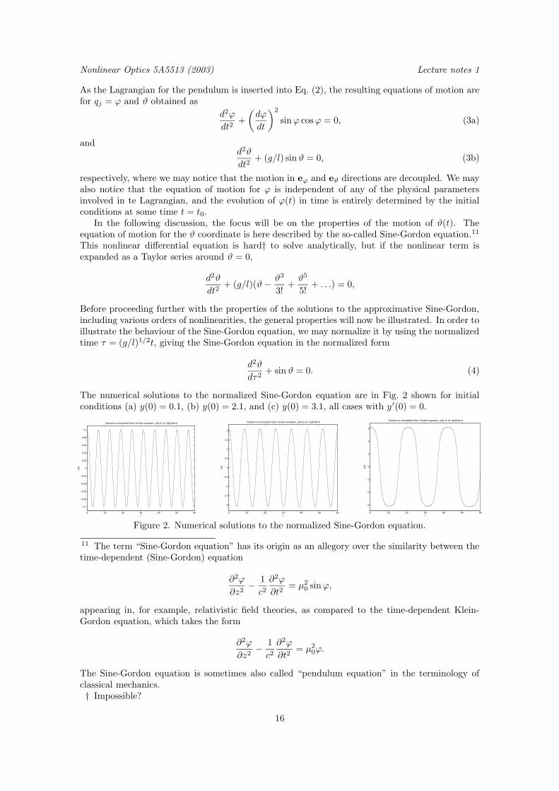
The numerical solutions to the normalized Sine-Gordon equation are in Fig. 2 shown for initialconditions (a) y(0) = 0.1, (b) y(0) = 2.1, and (c) y(0) = 3.1, all cases with y′(0) = 0.
0 10 20 30 40 50 60
−0.1
−0.08
−0.06
−0.04
−0.02
0
0.02
0.04
0.06
0.08
0.1
t
y(t)
Solution to normalized Sine−Gordon equation, y(0)=0.10, dy(0)/dt=0
0 10 20 30 40 50 60
−2
−1.5
−1
−0.5
0
0.5
1
1.5
2
t
y(t)
Solution to normalized Sine−Gordon equation, y(0)=2.10, dy(0)/dt=0
0 10 20 30 40 50 60
−3
−2
−1
0
1
2
3
t
y(t)
Solution to normalized Sine−Gordon equation, y(0)=3.10, dy(0)/dt=0
Figure 2. Numerical solutions to the normalized Sine-Gordon equation.
11 The term “Sine-Gordon equation” has its origin as an allegory over the similarity between thetime-dependent (Sine-Gordon) equation
∂2ϕ
∂z2− 1
c2∂2ϕ
∂t2= µ2
0 sinϕ,
appearing in, for example, relativistic field theories, as compared to the time-dependent Klein-Gordon equation, which takes the form
∂2ϕ
∂z2− 1
c2∂2ϕ
∂t2= µ2
0ϕ.
The Sine-Gordon equation is sometimes also called “pendulum equation” in the terminology ofclassical mechanics.† Impossible?
16
Lecture notes 1 Nonlinear Optics 5A5513 (2003)
First of all, we may consider the linear case, for which the approximation sinϑ ≈ ϑ holds. Forthis case, the Sine-Gordon equation (4) hence reduces to the one-dimensional linear wave-equation,with solutions ϑ = A sin((g/l)1/2(t − t0)). As seen in the frequency domain, this solution gives adelta peak at ω = (g/l)1/2 in the power spectrum |ϑ(ω)|2, with no other frequency componentspresent. However, if we include the nonlinearities, the previous sine-wave solution will tend toflatten at the peaks, as well as increase in period, and this changes the power spectrum to bebroadened as well as flattened out. In other words, the solution to the Sine-Gordon give rise toa wide spectrum of frequencies, as compared to the delta peaks of the solutions to the linearized,approximative Sine-Gordon equation.
From the numerical solutions, we may draw the conclusion that whenever higher order nonlinearrestoring forces come into play, even such a simple mechanical system as the pendulum will carryfrequency components at a set of frequencies differing from the single frequency given by thelinearized model of motion.
More generally, hiding the fact that for this particular case the restoring force is a simple sinefunction, the equation of motion for the pendulum can be written as
d2ϑ
dt2+ a(0) + a(1)ϑ+ a(2)ϑ2 + a(3)ϑ3 + . . . = 0. (5)
This equation of motion may be compared with the nonlinear wave equation for the electromagneticfield of a travelling optical wave of angular frequency ω, of the form
∂2E
∂z2+ω2
c2E +
ω2
c2(χ(1)E + χ(2)E2 + χ(3)E3 + . . .) = 0,
which clearly shows the similarity between the nonlinear wave propagation and the motion of thenonlinear pendulum.
Having solved the particular problem of the nonlinear pendulum, we may ask ourselves if theequations of motion may be altered in some way in order to give insight in other areas of nonlinearphysics as well. For example, the series (5) that define the feedback that tend to restore themechanical pendulum to its rest position clearly defines equations of motion that conserve thetotal energy of the mechanical system. This, however, in generally not true for an arbitrary seriesof terms of various power for the restoring force. As we will later on see, in nonlinear opticswe generally have a complex, though in many cases most predictable, transfer of energy betweenmodes of different frequencies and directions of propagation.
The anharmonic oscillator
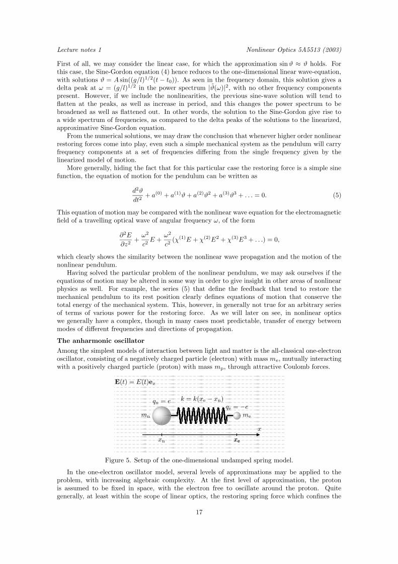
Among the simplest models of interaction between light and matter is the all-classical one-electronoscillator, consisting of a negatively charged particle (electron) with mass me, mutually interactingwith a positively charged particle (proton) with mass mp, through attractive Coulomb forces.
E(t) = E(t)ex
x
xn xe
mn
qn = e
xe
me
qe = −ek = k(xe − xn)
Figure 5. Setup of the one-dimensional undamped spring model.
In the one-electron oscillator model, several levels of approximations may be applied to theproblem, with increasing algebraic complexity. At the first level of approximation, the protonis assumed to be fixed in space, with the electron free to oscillate around the proton. Quitegenerally, at least within the scope of linear optics, the restoring spring force which confines the
17

Nonlinear Optics 5A5513 (2003) Lecture notes 1
electron can be assumed to be linear with the displacement distance of the electron from the centralposition. Providing the very basic models of the concept of refractive index and optical dispersion,this model has been applied by numerous authors, such as Feynman [R. P. Feynman, Lectureson Physics (Addison-Wesley, Massachusetts, 1963)], and Born and Wolf [M. Born and E. Wolf,Principles of Optics (Cambridge University Press, Cambridge, 1980)].
Moving on to the next level of approximation, the bound proton-electron pair may be consideredas constituting a two-body central force problem of classical mechanics, in which one may assumea fixed center of mass of the system, around which the proton as well as the electron are free tooscillate. In this level of approximation, by introducing the concept of reduced mass for the twomoving particles, the equations of motion for the two particles can be reduced to one equation ofmotion, for the evolution of the electric dipole moment of the system.
The third level of approximation which may be identified is when the center of mass is allowedto oscillate as well, in which case an equation of motion for the center of mass appears in additionto the one for the evolution of the electric dipole moment.
In each of the models, nonlinearities of the restoring central force field may be introduced as toinclude nonlinear interactions as well. It should be emphasized that the spring model, as now willbe introduced, gives an identical form of the set of nonzero elements of the susceptibility tensors,as compared with those obtained using a quantum mechanical analysis.
Throughout this analysis, the wavelength of the electromagnetic field will be assumed to besufficiently large in order to neglect any spatial variations of the fields over the spatial extent ofthe oscillator system. In this model, the central force field is modelled by a mechanical spring forcewith spring constant ke, as shown schematically in Fig. 5, and the all-classical Newton’s equationsof motion for the electron and nucleus are
me∂2xe
∂t2= −eE(t)︸ ︷︷ ︸
optical
− k0(xe − xn) + k1(xe − xn)2︸ ︷︷ ︸spring
,
mn∂2xn
∂t2= +eE(t)︸ ︷︷ ︸
optical
+ k0(xe − xn) − k1(xe − xn)2︸ ︷︷ ︸spring
,
corresponding to a system of two particles connected by a spring with spring “constant”
k = − ∂F(spring)e
∂(xe − xn)=
∂F(spring)n
∂(xe − xn)= k0 − 2k1(xe − xn).
By introducing the reduced mass12 mr = memn/(me +mn) of the system, the equation of motionfor the electric dipole moment p = −e(xe − xn) is then obtained as
∂2p
∂t2+k0
mrp+
k1
emrp2 =
e2
mrE(t). (6)
This inhomogeneous nonlinear ordinary differential equation for the electric dipole moment is theprimary interest in the discussion that now is to follow.
The electric dipole moment of the anharmonic oscillator is now expressed in terms of a pertur-bation series as
p(t) = p(0)(t) + p(1)(t)︸ ︷︷ ︸∝E(t)
+ p(2)(t)︸ ︷︷ ︸∝E2(t)
+ p(3)(t)︸ ︷︷ ︸∝E3(t)
+ . . . ,
where each term in the series is proportional to the applied electrical field strength to the poweras indicated in the superscript of repective term, and formulate the system of n + 1 equationsfor p(k), k = 0, 1, 2, . . . , n, that define the time evolution of the electric dipole. By inserting the
12 Herbert Goldstein, Classical Mechanics, 2nd ed. (Addison-Wesley, Massachusetts, 1980).
18
Lecture notes 1 Nonlinear Optics 5A5513 (2003)
perturbation series into Eq. (6), we hence have the equation
∂2p(0)
∂t2+∂2p(1)
∂t2+∂2p(2)
∂t2+∂2p(3)
∂t2+ . . .
+k0
mrp(0) +
k0
mrp(1) +
k0
mrp(2) +
k0
mrp(3) + . . .
+k1
emr(p(0) + p(1) + p(2) + . . .)(p(0) + p(1) + p(2) + . . .) =
e2
mrE(t).
Since this equation is to hold for an arbitrary electric field E(t), that is to say, at least within thelimits of the validity of the perturbation analysis, each set of terms with equal power dependenceof the electric field must individually satisfy the relation. By sorting out the various powers andidentifying terms in the left and right hand sides of the equation, we arrive at the system ofequations
∂2p(0)
∂t2+k0
mrp(0) +
k1
emrp(0)2 = 0,
∂2p(1)
∂t2+k0
mrp(1) +
k1
emr2p(0)p(1) =
e2
mrE(t),
∂2p(2)
∂t2+k0
mrp(2) +
k1
emr(2p(0)p(2) + p(1)2) = 0,
∂2p(3)
∂t2+k0
mrp(3) +
k1
emr(2p(0)p(3) + 2p(1)p(2)) = 0,
where we kept terms with powers of the electric field up to and including order three. At a firstglance, this system seem to suggest that only the first order of the perturbation series depends onthe applied electric field of the light; however, taking a closer look at the system, one can easilyverify that all orders of the dipole moment is coupled directly to the lower order terms. The systemof equations for p(k) can now be solved for k = 0, 1, 2, . . ., in that order, to successively providethe basis of solutions for higher and higher order terms, until reaching some k = n after which wemay safely neglect the reamaining terms, hence providing an approximate solution.13
The zeroth order term in the perturbation series is decribed by a nonlinear ordinary differentialequation of order two, a so-calles Riccati equation, which analytically can be solved exactly, eitherby directly applying the theory of Jacobian elliptic integrals of by applying the Riccati transor-mation.14 However, by considering a system starting from rest, at a state of equilibrium, we canimmediately draw the conclusion that p(0)(t) must be identically zero for all times t. This, ofcourse, only holds for this particular model; in many molecular systems, such in water, a perma-nent static dipole moment is present, something that is left out in this particular spring modelof ours. (Not to be confused with the static polarization induced by the electric field, which bydefinition of the terms in the perturbation series is included in higher order terms, depending onthe power of the electric field.)
The first order term in the perturbation series is the first and only one with an explicit de-pendence of the electric field of the light. Since the zeroth order perturbation term is zero, thedifferential equation for the first order term is linear, which simplifies the calculus. However, sinceit is an inhomogeneous differential equation, we must generally look for a total solution to the equa-tion as a sum of a homogeneous solution (with zero right hand side) and a particular solution (withthe electric field in the right hand side present). The homogeneous solution, which will containtwo constants of integration (since we are considering second-order ordinary differential equation)will though only give the part of the solution which depend on initial conditions, that is to say,
13 It should though be emphasized that in the limit n→ ∞, the described theory still is an exactdescription of the motion of the electric dipole moment within this model of interaction betweenlight and matter.14 For examples of the application of the Riccati transformation, see Zwillinger, Handbook ofDifferential Equations, 2nd ed. (Academic Press, Boston, 1992).
19

Nonlinear Optics 5A5513 (2003) Lecture notes 1
in this case a harmonic natural oscillation of the spring system which in the presence of dampingterms rapidly would decrease to zero. This implies that in order to find steady-state solutions, inwhich the oscillation of the dipole moment directly follows the oscillation of the electric field of thelight, we may directly start looking for the particular solution. For a time harmonic electric field,here taken as
E(t) = Eω sin(ωt),
the particular solution for the first order term is after some straightforward algebra given as15
p(1) =(e2/mr)
(k0/mr − ω2)Eω sin(ωt), ω2 6= (k0/mr).
For a material consisting of N dipoles per unit volume, and by following the conventions for thelinear electric susceptibility in SI units, this corresponds to a first order electric polarization densityof the form
P (1)(t) = P (1)ω sin(ωt)
= ε0χ(1)(ω)Eω sin(ωt),
with the first order (linear) electric susceptibility given as
χ(1)(ω) = χ(1)(−ω;ω) =N
ε0
(e2/mr)
(Ω2 − ω2),
where the resonance frequency Ω2 = k0/mr was introduced. The Lorenzian shape of the frequencydependence is shown in Fig. 6.
15 For the sake of self consistency, the general solution for the first order term is given as
p(1) = A cos((k0/mr)1/2t) +B sin((k0/mr)
1/2t) +e2/mr
k0/mr − ω2Eω sin(ωt),
where A and B are constants of integration, determined by initial conditions.
20

Lecture notes 1 Nonlinear Optics 5A5513 (2003)
0 0.5 1 1.5−10
−8
−6
−4
−2
0
2
4
6
8
10
ω/Ω
χ(1) (−
2ω;ω
,ω)
(nor
mal
ized
)
First order susceptibility
Figure 6. Lorenzian shape of the linear susceptibility χ(1)(−ω;ω).
Continuing with the second order perturbation term, some straightforward algebra gives thatthe particular solution for the second order term of the electric dipole moment becomes
p(2)(t) = − k1e3
2k0m2r
1
(Ω2 − ω2)E2ω +
k1e3
2m3r
1
(Ω2 − ω2)(Ω2 − 4ω2)E2ω
+k1e
3
m3r
1
(Ω2 − ω2)(Ω2 − 4ω2)E2ω sin2(ωt).
In terms of the polarization density of the medium, still with N dipoles per unit volume andfollowing the conventions in regular SI units, this can be written as
P (2)(t) = P(0)0 + P
(0)2ω sin(2ωt)
= ε0χ(2)(0;ω,−ω)EωEω︸ ︷︷ ︸DC polarization
+ ε0χ(2)(−2ω;ω, ω)EωEω sin(2ω)︸ ︷︷ ︸second harmonic polarization
with the second order (quadratic) electric susceptibility given as
χ(2)(0;ω,−ω) =N
ε0
k1e3
2m3r
[1
(Ω2 − ω2)(Ω2 − 4ω2)− 1
Ω2(Ω2 − ω2)
],
χ(2)(2ω;ω, ω) =N
ε0
k1e3
m3r
1
(Ω2 − ω2)(Ω2 − 4ω2).
From this we may notice that for one-photon resonances, the nonlinearities are enhanced wheneverω ≈ Ω or 2ω ≈ Ω, for the induced DC as well as the second harmonic polarization density.
The explicit frequency dependencies of the susceptibilities χ(2)(−2ω;ω, ω) and χ(2)(0;ω,−ω)are shown in Figs. 7 and 8.
21

Nonlinear Optics 5A5513 (2003) Lecture notes 1
0 0.5 1 1.5−10
−8
−6
−4
−2
0
2
4
6
8
10
ω/Ω
χ(2) (−
2ω;ω
,ω)
(nor
mal
ized
)
Second order susceptibility (SHG)
Figure 7. Lorenzian shape of the linear susceptibility χ(2)(−2ω;ω, ω) (SHG).
0 0.5 1 1.5−10
−8
−6
−4
−2
0
2
4
6
8
10
ω/Ω
χ(2) (0
;ω,−
ω)
(nor
mal
ized
)
Second order susceptibility (DC rectification)
Figure 8. Lorenzian shape of the linear susceptibility χ(2)(0;ω,−ω) (DC).
A well known fact in electromagnetic theory is that an electric dipole that oscillates at a certainangular frequency, say at 2ω, also emits electromagnetic radiation at this frequency. In particular,this implies that the term described by the susceptibility χ(2)(−2ω;ω, ω) will generate light attwice the angular frequency of the light, hence generating a second harmonic light wave.
22
Lecture Notes on Nonlinear Optics Nonlinear Optics 5A5513 (2003)
Lecture II
23

Nonlinear Optics 5A5513 (2003) Lecture Notes on Nonlinear Optics
Lecture Notes on Nonlinear OpticsNonlinear Optics (5A5513, 5p for advanced undergraduate and doctoral students)Course given at the Royal Institute of Technology,Department of Laser Physics and Quantum OpticsSE–106 91, Stockholm, SwedenJanuary 8 – March 24, 2003
The texts and figures in this lecture series was typeset by the author in 10/12/16 pt ComputerModern typeface using plain TEX and METAPOST.
This document is electronically available at the homepage of the Library of the Royal Institute ofTechnology, at http://www.lib.kth.se.
Copyright c© Fredrik Jonsson 2003
All rights reserved. No part of this publication may be reproduced, stored in a retrieval system,or transmitted, in any form, or by any means, electronic, mechanical, photo-copying, recording, orotherwise, without the prior consent of the author.
ISBN 91-7283-517-6TRITA-FYS 2003:26ISSN 0280-316XISRN KTH/FYS/- - 03:26 - - SEPrinted on July 7, 2003
TEX is a trademark of the American Mathematical Society
24

Nonlinear Optics 5A5513 (2003)Lecture notes
Lecture 2
Nonlinear polarization density
From the introductory perturbation analysis of the all-classical anharmonic oscillator in the pre-vious lecture, we now a priori know that it is possible to express the electric polarization densityas a power series in the electric field of the optical wave.
Loosely formulated, the electric polarization density in complex notation can be taken as theseries
Pµ(ωσ) = ε0[χ(1)µα(−ωσ;ωσ)Eα(ωσ)︸ ︷︷ ︸
∼P(1)µ (ωσ)
+ χ(2)µαβ(−ωσ;ω1, ω2)Eα(ω1)Eβ(ω2)︸ ︷︷ ︸
∼P(2)µ (ωσ), ωσ=ω1+ω2
+ χ(3)µαβγ(−ωσ;ω1, ω2, ω3)Eα(ω1)Eβ(ω2)Eγ(ω3)︸ ︷︷ ︸
∼P(3)µ (ωσ), ωσ=ω1+ω2+ω3
+ . . . ]
where we adopted Einstein’s convention of summation for terms with repeated subscripts. (A moreformal formulation of the polarization density will be described later.)
Symmetries in nonlinear optics
There are essentially four classes of symmetries that we will encounter in this course:
[1] Intrinsic permutation symmetry:
χ(3)µαβγ(−ωσ;ω1, ω2, ω3) = χ
(3)µβαγ(−ωσ;ω2, ω1, ω3)
= χ(3)µβγα(−ωσ;ω2, ω3, ω1)
= χ(3)µγβα(−ωσ;ω3, ω2, ω1),
that is to say, invariance under the n! possible permutations of (αk, ωk), k = 1, 2, . . . , n. Thisprinciple applies generally to resonant as well as nonresonant media. (Described in this lecture.)
[2] Overall permutation symmetry:
χ(3)µαβγ(−ωσ;ω1, ω2, ω3) = χ
(3)αµβγ(ω1;−ωσ, ω2, ω3)
= χ(3)αβµγ(ω1;ω2,−ωσ, ω3)
= χ(3)αβγµ(ω1;ω2, ω3,−ωσ),
that is to say, invariance under the (n + 1)! possible permutations of (µ,−ωσ), (αk, ωk), k =1, 2, . . . , n. This principle applies to nonresonant media, where all optical frequencies appearingin the formula for the susceptibility are removed far from the transition frequencies of themedium. (Described in lecture 4.)
[3] Kleinman symmetry:
χ(3)µαβγ(−ωσ;ω1, ω2, ω3) = χ
(3)αµβγ(−ωσ;ω1, ω2, ω3)
= χ(3)αβµγ(−ωσ;ω1, ω2, ω3)
= χ(3)αβγµ(−ωσ;ω1, ω2, ω3),
25

Nonlinear Optics 5A5513 (2003) Lecture notes 2
that is to say, invariance under the (n+1)! possible permutations of the subscripts µ, α1, . . . , αn.This principle is a consequence of the overall permutation symmetry, and applies in the low-frequency limit of nonresonant media.
[4] Spatial symmetries, given by the point symmetry class of the medium. (Described in lecture 6.)
Conditions for observing nonlinear optical interactions
Loosely formulated, a nonlinear response between light and matter depends on one of two keyindgredients: either there is a resonance between the light wave and some natural oscillation modeof the medium, or the light is sufficiently intense. Direct resonance can occur in isolated intervalsof the electromagnetic spectrum at• ultraviolet and visible frequencies (1015 s−1) where the oscillator corresponds to an electronic
transition of the medium,• infrared (1013 s−1), where the medium has vibrational modes, and• the far infrared-microwave range (1011 s−1), where there are rotational modes. These interac-
tions are also called one-photon processes, and are schematically illustrated in Fig. 3.
|a〉
|b〉
hω hω
The one-photon transition.
Figure 3. Transition scheme of the one-photon process.
The lower frequency modes can be excited at optical frequencies (1015 s−1) through indirect reso-nant processes in which the difference in frequencies and wave vectors of two light waves, called thepump and Stokes wave, respectively, matches the frequency and wave vector of one of these lowerfrequency modes. These three-frequency interactions are sometime called two-photon processes.In the case where there “lower frequency” mode is an electronic transition or in the vibrationalrange (in which case the Stokes frequency can be of the same order of magnitude as that of thelight wave), this process is called Raman scattering.
|a〉 (initial)
|c〉 (final)
|b〉
hω1 hω2
The Stokes Raman transition.
|a〉 (final)
|c〉 (initial)
|b〉
hω1 hω2
The Anti-Stokes Raman transition.
Figure 4. Transition schemes of stimulated Raman Scattering.
The stimulated Raman scattering is essentially a two-photon process in which one photon at ω1
is absorbed and one photon at ω2 is emitted, while the material makes a transition from theinitial state |a〉 to the final state |c〉, as shown in Fig. 4. Energy conservation requires the Ramanresonance frequency (electronic or vibrational) to satisfy ~Ωca = ~(ω1 − ω2), and hence we may
26

Lecture notes 2 Nonlinear Optics 5A5513 (2003)
classify the Stokes and Anti-Stokes transitions as
~Ωca > 0 ⇔ Stokes Raman
~Ωca < 0 ⇔ Anti − Stokes Raman
When the lower frequency mode instead is an acoustic mode of the material, the process is insteadcalled Brillouin scattering.
As will be shown explicitly later on in the course, optical resonance with transitions of thematerial is an important tool for “boosting up” the nonlinearities, with enhanced possibilities ofapplications. However, at single-photon resonance we have a strong absorption at the frequencyof the optical field, and in most cases this is a non-desirable effect, since it decreases the opticalintensity, even though it meanwhile also enhances the nonlinearity of the material.
However, by instead exploiting the two-photon resonance, the desired nonlinearity can be sig-nificantly enhanced whilst at the same time the competing absorption process can be minimizedby avoiding coincidences between optical frequencies and single-photon resonances.
One general drawback with the resonant enhancement is that the response time of the polar-ization density of the material is slowed down, affecting applications such as optical switching ormodulation, where speed is of importance.
Phenomenological description of the susceptibility tensors
Before entering the full quantum-mechanical formalism, we will assume the medium to possess atemporal response described by time response functions R(t).
The very first step in the analysis is to express the electric polarization density, which in classicalelectrodynamical terms is expressed as the sum over all M electric charges qk in a small volume Vcentered at r,
P(r, t) =1
V
M∑
k=1
qkrk(t),
as a series expansion
P(r, t) = P(0)(r, t) + P(1)(r, t) + P(2)(r, t) + . . .+ P(n)(r, t) + . . . ,
where P(1)(r, t) is linear in the electric field, P(2)(r, t) is quadratic in the electric field, etc. Thefield-independent P(0)(r, t) corresponds to eventually appearing static polarization of the medium.It should be emphasized that any of these terms may be linear as well as nonlinear functions ofthe electric field of the optical wave; i. e. an externally applied static electric field may togetherwith the electric field of the light interact through, for example, P(3)(r, t) to induce an electricpolarization that is linear in the optical field.
R(t− τ)
tt = τ
R = 0
Figure 9. Schematic form of a possible response function in time domain.
In the analysis that now is to follow, we will a priori assume that it is possible to express thepolarization density as a perturbation series. Later on, we will show how each of the terms can bederived from a more stringent basis, where it also will be stated which conditions that must holdin order to apply perturbation theory.
27

Nonlinear Optics 5A5513 (2003) Lecture notes 2
Linear polarization response function
Since P(1)(r, t) is taken as linear in the electric field, we may express the linear polarization densityof the medium as being related to the optical field as
P (1)µ (r, t) = ε0
∫ ∞
−∞
T (1)µα (t; τ)Eα(r, τ) dτ, (7)
where T(1)µα (t; τ) is a rank-two tensor that weights all contributions in time from the electric field
of the light. A few required properties of T(1)µα (t; τ) can immediately be stated:
• Causality. We require that no optically induced contribution can occur before the field is
applied, i. e. T(1)µα (t; τ) = 0 for t ≤ τ .
• Time invariance. Under most circumstances, we may in addition assume that the material
parameters are constant in time, such that P(1)µ (r, t′) is identical to the polarisation as induced
by the time-displaced electric field Eα(r, t′).
The second of these properties is essentially a manifestation of an adiabatically following changeof the carrier wave of the optical field.
By using Eq. (7), the time invariance of the constitutive relation gives that
P (1)µ (r, t+ t0) = ε0
∫ ∞
−∞
T (1)µα (t+ t0; τ)Eα(r, τ) dτ
=Should equal to polarization induced by Eα(r, τ + t0)
= ε0
∫ ∞
−∞
T (1)µα (t; τ)Eα(r, τ + t0) dτ
=τ ′ = τ + t0
= ε0
∫ ∞
−∞
T (1)µα (t; τ ′ − t0)Eα(r, τ ′) dτ ′,
from which we, by changing the “dummy” variable of integration back to τ , obtain the relation
T (1)µα (t+ t0; τ) = T (1)
µα (t; τ − t0).
In particular, by setting t = 0 and replacing the arbitrary time displacement t0 by t, one finds thatthe response of the medium depends only of the time difference τ − t,
T (1)µα (t; τ) = T (1)
µα (0; τ − t)
= R(1)µα(τ − t)
where we defined the linear polarization response function R(1)µα(τ − t), being a rank-two tensor
depending only on the time difference τ − t.To summarize, the linear contribution to the electric polarization density is given in terms of
the linear polarization response function as
P (1)µ (r, t) = ε0
∫ ∞
−∞
R(1)µα(t− τ)Eα(r, τ) dτ,
= ε0
∫ ∞
−∞
R(1)µα(τ ′)Eα(r, t− τ ′) dτ ′,
(8)
and the causality condition for the linear polarization response function requires that
R(1)µα(τ − t) = 0, t ≤ τ,
and in addition, since the relation (8) is to hold for arbitrary time evolution of the electrical field,
and since the polarization density P(1)µ (r, t) and the electric field E
(1)α (r, t) both are real-valued
quantities, we also require the polarization response function R(1)µα(τ−t) to be a real-valued function.
28

Lecture notes 2 Nonlinear Optics 5A5513 (2003)
Quadratic polarization response function
The second-order, quadratic polarization density can in similar to the linear one be phenomeno-logically be written as the sum of all infinitesimal previous contributions in time. In this case,we must though include the possibility that not all contributions origin in the same time scale,and hence the proper formulation of the second order polarization density is as a two-dimensionalintegral,
P (2)µ (r, t) = ε0
∫ ∞
−∞
∫ ∞
−∞
T(2)µαβ(t; τ1, τ2)Eα(r, τ1)Eβ(r, τ2) dτ1 dτ2. (9)
The tensor T(2)µαβ(t; τ1, τ2) uniquely determines the quadratic, second-order polarization of the
medium. However, the tensor T(2)µαβ(t; τ1, τ2) is not itself unique. To see this, we may express
the tensor as a sum of a symmetric part and an antisymmetric part,
T(2)µαβ(t; τ1, τ2) =
1
2
[T
(2)µαβ(t; τ1, τ2) + T
(2)µβα(t; τ2, τ1)
]
︸ ︷︷ ︸symmetric
+1
2
[T
(2)µαβ(t; τ1, τ2) − T
(2)µβα(t; τ2, τ1)
]
︸ ︷︷ ︸antisymmetric
= S(2)µαβ(t; τ1, τ2)︸ ︷︷ ︸
=S(2)
µβα(t;τ2,τ1)
+A(2)µαβ(t; τ1, τ2)︸ ︷︷ ︸
=−A(2)
µβα(t;τ2,τ1)
As this form of the response function is inserted into the original expression (9) for the secondorder polarization density, we immediately find that it is left invariant under the interchange of thedummy variables (α, τ1) and (β, τ2) (since the integration is performed from minus to plus infinityin time). In particular, it from this follows that
P (2)µ (r, t) = ε0
∫ ∞
−∞
∫ ∞
−∞
[S(2)µαβ(t; τ1, τ2) +A
(2)µαβ(t; τ1, τ2)]Eα(r, τ1)Eβ(r, τ2) dτ1 dτ2
= ε0
∫ ∞
−∞
∫ ∞
−∞
S(2)µαβ(t; τ1, τ2)Eα(r, τ1)Eβ(r, τ2) dτ1 dτ2
︸ ︷︷ ︸≡I1
+ ε0
∫ ∞
−∞
∫ ∞
−∞
A(2)µαβ(t; τ1, τ2)Eα(r, τ1)Eβ(r, τ2) dτ1 dτ2
︸ ︷︷ ︸≡I2
= ε0
∫ ∞
−∞
∫ ∞
−∞
S(2)µβα(t; τ2, τ1)Eα(r, τ1)Eβ(r, τ2) dτ1 dτ2
− ε0
∫ ∞
−∞
∫ ∞
−∞
A(2)µβα(t; τ2, τ1)Eα(r, τ1)Eβ(r, τ2) dτ1 dτ2
= ε0
∫ ∞
−∞
∫ ∞
−∞
S(2)µβα(t; τ2, τ1)Eβ(r, τ2)Eα(r, τ1) dτ1 dτ2
︸ ︷︷ ︸=I1
− ε0
∫ ∞
−∞
∫ ∞
−∞
A(2)µβα(t; τ2, τ1)Eβ(r, τ2)Eα(r, τ1) dτ1 dτ2
︸ ︷︷ ︸=I2
i. e. the symmetric part satisfy the trivial identity I1 = I1, while the antisymmetric part satisfyI2 = −I2, i. e. the antisymmetric part does not contribute to the polarization density, and thatwe may set the antiymmetric part to zero, without imposing any constraint on the validity of thetheory.
The time response T(2)µαβ(t; τ1, τ2) is then unique and now chosen to be symmetric,
T(2)µαβ(t; τ1, τ2) = T
(2)µβα(t; τ2, τ1).
29

Nonlinear Optics 5A5513 (2003) Lecture notes 2
This procedure of symmetrization may seem like an all theoretical contruction, somewhat out offocus of what lies ahead, but in fact it turns out to be an extremely useful property that welater on will exploit extensively. The previously described symmetric property will later on, forsusceptibility tensors in the frequency domain, be denoted as the intrinsic permutation symmetry,a general property that will hold irregardless of whether the nonlinear interaction under analysisis highly resonant or far from resonance.
By again applying the arguments of time invariance, as previously for the linear responsefunction, we find that
T(2)µαβ(t+ t0; τ1, τ2) = T
(2)µαβ(t; τ1 − t0, τ2 − t0)
for all t, τ1, and τ2. Hence, by setting t = 0 and then replacing th arbitrary time t0 by t, againas previously done for the linear case, one finds that T (2)(t; τ1, τ2) depends only on the two timedifferences t− τ1 and t− τ2. To make this fact explicit, we may hence write the response functionas
T(2)µαβ(t; τ1, τ2) = R
(2)µαβ(t− τ1, t− τ2),
giving the canonical form of the quadratic polarization density as
P (2)µ (r, t) = ε0
∫ ∞
−∞
∫ ∞
−∞
R(2)µαβ(t− τ1, t− τ2)Eα(r, τ1)Eβ(r, τ2) dτ1 dτ2
= ε0
∫ ∞
−∞
∫ ∞
−∞
R(2)µαβ(τ
′1, τ
′2)Eα(r, t− τ ′1)Eβ(r, t− τ ′2) dτ
′1 dτ
′2.
(10)
The tensor R(2)µαβ(τ1, τ2) is called the quadratic electric polarization response of the medium, and in
similar with the linear response function, arguments of causality require the response function tobe zero whenever τ1 and/or τ2 is negative. Similarly, the reality condition on Eα(r, t) and Pα(r, t)
requires that R(2)µαβ(τ1, τ2) is a real-valued function.
Higher order polarization response functions
The nth order polarization density can in similar to the linear (n = 1 and quadratic (n = 2) onesbe written as
P (n)µ (r, t) = ε0
∫ ∞
−∞
· · ·∫ ∞
−∞
R(n)µα1···αn
(t− τ1, . . . , t− τn)Eα1(r, τ1) · · ·Eαn
(r, τn) dτ1 · · · dτn
= ε0
∫ ∞
−∞
· · ·∫ ∞
−∞
R(n)µα1···αn
(τ ′1, . . . , τ′n)Eα1
(r, t− τ ′1) · · ·Eαn(r, t− τ ′n) dτ
′1 · · · dτ ′n,
(11)
where the nth order response function is a tensor of rank n + 1, and a real-valued function ofthe n parameters τ1, . . . , τn, vanishing whenever any τk < 0, k = 1, 2, . . . , n, and with the intrin-sic permutation symmetry that it is left invariant under any of the n! pairwise permutations of(α1, τ1), . . . , (αn, τn).
30

Lecture Notes on Nonlinear Optics Nonlinear Optics 5A5513 (2003)
Lecture III
31

Nonlinear Optics 5A5513 (2003) Lecture Notes on Nonlinear Optics
Lecture Notes on Nonlinear OpticsNonlinear Optics (5A5513, 5p for advanced undergraduate and doctoral students)Course given at the Royal Institute of Technology,Department of Laser Physics and Quantum OpticsSE–106 91, Stockholm, SwedenJanuary 8 – March 24, 2003
The texts and figures in this lecture series was typeset by the author in 10/12/16 pt ComputerModern typeface using plain TEX and METAPOST.
This document is electronically available at the homepage of the Library of the Royal Institute ofTechnology, at http://www.lib.kth.se.
Copyright c© Fredrik Jonsson 2003
All rights reserved. No part of this publication may be reproduced, stored in a retrieval system,or transmitted, in any form, or by any means, electronic, mechanical, photo-copying, recording, orotherwise, without the prior consent of the author.
ISBN 91-7283-517-6TRITA-FYS 2003:26ISSN 0280-316XISRN KTH/FYS/- - 03:26 - - SEPrinted on July 7, 2003
TEX is a trademark of the American Mathematical Society
32
Nonlinear Optics 5A5513 (2003)Lecture notes
Lecture 3
Susceptibility tensors in the frequency domain
The susceptibility tensors in the frequency domain arise when the electric field Eα(t) of the lightis expressed in terms of its Fourier transform Eα(ω), by means of the Fourier integral identity
Eα(t) =
∫ ∞
−∞
Eα(ω) exp(−iωt) dω = F−1[Eα](t), (1′)
with inverse relation
Eα(ω) =1
2π
∫ ∞
−∞
Eα(τ) exp(iωτ) dτ = F[Eα](ω). (1′′)
This convention of inclusion of the factor of 2π, as well as the sign convention, is commonly usedin quantum mechanics; however, it should be emphasized that this convention is not a commonlyadopted standard in optics, neither in linear nor in nonlinear optical regimes.
The sign convention here used leads to wave solutions of the form f(kz−ωt) for monochromaticwaves propagating in the positive z-direction, which might be somewhat more intuitive than thealternative form f(ωt−kz), which is obtained if one instead apply the alternative sign convention.
The convention for the inclusion of 2π in the Fourier transform in Eq. (1′′) is here convenientfor description of electromagnetic wave propagation in the frequency domain (going from the timedomain description, in terms of the polarization response functions, to the frequency domain, interms of the linear and nonlinear susceptibilities), since it enables us to omit any multiple of 2π ofthe Fourier transformed fields.
First order susceptibility tensor
By inserting Eq. (1′) is inserted into the previously obtained1 relation for the first order, linearpolarization density, one obtains
P (1)µ (r, t) = ε0
∫ ∞
−∞
R(1)µα(τ)Eα(r, t− τ) dτ,
= express Eα(r, t− τ) in frequency domain
= ε0
∫ ∞
−∞
R(1)µα(τ)
∫ ∞
−∞
Eα(r, ω) exp[−iω(t− τ)] dω dτ,
= change order of integration
= ε0
∫ ∞
−∞
∫ ∞
−∞
R(1)µα(τ)Eα(r, ω) exp(iωτ) dτ exp(−iωt) dω,
= ε0
∫ ∞
−∞
χ(1)µα(−ω;ω)Eα(r, ω) exp(−iωt) dω,
(2)
where the linear electric dipolar susceptibility,
χ(1)µα(−ω;ω) =
∫ ∞
−∞
R(1)µα(τ) exp(iωτ) dτ = F[R(1)
µα](ω), (3)
1 Expressions for the first order, second order, and nth order polarization densities were obtainedin lecture two.
33

Nonlinear Optics 5A5513 (2003) Lecture notes 3
was introduced. In this expression for the susceptibility, ωσ = ω, and the reasons for the somewhatpeculiar notation of arguments of the susceptibility will be explained later on in the context ofnonlinear susceptibilities.
Second order susceptibility tensor
In similar to the linear susceptibility tensor, by inserting Eq. (1′) into the previously obtainedrelation for the second order, quadratic polarization density, one obtains
P (2)µ (r, t) = ε0
∫ ∞
−∞
∫ ∞
−∞
∫ ∞
−∞
∫ ∞
−∞
R(2)µαβ(τ1, τ2)Eα(r, ω1)Eβ(r, ω2)
× exp[−i(ω1(t− τ1) + ω2(t− τ2))] dτ1 dτ2 dω1 dω2
= ε0
∫ ∞
−∞
∫ ∞
−∞
χ(2)µαβ(−ωσ;ω1, ω2)Eα(r, ω1)Eβ(r, ω2) exp[−i (ω1 + ω2)︸ ︷︷ ︸
≡ωσ
t] dω1 dω2
(4)
where the quadratic electric dipolar susceptibility,
χ(2)µαβ(−ωσ;ω1, ω2) =
∫ ∞
−∞
∫ ∞
−∞
R(2)µαβ(τ1, τ2) exp[i(ω1τ1 + ω2τ2)] dτ1 dτ2, (5)
was introduced. In this expression for the susceptibility, ωσ = ω1 + ω2, and the reason for thenotation of arguments should now be somewhat more clear: the first angular frequency argumentof the susceptibility tensor is simply the sum of all driving angular frequencies of the optical field.
The intrinsic permutation symmetry of R(2)µαβ(τ1, τ2), the second order polarization response
function, carries over to the second order susceptibility tensor as well, in the sense that
χ(2)µαβ(−ωσ;ω1, ω2) = χ
(2)µβα(−ωσ;ω2, ω1),
i. e. the second order susceptibility is invariant under any of the 2! = 2 pairwise permutations of(α, ω1) and (β, ω2).
Higher order susceptibility tensors
In similar to the linear and quadratic susceptibility tensors, by inserting Eq. (1′) into the previouslyobtained relation for the nth order polarization density, one obtains
P (n)µ (r, t) = ε0
∫ ∞
−∞
· · ·∫ ∞
−∞
χ(n)µα1···αn
(−ωσ;ω1, . . . , ωn)Eα1(r, ω1) · · ·Eαn
(r, ωn)
× exp[−i (ω1 + . . .+ ωn)︸ ︷︷ ︸≡ωσ
t] dω1 · · · dωn,(6)
where the nth order electric dipolar susceptibility,
χ(n)µα1···αn
(−ωσ;ω1, . . . , ωn) =
∫ ∞
−∞
· · ·∫ ∞
−∞
R(n)µα1···αn
(τ1, . . . , τn) exp[i(ω1τ1+. . .+ωnτn)] dτ1 · · · dτn,(7)
was introduced, and where, as previously,
ωσ = ω1 + ω2 + . . .+ ωn.
The intrinsic permutation symmetry of R(n)µα1···αn
(τ1, . . . , τn), the nth order polarization re-sponse function, also in this general case carries over to the nth order susceptibility tensor as well,in the sense that
χ(n)µα1α2···αn
(−ωσ;ω1, ω2, . . . , ωn)
is invariant under any of the n! pairwise permutations of (α1, ω1), (α2, ω2), . . ., (αn, ωn).
34

Lecture notes 3 Nonlinear Optics 5A5513 (2003)
Monochromatic fields
It should at this stage be emphasized that even though the electric field via the Fourier integralidentity can be seen as a superposition of infinitely many infinitesimally narrow band monochro-matic components, the superposition principle of linear optics, which states that the wave equationmay be independently solved for each frequency component of the light, generally does not holdin nonlinear optics.
For monochromatic light, the electric field can be written as a superposition of a set of distinctterms in time domain as
E(r, t) =∑
k
Re[Eωkexp(−iωkt)],
with the convention that the involved angular frequencies all are taken as positive, ωk ≥ 0, andthe electric field in the frequency domain simply becomes a superposition of delta peaks in thespectrum,
E(r, ω) =1
2π
∫ ∞
−∞
E(r, τ) exp(iωτ) dτ
= express as monochromatic field
=1
2π
∑
k
∫ ∞
−∞
Re[Eωkexp(−iωkτ)] exp(iωτ) dτ
= by definition
=1
4π
∑
k
∫ ∞
−∞
[Eωkexp(i(ω − ωk)τ) + E∗
ωkexp(i(ω + ωk)τ)] dτ
=1
2
∑
k
[Eωk
1
2π
∫ ∞
−∞
exp(i(ω − ωk)τ) dτ
︸ ︷︷ ︸≡δ(ω−ωk)
+E∗ωk
1
2π
∫ ∞
−∞
exp(i(ω + ωk)τ) dτ
︸ ︷︷ ︸≡δ(ω+ωk)
]
= definition of the delta function
=1
2
∑
k
[Eωkδ(ω − ωk) + E∗
ωkδ(ω + ωk)].
By inserting this form of the electric field (taken in the frequency domain) into the polarizationdensity, one obtains the polarization density in the monochromatic form
P(n)(r, t) =∑
ωσ≥0
Re[P(n)ωσ
exp(−iωσt)],
with complex-valued Cartesian components at angular frequency ωσ given as
(P(n)ωσ
)µ = 2ε0∑
α1
· · ·∑
αn
χ(n)µα1α2···αn
(−ωσ;ω1, ω2, . . . , ωn)(Eω1)α1
(Eω2)α2
· · · (Eωn)αn
+ χ(n)µα1α2···αn
(−ωσ;ω2, ω1, . . . , ωn)(Eω2)α1
(Eω1)α2
· · · (Eωn)αn
+ all other distinguishable terms
(8)
where, as previously, ωσ = ω1 + ω2 + . . . + ωn. In the right hand side of Eq. (8), the summationis performed over all distinguishble terms, that is to say over all the possible combinations ofω1, ω2, . . . , ωn that give rise to the particular ωσ. Within this respect, a certain frequency andits negative counterpart are to be considered as distinct frequencies when appearing in the set.In general, there are several possible combinations that give rise to a certain ωσ; for example(ω, ω,−ω), (ω,−ω, ω), and (−ω, ω, ω) form the set of distinct combinations of optical frequenciesthat give rise to optical Kerr-effect (a field dependent contribution to the polarization density atωσ = ω + ω − ω = ω).
A general conclusion of the form of Eq. (8), keeping the intrinsic permutation symmetry inmind, is that only one term needs to be written, and the number of times this term appearsin the expression for the polarization density should consequently be equal to the number ofdistinguishable combinations of ω1, ω2, . . . , ωn.
35

Nonlinear Optics 5A5513 (2003) Lecture notes 3
Convention for description of nonlinear optical polarization
As a “recipe” in theoretical nonlinear optics, Butcher and Cotter provide a very useful conventionwhich is well worth to hold on to. For a superposition of monochromatic waves, and by invokingthe general property of the intrinsic permutation symmetry, the monochromatic form of the nthorder polarization density can be written as
(P (n)ωσ
)µ = ε0∑
α1
· · ·∑
αn
∑
ω
K(−ωσ;ω1, . . . , ωn)χ(n)µα1···αn
(−ωσ;ω1, . . . , ωn)(Eω1)α1
· · · (Eωn)αn
.
(9)The first summations in Eq. (9), over α1, . . . , αn, is simply an explicit way of stating that theEinstein convention of summation over repeated indices holds. The summation sign
∑ω, however,
serves as a reminder that the expression that follows is to be summed over all distinct sets ofω1, . . . , ωn. Because of the intrinsic permutation symmetry, the frequency arguments appearing inEq. (9) may be written in arbitrary order.
By “all distinct sets of ω1, . . . , ωn”, we here mean that the summation is to be performed, asfor example in the case of optical Kerr-effect, over the single set of nonlinear susceptibilities thatcontribute to a certain angular frequency as (−ω;ω, ω,−ω) or (−ω;ω,−ω, ω) or (−ω;−ω, ω, ω).In this example, each of the combinations are considered as distinct, and it is left as an arbitarychoice which one of these sets that are most convenient to use (this is simply a matter of choosingnotation, and does not by any means change the description of the interaction).
In Eq. (9), the degeneracy factor K is formally described as
K(−ωσ;ω1, . . . , ωn) = 2l+m−np
wherep = the number of distinct permutations of ω1, ω2, . . . , ω1,
n = the order of the nonlinearity,
m = the number of angular frequencies ωk that are zero, and
l =
1, if ωσ 6= 0,0, otherwise.
In other words, m is the number of DC electric fields present, and l = 0 if the nonlinearity we areanalyzing gives a static, DC, polarization density, such as in the previously (in the spring model)described case of optical rectification in the presence of second harmonic fields (SHG).
A list of frequently encountered nonlinear phenomena in nonlinear optics, including the degen-eracy factors as conforming to the above convention, is given in Butcher and Cotters book, Table2.1, on page 26.
Note on the complex representation of the optical field
Since the observable electric field of the light, in Butcher and Cotters notation taken as
E(r, t) =1
2
∑
ωk≥0
[Eωkexp(−iωkt) + E∗
ωkexp(iωkt)],
is a real-valued quantity, it follows that negative frequencies in the complex notation should beinterpreted as the complex conjugate of the respective field component, or
E−ωk= E∗
ωk.
Example: Optical Kerr-effect
Assume a monochromatic optical wave (containing forward and/or backward propagating compo-nents) polarized in the xy-plane,
E(z, t) = Re[Eω(z) exp(−iωt)] ∈ R3,
36

Lecture notes 3 Nonlinear Optics 5A5513 (2003)
with all spatial variation of the field contained in
Eω(z) = exExω(z) + eyE
yω(z) ∈ C
3.
Optical Kerr-effect is in isotropic media described by the third order susceptibility
χ(3)µαβγ(−ω;ω, ω,−ω),
with nonzero components of interest for the xy-polarized beam given in Appendix 3.3 of Butcherand Cotters book as
χ(3)xxxx = χ(3)
yyyy , χ(3)xxyy = χ(3)
yyxx =
intr. perm. symm.
(α, ω) (β, ω)
= χ(3)
xyxy = χ(3)yxyx, χ(3)
xyyx = χ(3)yxxy ,
withχ(3)xxxx = χ(3)
xxyy + χ(3)xyxy + χ(3)
xyyx.
The degeneracy factor K(−ω;ω, ω,−ω) is calculated as
K(−ω;ω, ω,−ω) = 2l+m−np = 21+0−33 = 3/4.
From this set of nonzero susceptibilities, and using the calculated value of the degeneracy factor inthe convention of Butcher and Cotter, we hence have the third order electric polarization density
at ωσ = ω given as P(n)(r, t) = Re[P(n)ω exp(−iωt)], with
P(3)ω =
∑
µ
eµ(P(3)ω )µ
= Using the convention of Butcher and Cotter
=∑
µ
eµ
[ε0
3
4
∑
α
∑
β
∑
γ
χ(3)µαβγ(−ω;ω, ω,−ω)(Eω)α(Eω)β(E−ω)γ
]
= Evaluate the sums over (x, y, z) for field polarized in the xy plane
= ε03
4ex[χ(3)
xxxxExωE
xωE
x−ω + χ(3)
xyyxEyωE
yωE
x−ω + χ(3)
xyxyEyωE
xωE
y−ω + χ(3)
xxyyExωE
yωE
y−ω]
+ ey[χ(3)yyyyE
yωE
yωE
y−ω + χ(3)
yxxyExωE
xωE
y−ω + χ(3)
yxyxExωE
yωE
x−ω + χ(3)
yyxxEyωE
xωE
x−ω]
= Make use of E−ω = E∗ω and relations χ(3)
xxyy = χ(3)yyxx, etc.
= ε03
4ex[χ(3)
xxxxExω|Exω|2 + χ(3)
xyyxEyω
2Ex∗ω + χ(3)xyxy |Eyω|2Exω + χ(3)
xxyyExω|Eyω|2]
+ ey[χ(3)xxxxE
yω|Eyω|2 + χ(3)
xyyxExω
2Ey∗ω + χ(3)xyxy |Exω|2Eyω + χ(3)
xxyyEyω|Exω|2]
= Make use of intrinsic permutation symmetry
= ε03
4ex[(χ(3)
xxxx|Exω|2 + 2χ(3)xxyy |Eyω|2)Exω + (χ(3)
xxxx − 2χ(3)xxyy)E
yω
2Ex∗ω
ey[(χ(3)xxxx|Eyω|2 + 2χ(3)
xxyy |Exω|2)Eyω + (χ(3)xxxx − 2χ(3)
xxyy)Exω
2Ey∗ω .
For the optical field being linearly polarized, say in the x-direction, the expression for the polar-ization density is significantly simplified, to yield
P(3)ω = ε0(3/4)exχ
(3)xxxx|Exω|2Exω,
i. e. taking a form that can be interpreted as an intensity-dependent (∼ |Exω|2) contribution to the
refractive index (cf. Butcher and Cotter §6.3.1).
37

Nonlinear Optics 5A5513 (2003) Lecture notes 3
38

Lecture Notes on Nonlinear Optics Nonlinear Optics 5A5513 (2003)
Lecture IV
39

Nonlinear Optics 5A5513 (2003) Lecture Notes on Nonlinear Optics
Lecture Notes on Nonlinear OpticsNonlinear Optics (5A5513, 5p for advanced undergraduate and doctoral students)Course given at the Royal Institute of Technology,Department of Laser Physics and Quantum OpticsSE–106 91, Stockholm, SwedenJanuary 8 – March 24, 2003
The texts and figures in this lecture series was typeset by the author in 10/12/16 pt ComputerModern typeface using plain TEX and METAPOST.
This document is electronically available at the homepage of the Library of the Royal Institute ofTechnology, at http://www.lib.kth.se.
Copyright c© Fredrik Jonsson 2003
All rights reserved. No part of this publication may be reproduced, stored in a retrieval system,or transmitted, in any form, or by any means, electronic, mechanical, photo-copying, recording, orotherwise, without the prior consent of the author.
ISBN 91-7283-517-6TRITA-FYS 2003:26ISSN 0280-316XISRN KTH/FYS/- - 03:26 - - SEPrinted on July 7, 2003
TEX is a trademark of the American Mathematical Society
40

Nonlinear Optics 5A5513 (2003)Lecture notes
Lecture 4
The Truth of polarization densitites
So far, we have performed the analysis in a theoretical framework that has been exclusively formu-lated in terms of phenomenological models, such as the anharmonic oscillator and the phenomeno-logically introduced polarization response function of the medium. In the real world applicationof nonlinear optics, however, we should not restrict the theory just to phenomenological models,but rather take advantage over the full quantum-mechanical framework of analysis of interactionbetween light and matter.
y
z
x
V
r
rk,+Zke
rj ,−e
Figure 1. Schematic figure of the ensemble in the “small volume”.
In a small volume V (smaller than the wavelength of the light, to ensure that the natural spatialvariation of the light is not taken into account, but large enough in order to contain a sufficcientnumber of molecules in order to ignore the quantum-mechanical fluctuations of the dipole momentdensity), we consider the applied electric field to be homogeneous, and the electric polarizationdensity of the medium is then given as the expectation value of the electric dipole operator of theensemble of molecules divided by the volume, as
Pµ(r, t) = 〈Qµ〉/V ,
where the electric dipole operator of the ensemble contained in V can be written as a sum over allelectrons and nuclei as
Q = −e∑
j
rj
︸ ︷︷ ︸electrons
+ e∑
k
Zkrk
︸ ︷︷ ︸nuclei
.
The expectation value 〈Qµ〉 can in principle be calculated directly from the compound, time-dependent wave function of the ensemble of molecules in the small volume, considering any kindof interaction between the molecules, which may be of an arbitrary composition. However, we willhere describe the interactions that take place in terms of the quantum mechanical density operatorof the ensemble, in which case the expectation value is calculated from the quantum mechanicaltrace as
Pµ(r, t) = Tr[ρ(t)Qµ]/V.
41

Nonlinear Optics 5A5513 (2003) Lecture notes 4
Outline
Previously, in lecture one, we applied the mathematical tool of perturbation analysis to a classicalmechanical model of the dipole moment. This analysis will now essentially be repeated, but nowwe will instead consider a perturbation series for the quantum mechanical density operator, withthe series being of the form
ρ(t) = ρ0︸︷︷︸∼[E(t)]0
+ ρ1(t)︸ ︷︷ ︸∼[E(t)]1
+ ρ2(t)︸ ︷︷ ︸∼[E(t)]2
+ . . .+ ρn(t)︸ ︷︷ ︸∼[E(t)]n
+ . . .
As this perturbation series is inserted into the expression for the electric polarization density, wewill obtain a resulting series for the polarization density as
Pµ(r, t) =∞∑
m=0
Tr[ρm(t)Qµ]/V︸ ︷︷ ︸=P
(m)µ (r,t)
≈n∑
m=0
P (m)µ (r, t).
Quantum mechanics
We consider an ensemble of molecules, where each molecule may be different from the othermolecules of the ensemble, as well as being affected by some mutual interaction between the othermembers of the ensemble. The Hamiltonian for this ensemble is generally taken as
H = H0 + HI(t),
where H0 is the Hamiltonian at thermal equilibrium, with no external forces present, and HI(t)is the interaction Hamiltonial (in the Schrodinger picture), which for electric dipolar interactionstake the form:
HI(t) = −Q · E(r, t) = −QαEα(r, t),
where Q is the electric dipole operator of the ensemble of molecules contained in the small volume V(see Fig. 1). This expression may be compared with the all-classical electrostatic energy of anelectric dipole moment in a electric field, V = −p · E(r, t).
In order to provide a proper description of the interaction between light and matter at molecularlevel, we must be means of some quantum mechanical description evaluate all properties of themolecule, such as electric dipole moment, magnetic dipole moment, etc., by means of quantummechanical expectation values.
The description that we here will apply is by means of the density operator formalism, withthe density operator defined in terms of orthonormal set of wave functions |a〉 of the system as
ρ =∑
a
pa|a〉〈a| = ρ(t),
where pa are the normalized probabilities of the system to be in state |a〉, with
∑
a
pa = 1.
From the density operator, the expectation value of any arbitrary quantum mechanical operatorO of the ensemble is obtained from the quantum mechanical trace as
〈O〉 = Tr(ρ O) =∑
k
〈k|ρ O|k〉.
The equation of motion for the density operator is given in terms of the Hamiltonian as
i~dρ
dt= [H, ρ] = Hρ− ρH
= [H0, ρ] + [HI(t), ρ]
(1)
42
Lecture notes 4 Nonlinear Optics 5A5513 (2003)
In this context, the terminology of “equation of motion” can be pictured as
A change of the densityoperator ρ(t) in time
⇔
A change of density
of states in time
⇔
Change of a generalproperty 〈O〉 in time
Whenever external forces are absent, that is to say, whenever the applied electromagnetic field iszero, the equation of motion for the density operator takes the form
i~dρ
dt= [H0, ρ],
with the solution1
ρ(t) = ρ0 = η exp(−H0/kBT )
= η
∞∑
j=1
1
j!(−H0/kBT )j
being the time-independent density operator at thermal equilibrium, with the normalization con-stant η chosen so that Tr(ρ) = 1, i. e.,
η = 1/Tr[exp(−H0/kBT )].
Perturbation analysis of the density operator
The task is now o obtain a solution of the equation of motion (1) by means of a perturbationseries, in similar to the analysis performed for the anharmonic oscillator in the first lecture of thiscourse. The perturbation series is, in analogy to the mechanical spring oscillator under influenceof an electromagnetic field, taken as
ρ(t) = ρ0︸︷︷︸∼[E(t)]0
+ ρ1(t)︸ ︷︷ ︸∼[E(t)]1
+ ρ2(t)︸ ︷︷ ︸∼[E(t)]2
+ . . .+ ρn(t)︸ ︷︷ ︸∼[E(t)]n
+ . . .
The boundary condition of the perturbation series is taken as the initial condition that sometimein the past, the external forces has been absent, i. e.
ρ(−∞) = ρ0,
which, since the perturbation series is to be valid for all possible evolutions in time of the externallyapplied electric field, leads to the boundary conditions for each individual term of the perturbationseries as
ρj(−∞) = 0, j = 1, 2, . . .
By inserting the perturbation series for the density operator into the equation of motion (1), onehence obtains
i~d
dt(ρ0 + ρ1(t) + ρ2(t) + . . .+ ρn(t) + . . .) = [H0, ρ0 + ρ1(t) + ρ2(t) + . . .+ ρn(t) + . . .]
+ [HI(t), ρ0 + ρ1(t) + ρ2(t) + . . .+ ρn(t) + . . .],
1 For any macroscopic system, the probability that the system is in a particular energy eigenstateψn, with associated energy En, is given by the familiar Boltzmann distribution
pn = η exp(−En/kBT ),
where η is a normalization constant chosen so that∑n pn = 1, kB is the Boltzmann constant,
and T the absolute temperature. This probability distribution is in this course to be consideredas being an axiomatic fact, and the origin of this probability distribution can readily be obtainedfrom textbooks on thermodynamics or statistical mechanics.
43

Nonlinear Optics 5A5513 (2003) Lecture notes 4
and by equating terms with equal power dependence of the applied electric field in the right andleft hand sides, one obtains the system of equations
i~dρ0
dt= [H0, ρ0],
i~dρ1(t)
dt= [H0, ρ1(t)] + [HI(t), ρ0],
i~dρ2(t)
dt= [H0, ρ2(t)] + [HI(t), ρ1(t)],
...
i~dρn(t)
dt= [H0, ρn(t)] + [HI(t), ρn−1(t)],
...
(2)
for the variuos order terms of the perturbation series. In Eq. (2), we may immediately notice thatthe first equation simply is the identity stating the thermal equilibrium condition for the zerothorder term ρ0, while all other terms may be obtained by consecutively solve the equations of orderj = 1, 2, . . . , n, in that order.
The interaction picture
We will now turn our attention to the problem of actually solving the obtained system of equationsfor the terms of the perturbation series for the density operator. In a classical picture, the obtainedequations are all of the form similar to
dρ
dt= f(t)ρ+ g(t), (3)
for known functions f(t) and g(t). To solve these equations, we generally look for an integratingfactor I(t) satisfying
I(t)dρ
dt− I(t)f(t)ρ =
d
dt[I(t)ρ]. (4)
By carrying out the differentiation in the right hand side of the equation, we find that the inte-grating factor should satisfy
dI(t)
dt= −I(t)f(t),
which is solved by2
I(t) = I(0) exp[−
∫ t
0
f(τ) dτ].
The original ordinary differential equation (3) is hence solved by multiplying with the intagratingfactor I(t) and using the property (4) of the integrating factor, giving the equation
d
dt[I(t)ρ] = I(t)g(t),
from which we hence obtain the solution for ρ(t) as
ρ(t) =1
I(t)
∫ t
0
I(τ)g(τ) dτ.
From this preliminary discussion we may anticipate that equations of motion for the various orderperturbation terms of the density operator can be solved in a similar manner, using integrating
2 Butcher and Cotter have in their classical description of integrating factors chosen to putI(0) = 1.
44
Lecture notes 4 Nonlinear Optics 5A5513 (2003)
factors. However, it should be kept in mind that we here are dealing with operators and notclassical quantities, and since we do not know if the integrating factor is to be multiplied from leftor right.
In order not to loose any generality, we may look for a set of two integrating factors V0(t)and U0(t), in operator sense, that we left and right multiply the unknown terms of the nth orderequation by, and we require these operators to have the effective impact
V0(t)
i~dρn(t)
dt− [H0, ρn(t)]
U0(t) = i~
d
dt[V0(t)ρn(t)U0(t)]. (5)
By carrying out the differentiation in the right-hand side, expanding the commutator in the lefthand side, and rearranging terms, one then obtains the equation
i~d
dtV0(t) + V0(t)H0
ρn(t)U0(t) + V0(t)ρn(t)
i~d
dtU0(t) − H0U0(t)
= 0
for the operators V0(t) and U0(t). This equation clearly is satisfied if both of the braced expressionssimultaneously are zero for all times, in other words, if the so-called time-development operatorsV0(t) and U0(t) are chosen to satisfy
i~dV0(t)
dt+ V0(t)H0 = 0,
i~dU0(t)
dt− H0U0(t) = 0,
with solutionsU0(t) = exp(−iH0t/~),
V0(t) = exp(iH0t/~) = U0(−t).In these expressions, the exponentials are to be regarded as being defined by their series expansion.In particular, each term of the series expansion contains an operator part being a power of thethermal equilibrium Hamiltonian H0, which commute with any of the other powers. We may easilyverify that the obtained solutions, in a strict operator sense, satisfy the relations
U0(t)U0(t′) = U0(t+ t′),
with, in particular, the corollary
U0(t)U0(−t) = U0(0) = 1.
Let us now again turn our attention to the original equation of motion that was the starting pointfor this discussion. By multiplying the nth order subequation of Eq. (2) with U0(−t) from the left,and multiplying with U0(t) from the right, we by using the relation (5) obtain
i~d
dt
U0(−t)ρn(t)U0(t)
= U0(−t)[HI(t), ρn−1(t)]U0(t),
which is integrated to yield the solution
U0(−t)ρn(t)U0(t) =1
i~
∫ t
−∞
U0(−τ)[HI(τ), ρn−1(τ)]U0(τ) dτ,
where the lower limit of integration was fixed in accordance with the initial condition ρn(−∞) = 0,n = 1, 2, . . . . In some sense, we may consider the obtained solution as being the end point of thisdiscussion; however, we may simplify the expression somewhat by making a few notes on the
45

Nonlinear Optics 5A5513 (2003) Lecture notes 4
properties of the time development operators. By expanding the right hand side of the solution,and inserting U0(τ)U0(−τ) = 1 between HI(τ) and ρn−1(τ) in the two terms, we obtain
U0(−t)ρn(t)U0(t) =1
i~
∫ t
−∞
U0(−τ)[HI(τ)ρn−1(τ) − ρn−1(τ)HI(τ)]U0(τ) dτ
=1
i~
∫ t
−∞
U0(−τ)HI(τ) U0(τ)U0(−τ)︸ ︷︷ ︸=1
ρn−1(τ)U0(τ) dτ
− 1
i~
∫ t
−∞
U0(−τ)ρn−1(τ) U0(τ)U0(−τ)︸ ︷︷ ︸=1
HI(τ)U0(τ) dτ
=1
i~
∫ t
−∞
[U0(−τ)HI(τ)U0(τ)︸ ︷︷ ︸≡H′
I(t)
, U0(−τ)ρn−1(τ)U0(τ)︸ ︷︷ ︸≡ρ′
n−1(t)
] dτ,
and hence, by introducing the primed notation in the interaction picture for the quantum mechan-ical operators,
ρ′n(t) = U0(−t)ρn(t)U0(t),
H ′I(t) = U0(−t)HI(t)U0(t),
the solutions of the system of equations for the terms of the perturbation series for the densityoperator in the interaction picture take the simplified form
ρ′n(t) =1
i~
∫ t
−∞
[H ′I(τ), ρ
′n−1(τ)] dτ, n = 1, 2, . . . ,
with the variuos order solutions expressed in the original Schrodinger picture by means of theinverse transformation
ρn(t) = U0(t)ρ′n(t)U0(−t).
The first order polarization density
With the quantum mechanical perturbative description of the interaction between light and matterin fresh mind, we are now in the position of formulating the polarization density of the mediumfrom a quantum mechanical description. A minor note should though be made regarding theHamiltonian, which now is expressed in the interaction picture, and hence the electric dipolaroperator (since the electric field here is considered to be a macroscopic, classical quantity) is givenin the interaction picture as well,
H ′I(τ) = U0(−τ) [−QαEα(τ)]︸ ︷︷ ︸
=HI(τ)
U0(τ)
= −U0(−τ)QαU0(τ)Eα(τ)
= −Qα(τ)Eα(τ)
where Qα(τ) denotes the electric dipolar operator of the ensemble, taken in the interaction picture.
46

Lecture notes 4 Nonlinear Optics 5A5513 (2003)
By inserting the expression for the first order term of the perturbation series for the densityoperator into the quantum mechanical trace of the first order electric polarization density of themedium, one obtains
P (1)µ (r, t) =
1
VTr[ρ1(t)Qµ]
=1
VTr
[ (U0(t)
1
i~
∫ t
−∞
[H ′I(τ), ρ0] dτ
︸ ︷︷ ︸=ρ′1(t)
U0(−t))
︸ ︷︷ ︸=ρ1(t)
Qµ
]
=
Eµ(τ) is a classical field (omit space dependence r),
[H ′I(τ), ρ0] = [−Qα(τ)Eα(τ), ρ0] = −Eα(τ)[Qα(τ), ρ0]
= − 1
V i~Tr
U0(t)
∫ t
−∞
Eα(τ)[Qα(τ), ρ0] dτ U0(−t) Qµ
= Pull out Eα(τ) and the integral outside the trace
= − 1
V i~
∫ t
−∞
Eα(τ) TrU0(t)[Qα(τ), ρ0]U0(−t) Qµ dτ
=
Express Eα(τ) in frequency domain, Eα(τ) =
∫ ∞
−∞
Eα(ω) exp(−iωτ) dω
= − 1
V i~
∫ ∞
−∞
∫ t
−∞
Eα(ω) TrU0(t)[Qα(τ), ρ0]U0(−t) Qµ exp(−iωτ) dτ dω
= Use exp(−iωτ) = exp(−iωt) exp[−iω(τ − t)]
= − 1
V i~
∫ ∞
−∞
∫ t
−∞
Eα(ω) TrU0(t)[Qα(τ), ρ0]U0(−t) Qµ
× exp[−iω(τ − t)] dτ exp(−iωt) dω
= ε0
∫ ∞
−∞
χ(1)µα(−ω;ω)Eα(ω) exp(−iωt) dω,
where the first order (linear) electric susceptibility is defined as
χ(1)µα(−ω;ω) = − 1
ε0V i~
∫ t
−∞
TrU0(t)[Qα(τ), ρ0]U0(−t)︸ ︷︷ ︸=[Qα(τ−t),ρ0]
Qµ exp[−iω(τ − t)] dτ
=
Expand the commutator and insert U0(−t)U0(t) ≡ 1in middle of each of the terms, using [U0(t), ρ0] = 0
⇒ U0(t)[Qα(τ), ρ0]U0(−t) = [Qα(τ − t), ρ0]
= − 1
ε0V i~
∫ t
−∞
Tr[Qα(τ − t), ρ0]Qµ exp[−iω(τ − t)] dτ
=
Change variable of integration τ ′ = τ − t;
∫ t
−∞
· · · dτ →∫ 0
−∞
· · · dτ ′
= − 1
ε0V i~
∫ 0
−∞
Tr[Qα(τ ′), ρ0]Qµ︸ ︷︷ ︸=Trρ0[Qµ,Qα(τ ′)]
exp(−iωτ ′) dτ ′
= Cyclic permutation of the arguments in the trace
= − 1
ε0V i~
∫ 0
−∞
Trρ0[Qµ, Qα(τ)] exp(−iωτ) dτ.
47

Nonlinear Optics 5A5513 (2003) Lecture notes 4
48
Lecture Notes on Nonlinear Optics Nonlinear Optics 5A5513 (2003)
Lecture V
49

Nonlinear Optics 5A5513 (2003) Lecture Notes on Nonlinear Optics
Lecture Notes on Nonlinear OpticsNonlinear Optics (5A5513, 5p for advanced undergraduate and doctoral students)Course given at the Royal Institute of Technology,Department of Laser Physics and Quantum OpticsSE–106 91, Stockholm, SwedenJanuary 8 – March 24, 2003
The texts and figures in this lecture series was typeset by the author in 10/12/16 pt ComputerModern typeface using plain TEX and METAPOST.
This document is electronically available at the homepage of the Library of the Royal Institute ofTechnology, at http://www.lib.kth.se.
Copyright c© Fredrik Jonsson 2003
All rights reserved. No part of this publication may be reproduced, stored in a retrieval system,or transmitted, in any form, or by any means, electronic, mechanical, photo-copying, recording, orotherwise, without the prior consent of the author.
ISBN 91-7283-517-6TRITA-FYS 2003:26ISSN 0280-316XISRN KTH/FYS/- - 03:26 - - SEPrinted on July 7, 2003
TEX is a trademark of the American Mathematical Society
50
Nonlinear Optics 5A5513 (2003)Lecture notes
Lecture 5
In the previous lecture, the quantum mechanical origin of the linear and nonlinear susceptibilitieswas discussed. In particular, a perturbation analysis of the density operator was performed, andthe resulting system of equations was solved recursively for the nth order density operator ρn(t)in terms of ρn−1(t), where the zeroth order term (independent of the applied electric field of thelight) is given by the Boltzmann distribution at thermal equilibrium.
So far we have obtained the linear optical properties of the medium, in terms of the first ordersusceptibility tensor (of rank-two), and we will now proceed with the next order of interaction,giving the second order electric susceptibility tensor (of rank three).
The second order polarization density
For the second order interaction, the corresponding term in the perturbation series of the densityoperator in the interaction picture becomes1
ρ′2(t) =1
i~
∫ t
−∞
[H ′I(τ1), ρ
′1(τ1)] dτ1
=1
i~
∫ t
−∞
[H ′I(τ1),
1
i~
∫ τ1
−∞
[H ′I(τ2), ρ0] dτ2 ] dτ1
=1
(i~)2
∫ t
−∞
∫ τ1
−∞
[H ′I(τ1), [H
′I(τ2), ρ0]] dτ2 dτ1
(1)
In order to simplify the expression for the second order susceptibility, we will in the followinganalysis make use of a generalization of the cyclic perturbation of the terms in the commutatorinside the trace, as
Tr[Qα(τ1), [Qβ(τ2), ρ0]]Qµ = Trρ0[[Qµ, Qα(τ1)], Qβ(τ2)]. (2)
By inserting the expression for the second order term of the perturbation series for the densityoperator into the quantum mechanical trace of the second order electric polarization density of themedium, one obtains
P (2)µ (r, t) =
1
VTr[ρ2(t)Qµ]
=1
VTr
[ (U0(t)
1
(i~)2
∫ t
−∞
∫ τ1
−∞
[H ′I(τ1), [H
′I(τ2), ρ0]] dτ2 dτ1
︸ ︷︷ ︸=ρ′2(t) (interaction picture)
U0(−t))
︸ ︷︷ ︸=ρ2(t) (Schrodinger picture)
Qµ
]
= Eα(τ1) and Eα(τ1) are classical fields (omit space dependence r)
=1
V (i~)2Tr
U0(t)
∫ t
−∞
∫ τ1
−∞
[Qα(τ1), [Qβ(τ2), ρ0]]Eα(τ1)Eβ(τ2) dτ2 dτ1U0(−t) Qµ
= Pull out Eα1(τ1)Eα2
(τ2) and the integrals outside the trace1 It should be noticed that the form given in Eq. (1) not only applies to an ensemble of molecules,
of arbitrary composition, but also to any kind of level of approximation for the interaction, such asthe inclusion of magnetic dipolar interactions or electric quadrupolar interactions as well. Theseinteractions should (of course) be incorporated in the expression for the interaction HamiltonianH ′
I(τ), here described in the interaction picture.
51

Nonlinear Optics 5A5513 (2003) Lecture notes 5
=1
V (i~)2
∫ t
−∞
∫ τ1
−∞
TrU0(t)[Qα(τ1), [Qβ(τ2), ρ0]]U0(−t) Qµ
Eα(τ1)Eβ(τ2) dτ2 dτ1.
In analogy with the results as obtained for the first order (linear) optical properties, now expressthe term Eα1
(τ1)Eα2(τ2) in the frequency domain, by using the Fourier identity
Eαk(τk) =
∫ ∞
−∞
Eαk(ωk) exp(−iωτk) dω,
which hence gives the second order polarization density expressed in terms of the electric field inthe frequency domain as
P (2)µ (r, t) =
1
V (i~)2
∫ ∞
−∞
∫ ∞
−∞
∫ t
−∞
∫ τ1
−∞
TrU0(t)[Qα(τ1), [Qβ(τ2), ρ0]]U0(−t) Qµ
Eα(ω1)Eβ(ω2)
× exp(−iω1τ1) exp(−iω2τ2) dτ2 dτ1 dω2 dω1
= Use exp(−iωτ) = exp(−iωt) exp[−iω(τ − t)]
=1
V (i~)2
∫ ∞
−∞
∫ ∞
−∞
∫ t
−∞
∫ τ1
−∞
TrU0(t)[Qα(τ1), [Qβ(τ2), ρ0]]U0(−t) Qµ
Eα(ω1)Eβ(ω2)
× exp[−iω1(τ1 − t) − iω2(τ2 − t)] dτ2 dτ1 exp[−i (ω1 + ω2)︸ ︷︷ ︸=ωσ
t] dω2 dω1
= ε0
∫ ∞
−∞
∫ ∞
−∞
χ(2)µαβ(−ωσ;ω1, ω2)Eα(ω1)Eβ(ω2) exp(−iωσt) dω2 dω1,
where the second order (quadratic) electric susceptibility is defined as
χ(2)µαβ(−ωσ;ω1, ω2)
=1
ε0V (i~)2
∫ t
−∞
∫ τ1
−∞
TrU0(t)[Qα(τ1), [Qβ(τ2), ρ0]]U0(−t) Qµ
× exp[−iω1(τ1 − t) − iω2(τ2 − t)] dτ2 dτ1
= Make use of Eq. (2) and take τ ′1 = τ1 − t= . . .
=1
ε0V (i~)2
∫ 0
−∞
∫ τ ′
1
−∞
Trρ0[[Qµ, Qα(τ ′1)], Qβ(τ′2)] exp[−i(ω1τ
′1 + ω2τ
′2)] dτ
′2 dτ
′1.
This obtained expression for the second order electric susceptibility does not possess the propertyof intrinsic permutation symmetry. However, by using the same arguments as discussed in theanalysis of the polarization response functions in lecture two, we can easily verify that this tensorcan be cast into a symmetric and antisymmetric part as
χ(2)µαβ(−ωσ;ω1, ω2) =
1
2[χ
(2)µαβ(−ωσ;ω1, ω2) + χ
(2)µβα(−ωσ;ω2, ω1)]︸ ︷︷ ︸
symmetric part
+1
2[χ
(2)µαβ(−ωσ;ω1, ω2) − χ
(2)µβα(−ωσ;ω2, ω1)]︸ ︷︷ ︸
antisymmetric part
,
and since the antisymmetric part, again following the arguments for the second order polarizationresponse function, does not contribute to the polarization density, it is customary (in the Butcherand Cotter convention as well as all other conventions in nonlinear optics) to cast the second ordersusceptibility into the form
χ(2)µαβ(−ωσ;ω1, ω2)
=1
ε0V (i~)21
2!S
∫ 0
−∞
∫ τ ′
1
−∞
Trρ0[[Qµ, Qα(τ ′1)], Qβ(τ′2)] exp[−i(ω1τ
′1 + ω2τ
′2)] dτ
′2 dτ
′1,
52
Lecture notes 5 Nonlinear Optics 5A5513 (2003)
where S, commonly called the symmetrizing operator, denotes that the expression that follows isto be summed over the 2! = 2 possible pairwise permutations of (α, ω1) and (β, ω2), hence ensuringthat the second order susceptibility possesses the intrinsic permutation symmetry,
χ(2)µαβ(−ωσ;ω1, ω2) = χ
(2)µβα(−ωσ;ω2, ω1).
Higher order polarization densities
The previously described principle of deriving the susceptibilities of first and second order arestraightforward to extend to the nth order interaction. In this case, we will make use of thefollowing generalization of Eq. (2),
Tr[Qα1(τ1), [Qα2
(τ2), . . . , [Qαn(τn), ρ0]] . . .]Qµ
= Trρ0[. . . [[Qµ, Qα1(τ1)], Qα2
(τ2)], . . . Qαn(τn)],
which, when applied in the evaluation of the expectation value of the electric dipole operator ofthe ensemble, gives the nth order electric susceptibility as
χ(n)µα1···αn
(−ωσ;ω1, . . . , ωn)
=1
ε0V (−i~)n1
n!S
∫ 0
−∞
∫ τ1
−∞
· · ·∫ τn−1
−∞
Trρ0[. . . [[Qµ, Qα1(τ1)], Qα2
(τ2)], . . . Qαn(τn)]
× exp[−i(ω1τ1 + ω2τ2 + . . .+ ωnτn)] dτn · · · dτ2 dτ1,
where now the symmetrizing operator S indicates that the expression following it should be summedover all the n! pairwise permutations of (α1, ω1), . . . , (αn, ωn).
It should be emphasized the symmetrizing operator S always implies summation over all then! pairwise permutations of (α1, ω1), . . . , (αn, ωn), irregardless of whether the permutations aredistinct or not. This is due to that eventually occuring degenerate permutations are taken care ofin the degeneracy coefficient K(−ωσ;ω1, . . . , ωn) in Butcher and Cotters convention, as describedin lecture three and in additional notes that has been handed out in lecture four.
53

Nonlinear Optics 5A5513 (2003) Lecture notes 5
54

Lecture Notes on Nonlinear Optics Nonlinear Optics 5A5513 (2003)
Lecture VI
55

Nonlinear Optics 5A5513 (2003) Lecture Notes on Nonlinear Optics
Lecture Notes on Nonlinear OpticsNonlinear Optics (5A5513, 5p for advanced undergraduate and doctoral students)Course given at the Royal Institute of Technology,Department of Laser Physics and Quantum OpticsSE–106 91, Stockholm, SwedenJanuary 8 – March 24, 2003
The texts and figures in this lecture series was typeset by the author in 10/12/16 pt ComputerModern typeface using plain TEX and METAPOST.
This document is electronically available at the homepage of the Library of the Royal Institute ofTechnology, at http://www.lib.kth.se.
Copyright c© Fredrik Jonsson 2003
All rights reserved. No part of this publication may be reproduced, stored in a retrieval system,or transmitted, in any form, or by any means, electronic, mechanical, photo-copying, recording, orotherwise, without the prior consent of the author.
ISBN 91-7283-517-6TRITA-FYS 2003:26ISSN 0280-316XISRN KTH/FYS/- - 03:26 - - SEPrinted on July 7, 2003
TEX is a trademark of the American Mathematical Society
56

Nonlinear Optics 5A5513 (2003)Lecture notes
Lecture 6
Assembly of independent molecules
So far the description of the interaction between light and matter has been in a very general form,where it was assumed merely that the interaction is local, and in the electric dipolar approximation,where magnetic dipolar and electric quadrupolar interactions (as well as higher order terms) wereneglected. The ensemble of molecules has so far no constraints in terms of composition or mutualinteraction, and the electric dipolar operator is so far taken for the whole ensemble of molecules,rather than as the dipole operator for the individual molecules.
y
z
x
V
r
Figure 1. The ensemble of identical, similarly oriented, and mutually independent molecules.
For many practical applications, however, the obtained general form is somewhat inconvenientwhen it comes to the numerical evaluation of the susceptibilities, since tables of wave functions,transition frequencies and their corresponding electric dipole moments etc. often are tabulatedexclusively for the individual molecules themselves. Thus, we will now apply the obtained generaltheory to an ensemble of identical molecules, making a transition from the wave function andelectric dipole operator of the whole ensemble to the wave function and electric dipole operatorof the individual molecule, and find an explicit form of the electric susceptibilities in terms of thequantum mechanical matrix elements of the molecular dipole operator.
We will now apply three assumptions of the ensemble of molecules, which introduce a significantsimplification to the task of expressing the susceptibilities and macroscopic polarization density interms of the individual molecular properties:
1. The molecules of the ensemble are all identical.2. The molecules of the ensemble are mutually non-interacting.3. The molecules of the ensemble are identically oriented.
From a wave functional approach, it is straightforward to make the transition from the de-scription of the ensemble down to the molecular level in a strict quantum mechanical perspective(as shown in Butcher and Cotters book). However, from a practical engineering point of view,the results are quite intuitively derived if we make the following observations, which immediatelyfollow from the assumptions listed above:
• The positions of the individual molecules does not affect the electric dipole moment of thewhole ensemble in V , if we neglect the mutual interaction between the molecules. (This holds
57

Nonlinear Optics 5A5513 (2003) Lecture notes 6
only if the molecules are neutrally charged, since they otherwise could build up a total electricdipole moment of the ensemble.)
• Since the mutual interaction between the molecules is neglected, we may just as well con-sider the individual molecules as constituting a set of “sub-ensembles” of the general ensemblepicture. In this picture, all quantum mechanical expectation values, involved commutators,matrix elements, etc., should be considered for each subensemble instead, and the macroscopicpolarization density will in this case become
P(r, t) =
the number of molecules
within the volume V
×
the expectation value of themolecular dipole operator
the volume V .
y
z
x
V
r
Figure 2. The general ensemble seen as an ensemble of identical mono-molecular sub-ensembles.
Assuming there are M mutually non-interacting and similarly oriented molecules in the volumeV , the macroscopic polarization density of the medium can be written as
P(r, t) =1
V〈Q〉 =
1
V〈−e
∑
j
rj
︸ ︷︷ ︸electrons
+ e∑
k
Zkrk
︸ ︷︷ ︸nuclei
〉
= arrange terms as sum over the molecules of the ensemble
=1
V〈M∑
m=1
(−e
∑
j
r(m)j
︸ ︷︷ ︸electrons
+ e∑
k
Z(m)k r
(m)k
︸ ︷︷ ︸nuclei
)
︸ ︷︷ ︸molecular elec. dipole operator, er(m)
〉
︸ ︷︷ ︸electric dipole moment of ensemble
=1
V〈M∑
m=1
er(m)〉
= the molecules are mutually noninteracting
=1
V
M∑
m=1
〈er(m)〉
= the molecules are identical and similarly oriented
=1
V
M∑
m=1
〈er〉
= N〈er〉
58

Lecture notes 6 Nonlinear Optics 5A5513 (2003)
where N = M/V is the number of molecules per unit volume, and
〈er〉 = Tr[%(t)er]
is the expectation value of the mono-molecular electric dipole operator, with %(t) (that is to say,ρ(t) with a “kink”1 to indicate the difference to the density operator of the general ensemble) isthe molecular density operator. Notice that the form P(r, t) = N〈er〉 is identical to the previousform for the general ensemble, though with the factor 1/V replaced by N = M/V , and with theelectric dipole operator Qα of the ensemble replaced by the molecular dipole moment operator erα.
When making this transition, the condition that the molecules are mutually independent issimply a statement that we locally assume the superposition principle of the properties of themolecules (wave functions, electric dipole moments, etc.) to hold.
Going in the limit of non-interacting molecules, we may picture the situation as in Fig. 2,with each molecule defining a sub-ensemble, which we are free to choose as our “small volume” ofcharged particles. As long as we do not make any claim to determine the exact individual positionsof the charged particles together with their respective momentum (or any other pair of canonicalvariables which would violate the Heisenberg uncertainty relation), this is a perfectly valid picture,which provides the statistical expectation values of any observable property of the medium as M/Vtimes the average statistical molecular observations.
The previously described operators of a general ensemble of charged particles should in this casebe replaced by their corresponding mono-molecular equivalents, as listed in the following table.
General Molecularensemble representation
Qµ → erµ (Electric dipole operator)ρ0 → %0 (Density operator of thermal equilibrium)ρn(t) → %n(t) (nth order term of density operator)H0 → H0 (Hamiltonian of thermal equilibrium)1/V → N = M/V (Number density of molecules)ρ0(a) → %0(a) (Molecular population density at state |a〉)
Whenever an operator is expressed in the interaction picture, we should keep in mind that thecorresponding time development operators U0(t), which originally were expressed in terms of thethermal equilibrium Hamiltonian H0 of the ensemble, now should be expressed in terms of themono-molecular thermal equilibrium Hamiltonian H0.
The matrix elements of the mono-molecular electric dipole operator, taken in the interactionpicture, become
〈a|erα(t)|b〉 = 〈a|U0(−t)erαU0(t)|b〉= the closure principle, B.&C. Eq. (3.11), [OO′]ab =
∑
k
OakOkb
=∑
k
∑
l
〈a|U0(−t)|k〉〈k|erα|l〉〈l|U0(t)|b〉
= energy representation, B.&C. Eq. (4.54), [U0(t)]ab = exp(−iEat/~)δab=
∑
k
∑
l
exp(−iEa(−t)/~)δak〈k|erα|l〉 exp(−iElt/~)δlb
= 〈a|erα|b〉 exp[i (Ea − Eb)t/~︸ ︷︷ ︸≡Ωabt
]
= 〈a|erα|b〉 exp(iΩabt),
(3)
1 kink n. 1. a sharp twist or bend in a wire, rope, hair, etc. [Collins Concise Dictionary,Harper-Collins (1995)].
59

Nonlinear Optics 5A5513 (2003) Lecture notes 6
where Ωab = (Ea−Eb)/~ is the molecular transition frequency between the molecular states |a〉 and|b〉. We may thus, at least in some sense, interpret the interaction picture for the matrix elementsof the molecular operators as an out-separation of the naturally occurring transition frequenciesassociated with a change from state |a〉 to |b〉 of the molecule.
First order electric susceptibility
From the general form of the first order (linear) electric susceptibility, as derived in the previouslecture, one obtains
χ(1)µα(−ω;ω) = − N
ε0i~
∫ 0
−∞
Tr%0[erµ, erα(τ)] exp(−iωτ) dτ
= −Ne2
ε0i~
∫ 0
−∞
∑
a
〈a|%0(rµrα(τ) − rα(τ)rµ)|a〉 exp(−iωτ) dτ
= the closure principle
= −Ne2
ε0i~
∫ 0
−∞
∑
a
∑
k
〈a|%0|k〉〈k|rµrα(τ) − rα(τ)rµ|a〉 exp(−iωτ) dτ
= use that 〈a|%0|k〉 = %0(a)δak
= −Ne2
ε0i~
∫ 0
−∞
∑
a
%0(a)[〈a|rµrα(τ)|a〉 − 〈a|rα(τ)rµ|a〉
]exp(−iωτ) dτ
= the closure principle again
= −Ne2
ε0i~
∫ 0
−∞
∑
a
%0(a)∑
b
[〈a|rµ|b〉〈b|rα(τ)|a〉 − 〈a|rα(τ)|b〉〈b|rµ|a〉
]exp(−iωτ) dτ
= Use results of Eq. (3) and shorthand notation 〈a|rα|b〉 = rαab
= −Ne2
ε0i~
∑
a
%0(a)∑
b
∫ 0
−∞
[rµabr
αba exp(iΩbaτ) − rαabr
µba exp(−iΩbaτ)
]exp(−iωτ) dτ
= evaluate integral
∫ 0
−∞
exp(iCτ) dτ → 1/(iC)
= −Ne2
ε0i~
∑
a
%0(a)∑
b
[ rµabrαba
i(Ωba − ω)− rαabr
µba
−i(Ωba + ω)
]
=Ne2
ε0~
∑
a
%0(a)∑
b
( rµabrαba
Ωba − ω+
rαabrµba
Ωba + ω
).
This result, which was derived entirely under the assumption that all resonances of the mediumare located far away from the angular frequency of the light, possesses a new type of symmetry,which can be seen if we make the interchange
(−ω, µ) (ω, α),
which by using the above result for the linear susceptibility gives
χ(1)αµ(ω;−ω) =
Ne2
ε0~
∑
a
%0(a)∑
b
( rαabrµba
Ωba + ω+
rµabrαba
Ωba − ω
)
= change order of appearance of the terms
=Ne2
ε0~
∑
a
%0(a)∑
b
( rµabrαba
Ωba − ω+
rαabrµba
Ωba + ω
)
= χ(1)µα(−ω;ω),
which is a signature of the overall permutation symmetry that applies to nonresonant interactions.With this result, the reason for the peculiar notation with “(−ω;ω)” should be all clear, namely
60

Lecture notes 6 Nonlinear Optics 5A5513 (2003)
that it serves as an explicit way of notation of the overall permutation symmetry, whenever itapplies.
It should be noticed that while intrinsic permutation symmetry is a general property thatsolely applies to nonlinear optical interactions, the overall permutation symmetry applies to linearinteractions as well.
Second order electric susceptibility
In similar to the linear electric susceptibility, starting from the general form of the second order(quadratic) electric susceptibility, one obtains
χ(2)µαβ(−ωσ;ω1, ω2)
=Ne3
ε0(i~)21
2!S
∫ 0
−∞
∫ τ1
−∞
Tr%0[[rµ, rα(τ1)], rβ(τ2)] exp[−i(ω1τ1 + ω2τ2)] dτ2 dτ1
=Ne3
ε0(i~)21
2!S
∫ 0
−∞
∫ τ1
−∞
∑
a
〈a|%0[ [rµ, rα(τ1)]︸ ︷︷ ︸rµrα(τ1)−rα(τ1)rµ
, rβ(τ2)]|a〉 exp[−i(ω1τ1 + ω2τ2)] dτ2 dτ1
= expand the commutator
=Ne3
ε0(i~)21
2!S
∫ 0
−∞
∫ τ1
−∞
∑
a
(〈a|%0rµrα(τ1)rβ(τ2)|a〉 − 〈a|%0rα(τ1)rµrβ(τ2)|a〉
− 〈a|%0rβ(τ2)rµrα(τ1)|a〉 + 〈a|%0rβ(τ2)rα(τ1)rµ|a〉)
exp[−i(ω1τ1 + ω2τ2)] dτ2 dτ1
= apply the closure principle and Eq. (3)
=Ne3
ε0(i~)21
2!S
∫ 0
−∞
∫ τ1
−∞
∑
a
∑
k
∑
b
∑
c
(〈a|%0|k〉〈k|rµ|b〉〈b|rα(τ1)|b〉〈c|rβ(τ2)|a〉
− 〈a|%0|k〉〈k|rα(τ1)|b〉〈b|rµ|c〉〈c|rβ(τ2)|a〉− 〈a|%0|k〉〈k|rβ(τ2)|b〉〈b|rµ|c〉〈c|rα(τ1)|a〉
+ 〈a|%0|k〉〈k|rβ(τ2)|b〉〈b|rα(τ1)|c〉〈c|rµ|a〉)
exp[−i(ω1τ1 + ω2τ2)] dτ2 dτ1
= use that 〈a|%0|k〉 = %0(a)δak and apply Eq. (3)
=Ne3
ε0(i~)21
2!S
∑
a
%0(a)∑
b
∑
c
∫ 0
−∞
∫ τ1
−∞
rµabr
αbcr
βca exp[i(Ωbcτ1 + Ωcaτ2)]
− rαabrµbcr
βca exp[i(Ωabτ1 + Ωcaτ2)] − rβabr
µbcr
αca exp[i(Ωcaτ1 + Ωabτ2)]
+ rβabrαbcr
µca exp[i(Ωbcτ1 + Ωabτ2)]
exp[−i(ω1τ1 + ω2τ2)] dτ2 dτ1
=Ne3
ε0(i~)21
2!S
∑
a
%0(a)∑
b
∑
c
∫ 0
−∞
rµabrαbcr
βca
i(Ωca − ω2)exp[i (Ωbc + Ωca)︸ ︷︷ ︸
=Ωba
τ1]
− rαabrµbcr
βca
i(Ωca − ω2)exp[i (Ωab + Ωca)︸ ︷︷ ︸
=Ωcb
τ1] −rβabr
µbcr
αca
i(Ωab − ω2)exp[i (Ωca + Ωab)︸ ︷︷ ︸
=Ωcb
τ1)]
+rβabr
αbcr
µca
i(Ωab − ω2)exp[i (Ωbc + Ωab)︸ ︷︷ ︸
=−Ωca
τ1]
exp[−i (ω1 + ω2)︸ ︷︷ ︸=ωσ
τ1] dτ1
=Ne3
ε0(i~)21
2!S
∑
a
%0(a)∑
b
∑
c
− rµabr
αbcr
βca
(Ωca − ω2)(Ωba − ωσ)+
rαabrµbcr
βca
(Ωca − ω2)(Ωcb − ωσ)
+rβabr
µbcr
αca
(Ωab − ω2)(Ωcb − ωσ)− rβabr
αbcr
µca
(Ωab − ω2)(−Ωca − ωσ)
. . . continued on next page . . .
61

Nonlinear Optics 5A5513 (2003) Lecture notes 6
. . . continuing from previous page . . .
=Ne3
ε0~2
1
2!S
∑
a
%0(a)∑
b
∑
c
rµabrαbcr
βca
(Ωac + ω2)(Ωab + ωσ)− rαabr
µbcr
βca
(Ωac + ω2)(Ωbc + ωσ)
− rβabrµbcr
αca
(Ωba + ω2)(Ωbc + ωσ)+
rβabrαbcr
µca
(Ωba + ω2)(Ωca + ωσ)
.
Now it is easily seen that if we, for example, interchange
(−ωσ, µ) (ω2, β),
one obtains
χ(2)βαµ(ω2;ω1,−ωσ)
=Ne3
ε0~2
1
2!S
∑
a
%0(a)∑
b
∑
c
rβabrαbcr
µca
(Ωac − ωσ)(Ωab − ω2)− rαabr
βbcr
µca
(Ωac − ωσ)(Ωbc − ω2)
− rµabrβbcr
αca
(Ωba − ωσ)(Ωbc − ω2)+
rµabrαbcr
βca
(Ωba − ωσ)(Ωca − ω2)
= use Ωab = −Ωba, etc.
=Ne3
ε0~2
1
2!S
∑
a
%0(a)∑
b
∑
c
rβabrαbcr
µca
(Ωca + ωσ)(Ωba + ω2)︸ ︷︷ ︸identify 4th term
− rαabrβbcr
µca
(Ωca + ωσ)(Ωcb + ω2)
− rµabrβbcr
αca
(Ωab + ωσ)(Ωcb + ω2)+
rµabrαbcr
βca
(Ωab + ωσ)(Ωac + ω2)︸ ︷︷ ︸identify 1st term
= interchange dummy indices a→ c→ b→ a in 2nd term= interchange dummy indices a→ b→ c→ a in 3rd term
=Ne3
ε0~2
1
2!S
∑
a
%0(a)∑
b
∑
c
rβabrαbcr
µca
(Ωca + ωσ)(Ωba + ω2)︸ ︷︷ ︸identify 4th term
− rαcarβabr
µbc
(Ωbc + ωσ)(Ωba + ω2)︸ ︷︷ ︸identify as 3rd term
− rµbcrβcar
αab
(Ωbc + ωσ)(Ωac + ω2)︸ ︷︷ ︸identify as 2nd term
+rµabr
αbcr
βca
(Ωab + ωσ)(Ωac + ω2)︸ ︷︷ ︸identify 1st term
= χ(2)µβα(−ωσ;ω1, ω2),
that is to say, the second order susceptibility is left invariant under any of the (2+1)! = 6 possiblepairwise permutations of (−ωσ, µ), (ω1, α), and (ω2, β); this is the overall permutation symmetryfor the second order susceptibility, and applies whenever the interaction is moved far away fromany resonance.
We recapitulate that when deriving the form of the nonlinear susceptibilities that lead tointrinsic permutation symmetry, either in terms of polarization response functions in time domainor in terms of a mechanical spring model, nothing actually had to be stated regarding the natureof interaction. This is rather different from what we just obtained for the overall permutationsymmetry, as being a signature of a nonresonant interaction between the light and matter, andthis symmetry cannot (in contrary to the intrinsic permutation symmetry) be expressed unless theorigin of interaction is considered.2
2 It should though be noticed that the derivation of the susceptibilities still may be performedwithin a mechanical spring model, as long as the resonance frequencies of the oscillator are removedfar from the angular frequencies of the present light.
62

Lecture Notes on Nonlinear Optics Nonlinear Optics 5A5513 (2003)
Lecture VII
63

Nonlinear Optics 5A5513 (2003) Lecture Notes on Nonlinear Optics
Lecture Notes on Nonlinear OpticsNonlinear Optics (5A5513, 5p for advanced undergraduate and doctoral students)Course given at the Royal Institute of Technology,Department of Laser Physics and Quantum OpticsSE–106 91, Stockholm, SwedenJanuary 8 – March 24, 2003
The texts and figures in this lecture series was typeset by the author in 10/12/16 pt ComputerModern typeface using plain TEX and METAPOST.
This document is electronically available at the homepage of the Library of the Royal Institute ofTechnology, at http://www.lib.kth.se.
Copyright c© Fredrik Jonsson 2003
All rights reserved. No part of this publication may be reproduced, stored in a retrieval system,or transmitted, in any form, or by any means, electronic, mechanical, photo-copying, recording, orotherwise, without the prior consent of the author.
ISBN 91-7283-517-6TRITA-FYS 2003:26ISSN 0280-316XISRN KTH/FYS/- - 03:26 - - SEPrinted on July 7, 2003
TEX is a trademark of the American Mathematical Society
64

Nonlinear Optics 5A5513 (2003)Lecture notes
Lecture 7
So far, this course has mainly dealt with the dependence of the angular frequency of the lightand molecular interaction strength in the description of nonlinear optics. In this lecture, we willnow end this development of the description of interaction between light and matter, in favourof more engineering practical techniques for describing the theory of an experimental setup in acertain geometry, and for reducing the number of necessary tensor elements needed for describinga mediumof a certain crystallographic point-symmetry group.
Motivation for analysis of susceptibilities in rotated coordinate systems
For a given experimental setup, it is often convenient to introduce some kind of reference coordinateframe, in which one for example express the wave propagation as a linear motion along someCartesian coordinate axis. This laboratory reference frame might be chosen, for example, withthe z-axis coinciding with the direction of propagation of the optical wave at the laser output, inthe phase-matched direction of an optical parametric oscillator (OPO), after some beam aligningmirror, etc.
In some cases, it might be so that this laboratory frame coincide with the natural coordinateframe1 of the nonlinear crystal, in which case the coordinate indices of the linear as well as nonlinearsusceptibility tensors take the same values as the coordinates of the laboratory frame. However, wecannot generally assume the coordinate frame of the crystal to coincide with a conveniently chosenlaboratory reference frame, and this implies that we generally should be prepared to spatiallytransform the susceptibility tensors to arbitrarily rotated coordinate frames.
Having formulated these spatial transformation rules, we will also directly benefit in anotheraspect of the description of nonlinear optical interactions, namely the reduction of the suscepti-bility tensors to the minimal set of nonzero elements. This is typically performed by using theknowledge of the so called crystallographic point ymmetry group of the medium, which essentiallyis a description of the spatial operations (rotations, inversions etc.) that define the symmetryoperations of the medium.
As a particular example of the applicability of the spatial transformation rules (which wesoon will formulate) is illustrated in Figs. 1 and 2. In Fig. 1, the procedure for analysis of sumor frequency difference generation is outlined. Starting from the description of the linear andnonlinear susceptibility tensors of the medium, as we previously have derived the relations froma first principle approach in Lectures 1–6, we obtain the expressions for the electric polarizationdensities of the medium as functions of the applied electric fields of the optical wave inside thenonlinear crystal. These polarization densities are then inserted into the wave equation, whichbasically is derived from Maxwell’s equations of motion for the electromagnetic field. In the waveequation, the polarization densities act as source terms in an otherwise homogeneous equation forthe motion of the electromagnetic field in vacuum.
As the wave equation is solved for the electric field, here taken in complex notation, we havesolved for the general output from the crystal, and we can then design the experiment in such away that an optimal efficiency is obtained.
1 The natural coordinate frame of the crystal is often chosen such that some particular symmetryaxis is chosen as one of the Cartesian axes.
65
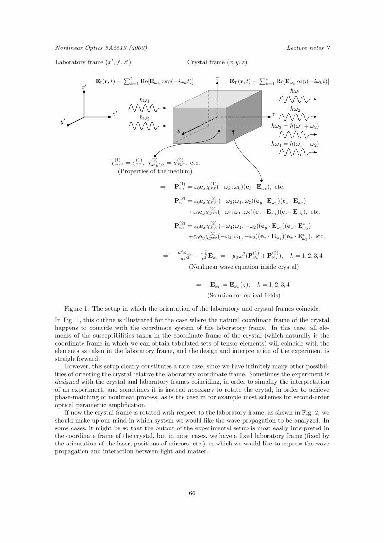
Nonlinear Optics 5A5513 (2003) Lecture notes 7
x′
y′z′
Laboratory frame (x′, y′, z′)
x
y
z
Crystal frame (x, y, z)
hω1
hω2
hω1
hω2
hω3 = h(ω1 + ω2)
hω4 = h(ω1 − ω2)
χ(1)x′x′ = χ
(1)xx , χ
(2)x′y′z′ = χ
(2)xyz, etc.
(Properties of the medium)
⇒ P(1)ωk = ε0exχ
(1)xx (−ωk;ωk)(ex · Eωk
), etc.
P(2)ω3 = ε0exχ
(2)xyz(−ω3;ω1, ω2)(ey · Eω1)(ez · Eω2)
+ε0eyχ(2)yxx(−ω3;ω1, ω2)(ex · Eω1)(ex · Eω2), etc.
P(2)ω4 = ε0exχ
(2)xyz(−ω4;ω1,−ω2)(ey · Eω1)(ez · E∗
ω2)
+ε0eyχ(2)yxx(−ω4;ω1,−ω2)(ex · Eω1)(ex · E∗
ω2), etc.
⇒ d2Eωk
dz′2 +ω2
k
c2 Eωk= −µ0ω
2(P(1)ωk + P
(2)ωk ), k = 1, 2, 3, 4
(Nonlinear wave equation inside crystal)
⇒ Eωk= Eωk
(z), k = 1, 2, 3, 4
(Solution for optical fields)
EI(r, t) =∑2k=1 Re[Eωk
exp(−iωkt)] ET(r, t) =∑4k=1 Re[Eωk
exp(−iωkt)]
Figure 1. The setup in which the orientation of the laboratory and crystal frames coincide.
In Fig. 1, this outline is illustrated for the case where the natural coordinate frame of the crystalhappens to coincide with the coordinate system of the laboratory frame. In this case, all ele-ments of the susceptibilities taken in the coordinate frame of the crystal (which naturally is thecoordinate frame in which we can obtain tabulated sets of tensor elements) will coincide with theelements as taken in the laboratory frame, and the design and interpretation of the experiment isstraightforward.
However, this setup clearly constitutes a rare case, since we have infinitely many other possibil-ities of orienting the crystal relative the laboratory coordinate frame. Sometimes the experiment isdesigned with the crystal and laboratory frames coinciding, in order to simplify the interpretationof an experiment, and sometimes it is instead necessary to rotate the crytal, in order to achievephase-matching of nonlinear process, as is the case in for example most schemes for second-orderoptical parametric amplification.
If now the crystal frame is rotated with respect to the laboratory frame, as shown in Fig. 2, weshould make up our mind in which system we would like the wave propagation to be analyzed. Insome cases, it might be so that the output of the experimental setup is most easily interpreted inthe coordinate frame of the crystal, but in most cases, we have a fixed laboratory frame (fixed bythe orientation of the laser, positions of mirrors, etc.) in which we would like to express the wavepropagation and interaction between light and matter.
66

Lecture notes 7 Nonlinear Optics 5A5513 (2003)
x′
y′z′
Laboratory frame (x′, y′, z′)
x
y
z
Crystal frame (x, y, z) [rotated relative (x′, y′, z′)]
hω1
hω2
(?)
hω1
(?)hω2
(?)
hω3 = h(ω
1 + ω2)
(?)
hω4 =h(ω
1 −ω
2 )
χ(1)x′x′ 6= χ
(1)xx , χ
(2)x′y′z′ 6= χ
(2)xyz, etc.
(Properties of the medium)
⇒ P(1)ωk =?
P(2)ω3 =?
P(2)ω4 =?
⇒ d2Eωk
dz′2 +ω2
k
c2 Eωk= −µ0ω
2(P(1)ωk + P
(2)ωk ) =? k = 1, 2, 3, 4
(Nonlinear wave equation inside crystal)
⇒ Eωk=?
(Solution for optical fields)
EI(r, t) =∑2k=1 Re[Eωk
exp(−iωkt)]
Figure 2. The setup in which the crystal frame is rotated relative the laboratory frame.
In Fig. 2, we would, in order to express the nonlinear process in the laboratory frame, like to
obtain the naturally appearing susceptibilities χ(2)xyz , χ
(2)xxx, etc., in the laboratory frame instead, as
χ(2)x′y′z′ , χ
(2)x′x′x′ , etc.
Just to summarize, why are then the transformation rules and spatial symmetries of the meduimso important?
• Hard to make physical conclusions about generated optical fields unless orientation of thelaboratory and crystal frames coincide.
• Spatial symmetries often significantly simplifies the wave propagation problem (by choosing asuitable polarization state and direction of propagation of the light, etc.).
• Useful for reducing the number of necessary elements of the susceptibility tensors (using Neu-mann’s principle).
Optical properties in rotated coordinate frames
Consider two coordinate systems described by Cartesian coordinates xα and x′α, respectively. Thecoordinate systems are rotated with respect to each other, and the relation between the coordinatesare described by the [3 × 3] transformation matrix Rab as
x′ = Rx ⇔ x′α = Rαβxβ , [B.& C. (5.40)]
where x = (x, y, z)T and x′ = (x′, y′, z′)T are column vectors. The inverse transformation betweenthe coordinate systems is similarly given as
x = R−1x′ ⇔ xβ = Rαβx′α. [B.& C. (5.41)]
67

Nonlinear Optics 5A5513 (2003) Lecture notes 7
x
y
z
x′
y′
z′
Figure 3. Illustration of proper rotation of the crystal frame (x, y, z) relative to the laboratoryreference frame (x′, y′, z′), by means of x′α = Rαβxβ with det (R) = 1.
xy
z
7−→
(a)
x′y′
z′
xy
z
7−→
(b)
x′y′
z′
Figure 4. The coordinate transformations (a) x = (x, y, z) 7→ x′ = (−x,−y, z), constituting aproper rotation around the z-axis, and (b) the space inversion x 7→ x′ = −x, an improper rotationcorresponding to, for example, a rotation around the z-axis followed by an inversion in the xy-plane.
We should notice that there are two types of rotations that are encountered as transformations:
• Proper rotations, for which det(R) = 1. (Righthanded systems keep being righthanded, andlefthanded systems keep being lefthanded.)
• Improper rotations, for which det(R) = −1. (Righthanded systems are transformed into left-handed systems, and vice versa.)
The electric field E(r, t) and electric polarization density P(r, t) are both polar quantities thattransform in the same way as regular Cartesian coordinates, and hence we have descriptions ofthese quantities in coordinate systems (x, y, z) and (x′, y′, z′) related to each other as
E′µ(r, t) = RµuEu(r, t) ⇔ Eu(r, t) = RµuE
′µ(r, t),
and
P ′µ(r, t) = RµuPu(r, t) ⇔ Pu(r, t) = RµuP
′µ(r, t),
respectively. Using these transformation rules, we will now derive the form of the susceptibilitiesin rotated coordinate frames.
First order polarization density in rotated coordinate frames
From the transformation rule for the electric polarization density above, using the standard form aswe previously have expressed the electric field dependence, we have for the first order polarization
68

Lecture notes 7 Nonlinear Optics 5A5513 (2003)
density in the primed coordinate system
P (1)µ
′(r, t) = RµuP(1)u (r, t)
= Rµuε0
∫ ∞
−∞
χ(1)ua (−ω;ω)Ea(ω) exp(−iωt) dω
= Rµuε0
∫ ∞
−∞
χ(1)ua (−ω;ω)RαaE
′α(ω) exp(−iωt) dω
= ε0
∫ ∞
−∞
χ(1)µα
′(−ω;ω)E′α(ω) exp(−iωt) dω
whereχ(1)µα
′(−ω;ω) = RµuRαaχ(1)ua (−ω;ω) [B.& C. (5.45)]
is the linear electric susceptibility taken in the primed coordinate system.
Second order polarization density in rotated coordinate frames
Similarly, we have the second order polarization density in the primed coordinate system as
P (2)µ
′(r, t) = RµuP(2)u (r, t)
= Rµuε0
∫ ∞
−∞
∫ ∞
−∞
χ(2)uab(−ωσ;ω1, ω2)Ea(ω1)Eb(ω2) exp[−i(ω1 + ω1)t] dω2 dω1
= Rµuε0
∫ ∞
−∞
∫ ∞
−∞
χ(2)uab(−ωσ;ω1, ω2)RαaE
′α(ω1)RβbE
′β(ω2) exp[−i(ω1 + ω1)t] dω2 dω1
= ε0
∫ ∞
−∞
∫ ∞
−∞
χ(2)µαβ
′(−ωσ;ω1, ω2)E′α(ω1)E
′β(ω2) exp[−i(ω1 + ω1)t] dω2 dω1
whereχ
(2)µαβ
′(−ωσ;ω1, ω2) = RµuRαaRβbχ(2)uab(−ωσ;ω1, ω2) [B.& C. (5.46)]
is the second order electric susceptibility taken in the primed coordinate system.
Higher order polarization densities in rotated coordinate frames
In a manner completely analogous to the second order susceptibility, the transformation rule be-tween the primed and unprimed coordinate systems can be obtained for the nth order elements ofthe electric susceptibility tensor as
χ(n)µα1···αn
′(−ωσ;ω1, . . . , ωn) = RµuRα1a1· · ·Rαnan
χ(n)ua1···an
(−ωσ;ω1, . . . , ωn). [B.& C. (5.47)]
Crystallographic point symmetry groups
Typically, a particular point symmetry group of the medium can be described by the generatingmatrices that describe the minimal set of transformation matrices (describing a set of symmetryoperations) that will be necessary for the reduction of the constitutive tensors. Two systems arewidely used for the description of point symmetry groups:2
• The International system, e. g. 43m, m3m, 422, etc.• The Schonflies system, e. g. Td, Oh, D4, etc.
The crystallographic point symmetry groups may contain any of the following symmetry oper-ations:
1. Rotations through integral multiples of 2π/n about some axis. The axis is called the n-foldrotation axis. It is in solid state physics shown [1–3] that a Bravais lattice can contain only 2-,3-, 4-, or 6-fold axes, and since the crystallographic point symmetry groups are contained in theBravais lattice point groups, they too can only have these axes.
2 C. f. Table 2 of the handed out Hartmann’s An Introduction to Crystal Physics.
69

Nonlinear Optics 5A5513 (2003) Lecture notes 7
2. Rotation-reflections. Even when a rotation through 2π/n is not a symmetry element,sometimes such a rotation followed by a reflection in a plane perpendicular to the axis may be asymmetry operation. The axis is then called an n-fold rotation-reflection axis. For example, thegroups S6 and S4 have 6- and 4-fold rotation-reflection axes.
3. Rotation-inversions. Similarly, sometimes a rotation through 2π/n followed by an inversionin a point lying on the rotation axis is a symmetry element, even though such a rotation by itselfis not. The axis is then called an n-fold rotation-inversion axis. However, the axis in S6 is only a3-fold rotation-inversion axis.
4. Reflections. A reflection takes every point into its mirror image in a plane, known as amirror plane.
5. Inversions. An inversion has a single fixed point. If that point is taken as the origin, thenevery other point r is taken into −r.
Schonflies notation for the non-cubic crystallographic point groups
The twenty-seven non-cubic crystallographic point symmetry groups may contain any of the fol-lowing symmetry operations, here given in Schonflies notation3:
Cn These groups contain only an n-fold rotation axis.
Cnv In addition to the n-fold rotation axis, these groups have a mirror plane that containsthe axis of rotation, plus as many additional mirror planes as the existence of then-fold axis requires.
Cnh These groups contain in addition to the n-fold rotation axis a single mirror planethat is perpendicular to the axis.
Sn These groups contain only an n-fold rotation-reflection axis.
Dn In addition to the n-fold rotation axis, these groups contain a 2-fold axis perpendic-ular to the n-fold rotation axis, plus as many additional 2-fold axes as are requiredby the existence of the n-fold axis.
Dnh These (the most symmetric groups) contain all the elements of Dn plus a mirrorplane perpendicular to the n-fold axis.
Dnd These contain the elements of Dn plus mirror planes containing the n-fold axis, whichbisect the angles between the 2-fold axes.
Neumann’s principle
Neumann’s principle simply states that any type of symmetry which is exhibited by the pointsymmetry group of the medium is also possessed by every physical property of the medium.
In other words, we can reformulate this for the optical properties as: the susceptibility tensorsof the medium must be left invariant under any transformation that also is a point symmetryoperation of the medium, or
χ(n)′
µα1···αn(−ωσ;ω1, . . . , ωn) = χ
(n)µα1···αn
(−ωσ;ω1, . . . , ωn),
where the tensor elements in the primed coordinate system are transformed according to
χ(n)′
µα1···αn(−ωσ;ω1, . . . , ωn) = RµuRα1a1
· · ·Rαnanχ
(n)ua1···an
(−ωσ;ω1, . . . , ωn),
where the [3 × 3] matrix R describes a point symmetry operation of the system.
3 In Schonflies notation, C stands for “cyclic”, D for “dihedral”, and S for “spiegel”. Thesubscripts h, v, and d stand for “horizontal”, “vertical”, and “diagonal”, respectively, and referto the placement of the placement of the mirror planes with respect to the n-fold axis, alwaysconsidered to be vertical. (The “diagonal” planes in Dnd are vertical and bisect the angles betweenthe 2-fold axes)
70
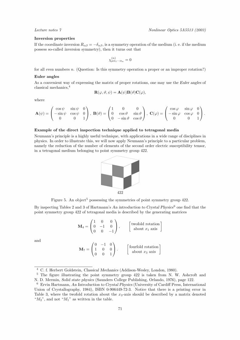
Lecture notes 7 Nonlinear Optics 5A5513 (2003)
Inversion properties
If the coordinate inversion Rαβ = −δαβ , is a symmetry operation of the medium (i. e. if the mediumpossess so-called inversion symmetry), then it turns out that
χ(n)µα1···αn
= 0
for all even numbers n. (Question: Is this symmetry operation a proper or an improper rotation?)
Euler angles
As a convenient way of expressing the matrix of proper rotations, one may use the Euler angles ofclassical mechanics,4
R(ϕ, ϑ, ψ) = A(ψ)B(ϑ)C(ϕ),
where
A(ψ) =
cosψ sinψ 0− sinψ cosψ 0
0 0 1
, B(ϑ) =
1 0 00 cosϑ sinϑ0 − sinϑ cosϑ
, C(ϕ) =
cosϕ sinϕ 0− sinϕ cosϕ 0
0 0 1
.
Example of the direct inspection technique applied to tetragonal media
Neumann’s principle is a highly useful technique, with applications in a wide range of disciplines inphysics. In order to illustrate this, we will now apply Neumann’s principle to a particular problem,namely the reduction of the number of elements of the second order electric susceptibility tensor,in a tetragonal medium belonging to point symmetry group 422.
422
Figure 5. An object5 possessing the symmetries of point symmetry group 422.
By inspecting Tables 2 and 3 of Hartmann’s An introduction to Crystal Physics6 one find that thepoint symmetry group 422 of tetragonal media is described by the generating matrices
M4 =
1 0 00 −1 00 0 −1
,
[twofold rotationabout x1 axis
]
and
M7 =
0 −1 01 0 00 0 1
.
[fourfold rotationabout x3 axis
]
4 C. f. Herbert Goldstein, Classical Mechanics (Addison-Wesley, London, 1980).5 The figure illustrating the point symmetry group 422 is taken from N. W. Ashcroft and
N. D. Mermin, Solid state physics (Saunders College Publishing, Orlando, 1976), page 122.6 Ervin Hartmann, An Introduction to Crystal Physics (University of Cardiff Press, International
Union of Crystallography, 1984), ISBN 0-906449-72-3. Notice that there is a printing error inTable 3, where the twofold rotation about the x3-axis should be described by a matrix denoted“M2”, and not “M1” as written in the table.
71
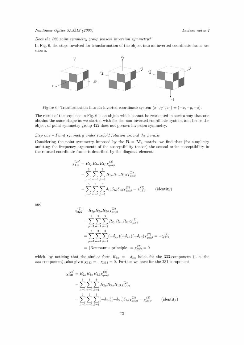
Nonlinear Optics 5A5513 (2003) Lecture notes 7
Does the 422 point symmetry group possess inversion symmetry?
In Fig. 6, the steps involved for transformation of the object into an inverted coordinate frame areshown.
x1
x2
x3
x′1x′2
x′3
x′′1x′′2
x′′3
Figure 6. Transformation into an inverted coordinate system (x′′, y′′, z′′) = (−x,−y,−z).
The result of the sequence in Fig. 6 is an object which cannot be reoriented in such a way that oneobtains the same shape as we started with for the non-inverted coordinate system, and hence theobject of point symmetry group 422 does not possess inversion symmetry.
Step one – Point symmetry under twofold rotation around the x1-axis
Considering the point symmetry imposed by the R = M4 matrix, we find that (for simplicityomitting the frequency arguments of the susceptibility tensor) the second order susceptibility inthe rotated coordinate frame is described by the diagonal elements
χ(2)′
111 = R1µR1αR1βχ(2)µαβ
=
3∑
µ=1
3∑
α=1
3∑
β=1
R1µR1αR1βχ(2)µαβ
=3∑
µ=1
3∑
α=1
3∑
β=1
δ1µδ1αδ1βχ(2)µαβ = χ
(2)111, (identity)
and
χ(2)′
222 = R2µR2αR2βχ(2)µαβ
=
3∑
µ=1
3∑
α=1
3∑
β=1
R2µR2αR2βχ(2)µαβ
=3∑
µ=1
3∑
α=1
3∑
β=1
(−δ2µ)(−δ2α)(−δ2β)χ(2)µαβ = −χ(2)
222
= Neumann′s principle = χ(2)222 = 0
which, by noticing that the similar form R3α = −δ3α holds for the 333-component (i. e. thezzz-component), also gives χ333 = −χ333 = 0. Further we have for the 231-component
χ(2)′
231 = R2µR3αR1βχ(2)µαβ
=
3∑
µ=1
3∑
α=1
3∑
β=1
R2µR3αR1βχ(2)µαβ
=3∑
µ=1
3∑
α=1
3∑
β=1
(−δ2µ)(−δ3α)δ1βχ(2)µαβ = χ
(2)231, (identity)
72

Lecture notes 7 Nonlinear Optics 5A5513 (2003)
etc., and by continuing in this manner for all 27 elements of χ(2)′
µαβ , one finds that the symmetryoperation R = M4 leaves us with the tensor elements listed in Table 1.
Zero elements Identities (no further info)
χ(2)112, χ
(2)113, χ
(2)121, χ
(2)131,
χ(2)211, χ
(2)222, χ
(2)223, χ
(2)232, (all other 13 elements)
χ(2)233, χ
(2)311, χ
(2)322, χ
(2)323,
χ(2)332, χ
(2)333
Table 1. Reduced set of tensor elements after the symmetry operation R = M4.
Step two – Point symmetry under fourfold rotation around the x3-axis
Proceeding with the next point symmetry operation, described by R = M7, one finds for theremaining 13 elements that, for example, for the 123-element
χ(2)′
123 = R1µR2αR3βχ(2)µαβ
=
3∑
µ=1
3∑
α=1
3∑
β=1
R1µR2αR3βχ(2)µαβ
=3∑
µ=1
3∑
α=1
3∑
β=1
(−δ2µ)δ1αδ3βχ(2)µαβ = −χ(2)
213
= Neumann′s principle = χ(2)123,
and for the 132-element
χ(2)′
132 = R1µR3αR2βχ(2)µαβ
=
3∑
µ=1
3∑
α=1
3∑
β=1
R1µR3αR2βχ(2)µαβ
=3∑
µ=1
3∑
α=1
3∑
β=1
(−δ2µ)δ3αδ1βχ(2)µαβ = −χ(2)
231
= Neumann′s principle = χ(2)132,
while the 111-element (which previously, by using the R = M4 point symmetry, just gave anidentity with no further information) now gives
χ(2)′
111 = R1µR1αR1βχ(2)µαβ
=
3∑
µ=1
3∑
α=1
3∑
β=1
R1µR1αR1βχ(2)µαβ
=
3∑
µ=1
3∑
α=1
3∑
β=1
(−δ2µ)(−δ2α)(−δ2β)χ(2)µαβ = −χ(2)
222
= from previous result for χ(2)222 = 0
= Neumann′s principle = χ(2)111.
By (again) proceeding for all 27 elements of χ(2)′
µαβ , one finds the set of tensor elements as listed in
73

Nonlinear Optics 5A5513 (2003) Lecture notes 7
Table 2. (See also the tabulated set in Butcher and Cotter’s book, Table A3.2, page 299.)
Zero elements Nonzero elements
χ(2)111, χ
(2)112, χ
(2)113, χ
(2)121, χ
(2)122, χ
(2)123 = −χ(2)
213,
χ(2)131, χ
(2)133, χ
(2)211, χ
(2)212, χ
(2)221, χ
(2)132 = −χ(2)
231,
χ(2)222, χ
(2)223, χ
(2)232, χ
(2)233, χ
(2)311, χ
(2)321 = −χ(2)
312,
χ(2)313, χ
(2)322, χ
(2)323, χ
(2)331, χ
(2)332, χ
(2)333 (6 nonzero, 3 independent)
Table 2. Reduced set of tensor elements after symmetry operations R = M4 and R = M7.
74

Lecture Notes on Nonlinear Optics Nonlinear Optics 5A5513 (2003)
Lecture VIII
75

Nonlinear Optics 5A5513 (2003) Lecture Notes on Nonlinear Optics
Lecture Notes on Nonlinear OpticsNonlinear Optics (5A5513, 5p for advanced undergraduate and doctoral students)Course given at the Royal Institute of Technology,Department of Laser Physics and Quantum OpticsSE–106 91, Stockholm, SwedenJanuary 8 – March 24, 2003
The texts and figures in this lecture series was typeset by the author in 10/12/16 pt ComputerModern typeface using plain TEX and METAPOST.
This document is electronically available at the homepage of the Library of the Royal Institute ofTechnology, at http://www.lib.kth.se.
Copyright c© Fredrik Jonsson 2003
All rights reserved. No part of this publication may be reproduced, stored in a retrieval system,or transmitted, in any form, or by any means, electronic, mechanical, photo-copying, recording, orotherwise, without the prior consent of the author.
ISBN 91-7283-517-6TRITA-FYS 2003:26ISSN 0280-316XISRN KTH/FYS/- - 03:26 - - SEPrinted on July 7, 2003
TEX is a trademark of the American Mathematical Society
76

Nonlinear Optics 5A5513 (2003)Lecture notes
Lecture 8
In this lecture, the electric polarisation density of the medium is finally inserted into Maxwell’sequations, and the wave propagation properties of electromagnetic waves in nonlinear optical mediais for the first time in this course analysed. As an example of wave propagation in nonlinear opticalmedia, the optical Kerr effect is analysed for infinite plane continuous waves.
The outline for this lecture is:• Maxwells equations (general electromagnetic wave propagation)• Time dependent processes (envelopes slowly varying in space and time)• Time independent processes (envelopes slowly varying in space but constant in time)
• Examples (optical Kerr-effect ⇔ χ(3)µαβγ(−ω;ω, ω,−ω))
Wave propagation in nonlinear media
Maxwell’s equations
The propagation of electromagnetic waves are, from a first principles approach, governed by theMaxwell’s equations (here listed in their real-valued form in SI units),
∇× E(r, t) = −∂B(r, t)
∂t, (Faraday′s law)
∇× H(r, t) = J(r, t) +∂D(r, t)
∂t, (Ampere′s law)
∇ · D(r, t) = ρ(r, t),
∇ · B(r, t) = 0,
where ρ(r, t) is the density of free charges, and J(r, t) the corresponding current density of freecharges.
Constitutive relations
The constitutive relations are in SI units formulated as
D(r, t) = ε0E(r, t) + P(r, t),
B(r, t) = µ0[H(r, t) + M(r, t)],
where P(r, t) = P[E(r, t),B(r, t)] is the macroscopic polarization density (electric dipole momentper unit volume), and M(r, t) = M[E(r, t),B(r, t)] the magnetization (magnetic dipole momentper unit volume) of the medium.
Here E(r, t) and B(r, t) are considered as the fundamental macroscopic electric and magneticfield quantities; D(r, t) and H(r, t) are the corresponding derived fields associated with the stateof matter, connected to E(r, t) and B(r, t) through the electric polarization density P(r, t) andmagnetization (magnetic polarization density) M(r, t) through the basic constitutive relations. Infact, the constitutive equations above form the very definitions1 of the electric polarization densityand magnetization.
1 J. D. Jackson, Classical Electrodynamics, 2nd ed. (Wiley, New York, 1975); J. A. Stratton,Electromagnetic Theory (McGraw-Hill, New York, 1941).
77
Nonlinear Optics 5A5513 (2003) Lecture notes 8
Two frequent assumptions in nonlinear optics
• No free charges present,
ρ(r, t) = 0, J(r, t) = 0.
(Any relaxation processes etc. are included in imaginary parts of the terms of the electricsusceptibility.)
• No magnetization of the medium,
M(r, t) = 0.
The wave equation
By taking the cross product with the nabla operator and Faraday’s law, one obtains
∇×∇× E(r, t) = − ∂
∂t∇× B(r, t)
= −µ0∂
∂t∇× H(r, t)
= −µ0∂
∂t
∂D(r, t)
∂t
= −µ0
(ε0∂2E(r, t)
∂t2+∂2P(r, t)
∂t2
).
Since now µ0ε0 = 1/c2 in SI units, with c being the speed of light in vacuum, one hence obtainsthe basic wave equation, taken in time domain, as
∇×∇× E(r, t) +1
c2∂2E(r, t)
∂t2= −µ0
∂2P(r, t)
∂t2, (1)
where, as in the previous lectures of this course, the polarization density can be written in termsof the perturbation series as
P(r, t) =∞∑
k=1
P(k)(r, t) = ε0
∫ ∞
−∞
χ(1)µα(−ω;ω)Eα(r, ω) exp(−iωt) dω
︸ ︷︷ ︸=P(1)(r,t)
+∞∑
k=2
P(k)(r, t)
︸ ︷︷ ︸=P(NL)(r,t)
In the left hand side of Eq. (1), we find the part of the homogeneous wave equation for propagationof electromagnetic waves in vacuum, while the right hand side described the modifications to thevacuum propagation due to the interaction between light and matter. In this respect, it is nowclear that the electric polarisation effectively acts as a source term in the mathematical descriptionof electromagnetic wave propagation, making the otherwise homogeneous vacuum problem aninhomogeneous problem (though with known source terms).
It should be noticed that whenever the polarization density is calculated from the Bloch equa-tions (formulated later on, in lecture 10 of this course), instead of by means of a perturbationseries as above, the Maxwell equations and the wave equation (1) above are denoted Maxwell-Bloch equations. In some sense, we can therefore see the choice of method for the calculation ofthe polarization density as a switch point not only for using the susceptibility formalism or not forthe description of interaction between light and matter, but also for the form of the wave propa-gation problem in nonlinear media, which mathematically significantly differ between the “pure”Maxwell’s equations with susceptibilities and the Maxwell-Bloch equations.
78

Lecture notes 8 Nonlinear Optics 5A5513 (2003)
The wave equation in frequency domain (optional)
Frequently in this course, we have rather been studying the electric fields and polarisation densitiesin frequency domain, since many phenomena in optics are properly and conveniently described asstatic (in which case the frequency dependence is simply reduced to the interaction between discretefrequencies in the spectrum). By using the Fourier integral identity2
Eα(t) =
∫ ∞
−∞
Eα(ω) exp(−iωt) dω = F−1[Eα](t),
with inverse relation
Eα(ω) =1
2π
∫ ∞
−∞
Eα(τ) exp(iωτ) dτ = F[Eα](ω),
we obtain the wave equation (1) as
∇×∇× E(r, ω) − ω2
c2E(r, ω) = µ0ω
2P(r, ω).
Quasimonochromatic light - Time dependent problems
By inserting the perturbation series for the electric polarisation density into the general waveequation (1), which apply to arbitrary electric field distributions and field intensities of the light,one obtains the equation
∇×∇× E(r, t) +1
c2∂2
∂t2
∫ ∞
−∞
eµεµα(ω)Eα(r, ω) exp(−iωt) dω︸ ︷︷ ︸
(denote this integral as I for later use)
= −µ0∂2P(NL)(r, t)
∂t2, (2)
whereεµα(ω) = δµα + χ(1)
µα(−ω;ω)
is a parameter commonly denoted as the relative electrical permittivity.3 This wave equation isidentical to Eq. (7.14) in Butcher and Cotter’s book. (Notice though the printing error in Butcherand Cotter’s Eq. (7.14), where the first µ0 should be replaced by 1/c2.)
The second term of the left hand side of Eq. (2) gives all first order optical contributions tothe wave propagation, as well as all linear optical dispersion effects. This terms deserves someextra attention, and we will now proceed with deriving the effect of the frequency dependence ofthe relative permittivity upon the wave equation. First of all, we notice that since Eα(r,−ω) =E∗α(r, ω), which simply is a consequence of the choice of complex Fourier transform of a real valued
field, the reality condition of Eq. (2) requires that
εµα(−ω) = ε∗µα(ω).
2 From the inverse Fourier integral identity, it follows that the Fourier transform of a derivativeof a function f(t) is
F[f ′(t)](ω) = −iω F[f(t)](ω) ⇒ F[f ′′(t)](ω) = −ω2F[f(t)](ω).
3 Notice that for isotropic media, χ(1)µα(−ω;ω) = χ
(1)xx (−ω;ω)δµα, which leads to the simplified
formeµεµα(ω)Eα(r, ω) = ε(ω)E(r, ω).
We will here, however, continue with the general form, in order not to loose generality in discussionthat is to follow.
79

Nonlinear Optics 5A5513 (2003) Lecture notes 8
It should be emphasized that this property of the relative electrical permittivity merely is a conve-nient mathematical construction, since we in regular physical terms only consider positive angularfrequencies as argument for the refractive index, etc.
For quasimonochromatic light, the electric field and polarisation density are taken as
E(r, t) =∑
ωσ≥0
Re[Eωσ(r, t) exp(−iωσt)],
P(r, t) =∑
ωσ≥0
Re[Pωσ(r, t) exp(−iωσt)],
where Eωσ(r, t) and Pωσ
(r, t) are slowly varying envelopes of the fields. In the frequency domain,the quasimonochromatic fields are expressed as
E(r, ω) =1
2
∑
ωσ≥0
[Eωσ(r, ω − ωσ) + E∗
ωσ(r,−ω − ωσ)],
P(r, ω) =1
2
∑
ωσ≥0
[Pωσ(r, ω − ωσ) + P∗
ωσ(r,−ω − ωσ)],
where the envelopes have some limited extent around the carrier frequencies at ±ωσ. Notice thatthe fields taken in the frequency domain are expressed entirely in terms of their respective temporalenvelope, that is to say, without the exponential functions that appear in their counterparts in timedomain.
For simplicity considering a medium that in the linear optical domain is isotropic, with therelative electrical permittivity
εµα(ω) = ε(ω)δµα = n20(ω)δµα,
where n0(ω) is the first order contribution to the refractive index of the medium, this leads to themiddle term of the wave equation (1) in the form
I ≡ 1
c2∂2
∂t2
∫ ∞
−∞
eµεµα(ω)Eα(r, ω) exp(−iωt) dω
= −∫ ∞
−∞
ω2n2(ω)
c21
2
∑
ωσ≥0
[Eωσ(r, ω − ωσ) + E∗
ωσ(r,−ω − ωσ)]
︸ ︷︷ ︸quasimonochromatic form of E(r,ω)
exp(−iωt) dω
= denote ω2ε(ω)/c2 ≡ ω2n20(ω)/c2 ≡ k2(ω)
= −1
2
∑
ωσ≥0
∫ ∞
−∞
k2(ω)[Eωσ(r, ω − ωσ) + E∗
ωσ(r,−ω − ωσ)] exp(−iωt) dω.
= −1
2
∑
ωσ≥0
∫ ∞
−∞
k2(ω)Eωσ(r, ω − ωσ) exp(−iωt) dω + c. c.
If now the field envelopes decay to zero rapidly enough in the vicinity of the carrier frequencies(as we would expect for quasimonochromatic light, with a strong spectral confinement around thecarrier frequency of the light), then we may expect that a good approximation is to make a Taylorexpansion of k2(ω), in the neighbourhood of respective carrier frequency of the light, as
k2(ω) ≈(k(ωσ) +
dk
dω
∣∣∣ωσ
(ω − ωσ) +1
2!
d2k
dω2
∣∣∣ωσ
(ω − ωσ)2)2
≈ k2σ + 2kσ
dk
dω
∣∣∣ωσ
(ω − ωσ) + kσd2k
dω2
∣∣∣ωσ
(ω − ωσ)2,
80

Lecture notes 8 Nonlinear Optics 5A5513 (2003)
where the notation kσ = k(ωσ) was introduced, and hence4
I ≈ −1
2
∑
ωσ≥0
∫ ∞
−∞
(k2σ + 2kσ
dk
dω
∣∣∣ωσ
(ω − ωσ) + kσd2k
dω2
∣∣∣ωσ
(ω − ωσ)2)
× Eωσ(r, ω − ωσ) exp(−iωt) dω + c. c.
= change variable of integration ω′ = ω − ωσ
= −1
2
∑
ωσ≥0
∫ ∞
−∞
(k2σ + 2kσ
dk
dω
∣∣∣ωσ
ω′ + kσd2k
dω2
∣∣∣ωσ
ω′2)
× Eωσ(r, ω′) exp(−iω′t) dω′ exp(−iωσt) + c. c.
=
use
∫ ∞
−∞
ωnf(ω) exp(−iωt) dω = F−1[ωnf(ω)](t) = in
dnf(t)
dtn
= −1
2
∑
ωσ≥0
exp(−iωσt)(k2σ + i2kσ
dk
dω
∣∣∣ωσ
∂
∂t− kσ
d2k
dω2
∣∣∣ωσ
∂2
∂t2
)Eωσ
(r, t) + c. c.
As this result is inserted back into the wave equation (2), one obtains
1
2
∑
ωσ≥0
exp(−iωσt)[∇×∇× Eωσ
(r, t)
−(k2σ + 2ikσ
dk
dω
∣∣∣ωσ
∂
∂t− kσ
d2k
dω2
∣∣∣ωσ
∂2
∂t2
)Eωσ
(r, t)]
+ c. c.
= −µ0∂2P(NL)(r, t)
∂t2
= −µ0∂2
∂t21
2
∑
ωσ≥0
P(NL)ωσ
(r, t) exp(−iωσt) + c. c.
≈ µ01
2
∑
ωσ≥0
ω2σP
(NL)ωσ
(r, t) exp(−iωσt) + c. c.
As we separate out the respective frequency components at ω = ωσ of this equation, one obtainsthe time dependent wave equation for the temporal envelope components of the electric field as
∇×∇× Eωσ(r, t) −
(k2σ + i2kσ
1
vg
∂
∂t− kσ
d2k
dω2
∣∣∣ωσ
∂2
∂t2
)Eωσ
(r, t) = µ0ω2σP
(NL)ωσ
(r, t), (3)
where
vg =( dkdω
∣∣∣ωσ
)−1
.
4 Notice that unless we apply the second approximation in the Taylor expansion of k2(ω), termscontaining the squares of the derivatives will appear, which will lead to wave equations that differfrom the ones given by Butcher and Cotter. In particular, this situation will arise even if one usesthe suggested expansion given by Eq. (7.23) in Butcher and Cotter’s book, which hence should betaken with some care if one wish to build a strict foundation for the time-dependent wave equation.
81

Nonlinear Optics 5A5513 (2003) Lecture notes 8
Three practical approximations
[1] The infinite plane wave approximation,
Eωσ(r, t) = Eωσ
(z, t)⊥ez ⇒ ∇×∇× → − ∂2
∂z2.
[2] Unidirectional propagation,
Eωσ(z, t) = Aωσ
(z, t) exp(±ikσz)⇓
∇×∇× Eωσ(z, t) = −[
∂2Aωσ
∂z2± 2ikσ
∂Aωσ
∂z− k2
σAωσ] exp(±ikσz),
for waves propagating in the positive/negative z-direction. In this case, the real-valued electricfield hence takes the form
E(r, t) =∑
ωσ≥0
Re[Eωσ(r, t) exp(−iωσt)]
=∑
ωσ≥0
Re[Aωσ(z, t) exp(±ikσz − iωσt)]
=∑
ωσ≥0
|Aωσ(z, t)|Reexp[ikσz ∓ iωσt+ iφ(z)]
=∑
ωσ≥0
|Aωσ(z, t)| cos(kσz ∓ ωσt+ φ(z)),
where φ(z, t) describes the spatially and temporally varying phase of the complex-valued slowlyvarying envelope function Aωσ
(z, t) of the electric field.
[3] The slowly varying envelope approximation,
∣∣∣∂2Aωσ
∂z2
∣∣∣ ∣∣∣kσ
∂Aωσ
∂z
∣∣∣.
These approximations, whenever applicable, further reduce the time dependent wave equation to
(± i
∂
∂z+ i
1
vg
∂
∂t− 1
2
d2k
dω2
∣∣∣ωσ
∂2
∂t2
)Aωσ
(z, t) = −µ0ω2σ
2kσP(NL)ωσ
(r, t) exp(∓ikσz). (4)
This form of the wave equation is identical to Butcher and Cotter’s Eq. (7.24), with the exceptionthat here waves propagating in positive (upper signs) as well as negative (lower signs) z-directionare considered.
82
Lecture notes 8 Nonlinear Optics 5A5513 (2003)
Monochromatic light
Monochromatic optical field
E(r, t) =∑
σ
Re[Eωσ(r) exp(−iωσt)], ωσ ≥ 0
E(r, ω) =1
2
∑
σ
[Eωσ(r)δ(ω − ωσ) + E∗
ωσ(r)δ(ω + ωσ)]
Polarization density induced by monochromatic optical field
P(n)(r, t) =∑
ωσ≥0
Re[P(n)ωσ
exp(−iωσt)], ωσ = ω1 + ω2 + . . .+ ωn
(For construction of P(n)ωσ , see notes on the Butcher and Cotter convention handed out during the
third lecture.)
Monochromatic light - Time independent problems
For strictly monochromatic light, as for example the output light of continuous wave lasers, thetemporal field envelopes are constants in time, and the wave equation (3) is reduced to
∇×∇× Eωσ(r) − k2
σEωσ(r) = µ0ω
2σP
(NL)ωσ
(r). (5)
By applying the above listed approximations, one immediately finds the monochromatic, timeindependent form of Eq. (3) in the infinite plane wave limit and slowly varying approximation as
∂
∂zAωσ
= ±iµ0ω2σ
2kσP(NL)ωσ
exp(∓ikσz), (6)
where the upper/lower sign correspond to a wave propagating in the positive/negative z-direction.This equation corresponds to Butcher and Cotter’s Eq. (7.17).
83

Nonlinear Optics 5A5513 (2003) Lecture notes 8
Example I: Optical Kerr-effect - Time independent case
In this example, we consider continuous wave propagation5 in optical Kerr-media, using lightpolarized in the x-direction and propagating along the positive direction of the z-axis,
E(r, t) = Re[Eω(z) exp(−iωt)], Eω(z) = Aω(z) exp(ikz) = exAxω(z) exp(ikz),
where, as previously, k = ωn0/c. From material handed out during the third lecture (notes on theButcher and Cotter convention), the nonlinear polarization density for x-polarized light is given
as P(NL)ω = P
(3)ω , with
P(3)ω = ε0(3/4)exχ
(3)xxxx(−ω;ω, ω,−ω)|Exω|2Exω
= ε0(3/4)χ(3)xxxx|Eω|2Eω
= ε0(3/4)χ(3)xxxx|Aω|2Aω exp(ikz),
and the time independent wave equation for the field envelope Aω, using Eq. (6), becomes
∂
∂zAω = i
µ0ω2
2kε0(3/4)χ
(3)xxxx|Aω|2Aω exp(ikz)︸ ︷︷ ︸
=P(NL)ω (z)
exp(−ikz)
= i3ω2
8c2kχ(3)xxxx|Aω|2Aω
= since k = ωn0(ω)/c
= i3ω
8cn0χ(3)xxxx|Aω|2Aω
= in analogy with Butcher and Cotter Eq. (6.63), n2 = (3/8n0)χ(3)xxxx
= iωn2
c|Aω|2Aω,
or, equivalently, in its scalar form
∂
∂zAxω = i
ωn2
c|Axω|2Axω.
If the medium of interest now is analyzed at an angular frequency far from any resonance, we maylook for solutions to this equation with |Aω| being constant (for a lossless medium). For such acase it is straightforward to integrate the final wave equation to yield the general solution
Aω(z) = Aω(z0) exp[iωn2|Aω(z0)|2z/c],
or, again equivalently, in the scalar form
Axω(z) = Axω(z0) exp[iωn2|Axω(z0)|2z/c],
which hence gives the solution for the real-valued electric field E(r, t) as
E(r, t) = Re[Eω(z) exp(−iωt)]= ReAω(z) exp[i(kz − ωt)]= ReAω(z0) exp[i(kz + ωn2|Aω(z0)|2z/c− ωt)].
From this solution, one immediately finds that the wave propagates with an effective propagationconstant
k + ωn2|Aω(z0)|2/c = (ω/c)(n0 + n2|Aω(z0)|2),that is to say, experiencing the intensity dependent refractive index
neff = n0 + n2|Aω(z0)|2.
5 That is to say, a time independent problem with the temporal envelope of the electrical fieldbeing constant in time.
84

Lecture notes 8 Nonlinear Optics 5A5513 (2003)
Example II: Optical Kerr-effect - Time dependent case
We now consider a time dependent envelope Eω(z, t), of an optical wave propagating in the samemedium and geometry as in the previous example, for which now
E(r, t) = Re[Eω(z, t) exp(−iωt)], Eω(z, t) = Aω(z, t) exp(ikz) = exAxω(z, t) exp(ikz).
The proper wave equation to apply for this case is the time dependent wave equation (4), and sincethe nonlinear polarization density of the medium still is given by the optical Kerr-effect, we obtain
(i∂
∂z+ i
1
vg
∂
∂t− 1
2
d2k
dω2
∣∣∣ωσ
∂2
∂t2
)Aω(z, t)
= −µ0ω2
2kε0(3/4)χ
(3)xxxx|Aω(z, t)|2Aω(z, t) exp(ikz)︸ ︷︷ ︸
=P(NL)ω (z,t)
exp(−ikz)
= − 3ω2
8c2kχ(3)xxxx|Aω(z, t)|2Aω(z, t)
= as in previous example= −ωn2
c|Aω(z, t)|2Aω(z, t).
The resulting wave equation
(i∂
∂z+ i
1
vg
∂
∂t− 1
2
d2k
dω2
∣∣∣ωσ
∂2
∂t2
)Aω = −ωn2
c|Aω|2Aω
is the starting point for analysis of solitons and solitary waves in optical Kerr-media. The obtainedequation is the non-normalized form of the in nonlinear physics (not only nonlinear optics!) oftenencountered nonlinear Schrodinger equation (or NLSE, as its common acronym yields).
For a discussion on the transformation that cast the nonlinear Schrodinger equation into thenormalized nonlinear Schrodinger equation, see Butcher and Cotter’s book, page 240.
85

Nonlinear Optics 5A5513 (2003) Lecture notes 8
86

Lecture Notes on Nonlinear Optics Nonlinear Optics 5A5513 (2003)
Lecture IX
87
Nonlinear Optics 5A5513 (2003) Lecture Notes on Nonlinear Optics
Lecture Notes on Nonlinear OpticsNonlinear Optics (5A5513, 5p for advanced undergraduate and doctoral students)Course given at the Royal Institute of Technology,Department of Laser Physics and Quantum OpticsSE–106 91, Stockholm, SwedenJanuary 8 – March 24, 2003
The texts and figures in this lecture series was typeset by the author in 10/12/16 pt ComputerModern typeface using plain TEX and METAPOST.
This document is electronically available at the homepage of the Library of the Royal Institute ofTechnology, at http://www.lib.kth.se.
Copyright c© Fredrik Jonsson 2003
All rights reserved. No part of this publication may be reproduced, stored in a retrieval system,or transmitted, in any form, or by any means, electronic, mechanical, photo-copying, recording, orotherwise, without the prior consent of the author.
ISBN 91-7283-517-6TRITA-FYS 2003:26ISSN 0280-316XISRN KTH/FYS/- - 03:26 - - SEPrinted on July 7, 2003
TEX is a trademark of the American Mathematical Society
88

Nonlinear Optics 5A5513 (2003)Lecture notes
Lecture 9
In this lecture, we will focus on examples of electromagnetic wave propagation in nonlinear opticalmedia, by applying the forms of Maxwell’s equations as obtained in the eighth lecture to a set ofparticular nonlinear interactions as described by the previously formulated nonlinear susceptibilityformalism.
The outline for this lecture is:• General process for solving problems in nonlinear optics• Second harmonic generation (SHG)• Optical Kerr-effect
General process for solving problems in nonlinear optics
The typical steps in the process of solving a theoretical problem in nonlinear optics typicallyinvolve:
define the optical interaction of interest(identifying the susceptibility)
⇓
define in which medium the interaction take place(identify crystallographic point symmetry group)
⇓
consider eventual additional symmetries and constraints(e. g. intrinsic, overall, or Kleinman symmetries)
⇓
construct the polarization density(the Butcher and Cotter convention)
⇓
formulate the proper wave equation(e. g. taking dispersion or diffraction into account)
⇓
formulate the proper boundaryconditions for the wave equation
⇓
solve the wave equation underthe boundary conditions
89
Nonlinear Optics 5A5513 (2003) Lecture notes 9
Formulation of the exercises in this lecture
In order to illustrate the scheme as previously outlined, the following exercises serve as to givethe connection between the susceptibilities, as extensively analysed from a quantum-mechanicalbasis in earlier lectures of this course, and the wave equation, derived from Maxwell’s equations ofmotion for electromagnetic fields.
Exercise 1. (Second harmonic generation in negative uniaxial media) Consider a continuous pumpwave at angular frequency ω, initially polarized in the y-direction and propagating in the positivex-direction of a negative uniaxial crystal of crystallographic point symmetry group 3m. (Examplesof crystals belonging to this class: beta-BaB2O4/BBO, LiNbO3.)
1a. Formulate the polarization density of the medium for the pump and second harmonic wave.1b. Formulate the system of equations of motion for the electromagnetic fields.1c. Assuming no second harmonic signal present at the input, solve the equations of motion for
the second harmonic field, using the non-depleted pump approximation, and derive an expressionfor the conversion efficiency of the second harmonic generation.
Exercise 2. (Optical Kerr-effect – continuous wave case) In this setup, a monochromatic opticalwave is propagating in the positive z-direction of an isotropic optical Kerr-medium.
2a. Formulate the polarization density of the medium for a wave polarized in the xy-plane.2b. Formulate the polarization density of the medium for a wave polarized in the x-direction.2c. Formulate the wave equation for continuous wave propagation in optical Kerr-media. The
continuous wave is x-polarized and propagates in the positive z-direction.2d. For lossless media, solve the wave equation and give an expression for the nonlinear,
intensity-dependent refractive index n = n0 + n2|Eω|2.
90

Lecture notes 9 Nonlinear Optics 5A5513 (2003)
Second harmonic generation
The optical interaction
In the case of second harmonic generation (SHG), two photons at angular frequency ω combine toa photon at twice the angular frequency,
~ω + ~ω → ~(2ω).
This interaction is for the second harmonic wave (at angular frequency ω)described by the secondorder susceptibility
χ(2)µαβ(−ωσ;ω, ω),
where ωσ = 2ω is the generated second harmonic frequency of the light.
Symmetries of the medium
In this example we consider second harmonic generation in trigonal media of crystallographic pointsymmetry group 3m. (Example: LiNbO3)
y
x
z Crystal frame (x, y, z)
point symmetry group 3m
(e. g. LiNbO3)
EI(r, t) = Re[Eω exp(−iωt)]= eyRe[Eyω exp(−iωt)]
ET(r, t) = Re[Eω exp(−iωt)] + Re[E2ω exp(−i2ωt)]
Figure 1. The setup for optical second harmonic generation in LiNbO3.
For this point symmetry group, the nonzero tensor elements of the first order susceptibility are(for example according to Table A3.1 in The Elements of Nonlinear Optics)
χ(1)xx = χ(1)
yy , χ(1)zz ,
which gives the ordinary refractive indices
nx(ω) = ny(ω) = [1 + χ(1)xx (−ω;ω)]1/2 ≡ nO(ω)
for waves components polarized in the x- or y-directions, and the extraordinary refractive index
nz(ω) = [1 + χ(1)zz (−ω;ω)]1/2 ≡ nE(ω)
for the wave component polarized in the z-direction. Since we here are considering a negativelyuniaxial crystal (see Butcher and Cotter, p. 214), these refractive indices satisfy the inequality
nE(ω) ≤ nO(ω).
The nonzero tensor elements of the second order susceptibility are (for example according toTable A3.2 in The Elements of Nonlinear Optics)
χ(2)yxx = χ(2)
xyx = χ(2)xxy = −χ(2)
yyy , χ(2)zzz ,
χ(2)zxx = χ(2)
zyy, χ(2)yyz = χ(2)
xxz , χ(2)yzy = χ(2)
xzx,(1)
91

Nonlinear Optics 5A5513 (2003) Lecture notes 9
Additional symmetries
Intrinsic permutation symmetry for the case of second harmonic generation gives
χ(2)xxz(−2ω;ω, ω) = χ(2)
xzx(−2ω;ω, ω) = χ(2)yzy(−2ω;ω, ω) = χ(2)
yyz(−2ω;ω, ω),
which reduces the second order susceptibility in Eq. (1) to a set of 11 tensor elements, of which only4 are independent. (We recall that the intrinsic permutation symmetry is always applicable, asbeing a consequence of the symmetrization described in lectures two and five.) Whenever Kleinmansymmetry holds, the susceptibility is in addition symmetric under any permutation of the indices,which hence gives the additional relation
χ(2)zxx(−2ω;ω, ω) = χ(2)
xzx(−2ω;ω, ω) = χ(2)xxz(−2ω;ω, ω),
i. e. reducing the second order susceptibility to a set of 11 tensor elements, of which only 3 areindependent.
To summarize, the set of nonzero tensor elements describing second harmonic generation underKleinman symmetry is
χ(2)yxx = χ(2)
xyx = χ(2)xxy = −χ(2)
yyy , χ(2)zzz,
χ(2)zxx = χ(2)
zyy = χ(2)yyz = χ(2)
xxz = χ(2)yzy = χ(2)
xzx.(2)
For the pump field at angular frequency ω, the relevant susceptibility describing the interactionwith the second harmonic wave is1
χ(2)µαβ(−ω; 2ω,−ω).
For an arbitrary frequency argument, this is the proper form of the susceptibility to use for thefundamental field, and this form generally differ from that of the susceptibilities for the second har-monic field. However, whenever Kleinman symmetry holds, the susceptibility for the fundamentalfield can be cast into the same parameters as for the second harmonic field, since
χ(2)µαβ(−ω; 2ω,−ω) =
Apply overall permutation symmetry
= χ(2)αµβ(2ω;−ω,−ω)
=Apply Kleinman symmetry
= χ(2)µαβ(2ω;−ω,−ω)
=Apply reality condition [B.&C.Eq. (2.43)]
= [χ(2)µαβ(−2ω;ω, ω)]∗
= χ(2)µαβ(−2ω;ω, ω).
Hence the second order interaction is described by the same set of tensor elements for the funda-mental as well as the second harmonic optical wave whenever Kleinman symmetry applies.
1 Keep in mind that in the convention of Butcher and Cotter, the frequency arguments to theright of the semicolon may be writen in arbitrary order, hence we may in an equal descriptioninstead use
χ(2)xxz(−ω;−ω, 2ω)
for the description of the second order interaction between light and matter.
92

Lecture notes 9 Nonlinear Optics 5A5513 (2003)
The polarization density
Following the convention of Butcher and Cotter,2 the degeneracy factor for the second harmonicsignal at 2ω is
K(−2ω;ω, ω) = 2l+m−np,
wherep = the number of distinct permutations of ω, ω = 1,
n = the order of the nonlinearity = 2,
m = the number of angular frequencies ωk that are zero = 0,
l =
1, if 2ω 6= 0,0, otherwise.
= 1,
i. e.
K(−2ω;ω, ω) = 21+0−2 × 1 = 1/2.
For the fundamental optical field at ω, one might be mislead to assume that since the secondorder interaction for this field is described by an identical set of tensor elements as for the secondharmonic wave, the degeneracy factor must also be identical to the previously derived one. Thisis, however, a very wrong assumption, and one can easily verify that the proper degeneracy factorfor the fundamental field instead is given as
K(−ω; 2ω,−ω) = 2l+m−np,
wherep = the number of distinct permutations of 2ω,−ω = 2,
n = the order of the nonlinearity = 2,
m = the number of angular frequencies ωk that are zero = 0,
l =
1, if ω 6= 0,0, otherwise.
= 1,
i. e.
K(−ω; 2ω,−ω) = 21+0−2 × 2 = 1.
The general second harmonic polarization density of the medium is hence given as
[P(NL)2ω ]z = [P
(2)2ω ]z = ε0K(−2ω;ω, ω)χ
(2)zαβ(−2ω;ω, ω)
︸ ︷︷ ︸= 1
2χ(2)
zαβ(−2ω;ω,ω)
EαωEβω
= (ε0/2)[χ(2)zxxE
xωE
xω + χ(2)
zyyEyωE
yω + χ(2)
zzzEzωE
zω]
= (ε0/2)[χ(2)zxx(E
xωE
xω + EyωE
yω) + χ(2)
zzzEzωE
zω],
[P(NL)2ω ]y = (ε0/2)[χ
(2)yxxE
xωE
xω + χ(2)
yyyEyωE
yω + χ(2)
yyzEyωE
zω + χ(2)
yzyEzωE
yω]
= (ε0/2)[χ(2)yxx(E
xωE
xω − EyωE
yω) + χ(2)
zxx(EyωE
zω + EzωE
yω)],
[P(NL)2ω ]x = (ε0/2)[χ
(2)xxyE
xωE
yω + χ(2)
xyxEyωE
xω + χ(2)
xxzExωE
zω + χ(2)
xzxEzωE
xω]
= (ε0/2)[χ(2)yxx(E
xωE
yω + EyωE
xω) + χ(2)
zxx(ExωE
zω + EzωE
xω)],
2 See course material on the Butcher and Cotter convention handed out during the third lecture.Notice that for the first order polarization density, one at optical frequencies always has the trivialdegeneracy factor
K(−2ω;ω) = 2l+m−np = 21+0−1 × 1 = 1.
93
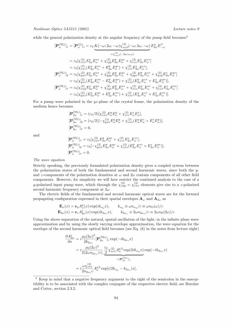
Nonlinear Optics 5A5513 (2003) Lecture notes 9
while the general polarization density at the angular frequency of the pump field becomes3
[P(NL)ω ]z = [P(2)
ω ]z = ε0K(−ω; 2ω,−ω)χ(2)zαβ(−ω; 2ω,−ω)
︸ ︷︷ ︸=χ
(2)
zαβ(−2ω;ω,ω)
Eα2ωEβ−ω
= ε0[χ(2)zxxE
x2ωE
x∗ω + χ(2)
zyyEy2ωE
y∗ω + χ(2)
zzzEz2ωE
z∗ω ]
= ε0[χ(2)zxx(E
x2ωE
x∗ω + Ey2ωE
y∗ω ) + χ(2)
zzzEz2ωE
z∗ω ],
[P(NL)ω ]y = ε0[χ
(2)yxxE
x2ωE
x∗ω + χ(2)
yyyEy2ωE
y∗ω + χ(2)
yyzEy2ωE
z∗ω + χ(2)
yzyEz2ωE
y∗ω ]
= ε0[χ(2)yxx(E
x2ωE
x∗ω − Ey2ωE
y∗ω ) + χ(2)
zxx(Ey2ωE
z∗ω + Ez2ωE
y∗ω )],
[P(NL)ω ]x = ε0[χ
(2)xxyE
x2ωE
y∗ω + χ(2)
xyxEy2ωE
x∗ω + χ(2)
xxzEx2ωE
z∗ω + χ(2)
xzxEz2ωE
x∗ω ]
= ε0[χ(2)yxx(E
x2ωE
y∗ω + Ey2ωE
x∗ω ) + χ(2)
zxx(Ex2ωE
z∗ω + Ez2ωE
x∗ω )].
For a pump wave polarized in the yz-plane of the crystal frame, the polarization density of themedium hence becomes
[P(NL)2ω ]z = (ε0/2)[χ
(2)zxxE
yωE
yω + χ(2)
zzzEzωE
zω],
[P(NL)2ω ]y = (ε0/2)[−χ(2)
yxxEyωE
yω + χ(2)
zxx(EyωE
zω + EzωE
yω)],
[P(NL)2ω ]x = 0,
and[P(NL)
ω ]z = ε0[χ(2)zxxE
y2ωE
y∗ω + χ(2)
zzzEz2ωE
z∗ω ],
[P(NL)ω ]y = ε0[−χ(2)
yxxEy2ωE
y∗ω + χ(2)
zxx(Ey2ωE
z∗ω + Ez2ωE
y∗ω )],
[P(NL)ω ]x = 0.
The wave equation
Strictly speaking, the previously formulated polarization density gives a coupled system betweenthe polarization states of both the fundamental and second harmonic waves, since both the y-and z-components of the polarization densities at ω and 2ω contain components of all other fieldcomponents. However, for simplicity we will here restrict the continued analysis to the case of a
y-polarized input pump wave, which through the χ(2)zyy = χ
(2)zxx elements give rise to a z-polarized
second harmonic frequency component at 2ω.The electric fields of the fundamental and second harmonic optical waves are for the forward
propagating configuration expressed in their spatial envelopes Aω and A2ω as
Eω(x) = eyAyω(x) exp(ikωy
x), kωy≡ ωnωy
/c ≡ ωnO(ω)/c
E2ω(x) = ezAz2ω(x) exp(ik2ωz
x), k2ωz≡ 2ωn2ωz
/c ≡ 2ωnE(2ω)/c
Using the above separation of the natural, spatial oscillation of the light, in the infinite plane waveapproximation and by using the slowly varying envelope approximation, the wave equation for theenvelope of the second harmonic optical field becomes (see Eq. (6) in the notes from lecture eight)
∂Az2ω∂x
= iµ0(2ω)2
2k2ωz
[P(NL)2ω ]z exp(−ik2ωz
x)
= iµ0(2ω)2
2(2ωn2ωz/c)
ε02χ(2)zxxA
yω
2 exp(2ikωyx)
︸ ︷︷ ︸=[P
(NL)2ω
]z
exp(−ik2ωzx)
= iωχ
(2)zxx
2n2ωzcAyω
2 exp[i(2kωy− k2ωz
)x],
3 Keep in mind that a negative frequency argument to the right of the semicolon in the suscep-tibility is to be associated with the complex conjugate of the respective electric field; see Butcherand Cotter, section 2.3.2.
94

Lecture notes 9 Nonlinear Optics 5A5513 (2003)
while for the fundamental wave,
∂Ayω∂x
= iµ0ω
2
2kωy
[P(NL)ω ]y exp(−ikωy
x)
= iµ0ω
2
2(ωnωy/c)
ε0χ(2)zxxA
z2ω exp(ik2ωz
x)Ay∗ω exp(−ikωyx)
︸ ︷︷ ︸=[P
(NL)ω ]y
exp(−ikωyx)
= iωχ
(2)zxx
2nωycAz2ωA
y∗ω exp[−i(2kωy
− k2ωz)x].
These equations can hence be summarized by the coupled system
∂Az2ω∂x
= iωχ
(2)zxx
2n2ωzcAyω
2 exp(i∆kx), (3a)
∂Ayω∂x
= iωχ
(2)zxx
2nωycAz2ωA
y∗ω exp(−i∆kx). (3b)
where∆k = 2kωy
− k2ωz
= 2ωnωy/c− 2ωn2ωz
/c
= (2ω/c)(nωy− ωn2ωz
)
is the so-called phase mismatch between the pump and second harmonic wave.
Boundary conditions
Here the boundary conditions are simply that no second harmonic signal is present at the input,
Az2ω(0) = 0,
together with a known input field at the fundamental frequency,
Ayω(0) = known.
Solving the wave equation
Considering a nonzero ∆k, the conversion efficiency is regularly quite small, and one may approx-imately take the spatial distribution of the pump wave to be constant, Ayω(x) ≈ Ayω(0). Using thisapproximation4, and by applying the initial condition Az2ω(0) = 0 of the second harmonic signal,one finds
Az2ω(L) =
∫ L
0
∂Az2ω(z)
∂xdx
=
∫ L
0
iωχ
(2)zxx
2n2ωzcAyω
2(0) exp(i∆kx) dx
=ωχ
(2)zxx
2n2ωzcAyω
2(0)1
∆k[exp(i∆kL) − 1]
=Use [exp(i∆kL) − 1]/∆k = iL exp(i∆kL/2) sinc(∆kL/2)
= iωχ
(2)zxxL
2n2ωzcAyω
2(0) exp(i∆kL/2) sinc(∆kL/2).
4 For an outline of the method of solving the coupled system (1) exactly in terms of Jacobianelliptic functions (thus allowing for a depleted pump as well), see J. A. Armstrong, N. Bloembergen,J. Ducuing, and P. S. Pershan, Phys. Rev. 127, 1918–1939, (1962).
95
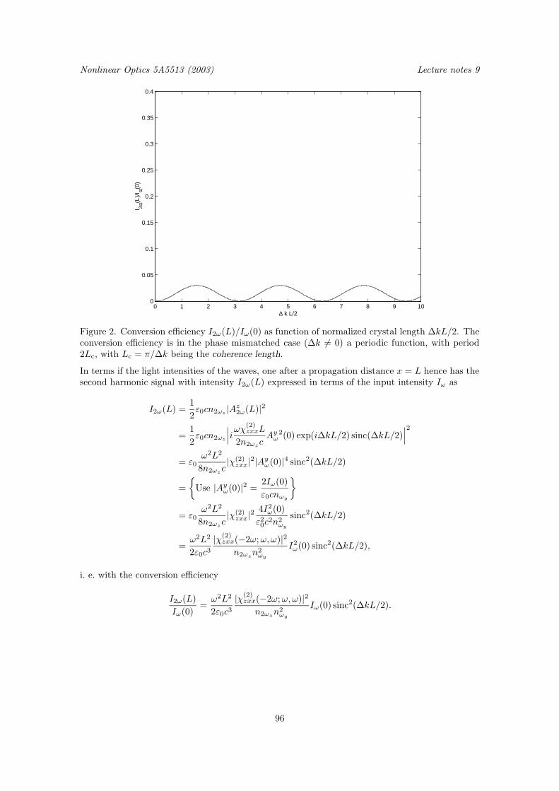
Nonlinear Optics 5A5513 (2003) Lecture notes 9
0 1 2 3 4 5 6 7 8 9 100
0.05
0.1
0.15
0.2
0.25
0.3
0.35
0.4
∆ k L/2
I 2ω(L
)/I ω
(0)
Figure 2. Conversion efficiency I2ω(L)/Iω(0) as function of normalized crystal length ∆kL/2. Theconversion efficiency is in the phase mismatched case (∆k 6= 0) a periodic function, with period2Lc, with Lc = π/∆k being the coherence length.
In terms if the light intensities of the waves, one after a propagation distance x = L hence has thesecond harmonic signal with intensity I2ω(L) expressed in terms of the input intensity Iω as
I2ω(L) =1
2ε0cn2ωz
|Az2ω(L)|2
=1
2ε0cn2ωz
∣∣∣iωχ(2)zxxL
2n2ωzcAyω
2(0) exp(i∆kL/2) sinc(∆kL/2)∣∣∣2
= ε0ω2L2
8n2ωzc|χ(2)zxx|2|Ayω(0)|4 sinc2(∆kL/2)
=
Use |Ayω(0)|2 =
2Iω(0)
ε0cnωy
= ε0ω2L2
8n2ωzc|χ(2)zxx|2
4I2ω(0)
ε20c2n2ωy
sinc2(∆kL/2)
=ω2L2
2ε0c3|χ(2)zxx(−2ω;ω, ω)|2n2ωz
n2ωy
I2ω(0) sinc2(∆kL/2),
i. e. with the conversion efficiency
I2ω(L)
Iω(0)=ω2L2
2ε0c3|χ(2)zxx(−2ω;ω, ω)|2n2ωz
n2ωy
Iω(0) sinc2(∆kL/2).
96

Lecture notes 9 Nonlinear Optics 5A5513 (2003)
0.5 1 1.51.5
1.52
1.54
1.56
1.58
1.6
1.62
vacuum wavelength
refr
activ
e in
dex
no, ordinary ray
ne, extraordinary ray
Figure 3. Ordinary and extraordinary refractive indices of a negative uniaxial crystal as functionof vacuum wavelength of the light, in the case of normal dispersion. Phase matching between thepump and second harmonic wave is obtained whenever nωy
≡ nO(ω) = nE(2ω) ≡ n2ωz.
0 1 2 3 4 5 6 7 8 9 100
0.05
0.1
0.15
0.2
0.25
0.3
0.35
0.4
∆ k L/2
I 2ω(L
)/I ω
(0)
Figure 4. Conversion efficiency I2ω(L)/Iω(0) as function of normalized crystal length ∆kL/2 whenthe material properties are periodically reversed, with a half-period of Lc.
97

Nonlinear Optics 5A5513 (2003) Lecture notes 9
Optical Kerr-effect - Field corrected refractive index
As a start, we assume a monochromatic optical wave (containing forward and/or backward prop-agating components) polarized in the xy-plane,
E(z, t) = Re[Eω(z) exp(−iωt)] ∈ R3,
with all spatial variation of the field contained in
Eω(z) = exExω(z) + eyE
yω(z) ∈ C
3.
The optical interaction
Optical Kerr-effect is in isotropic media described by the third order susceptibility5
χ(3)µαβγ(−ω;ω, ω,−ω).
Symmetries of the medium
The general set of nonzero components of χ(3)µαβγ for isotropic media are from Appendix A3.3 of
Butcher and Cotters book given as
χ(3)xxxx = χ(3)
yyyy = χ(3)zzzz ,
χ(3)yyzz = χ(3)
zzyy = χ(3)zzxx = χ(3)
xxzz = χ(3)xxyy = χ(3)
yyxx
χ(3)yzyz = χ(3)
zyzy = χ(3)zxzx = χ(3)
xzxz = χ(3)xyxy = χ(3)
yxyx
χ(3)yzzy = χ(3)
zyyz = χ(3)zxxz = χ(3)
xzzx = χ(3)xyyx = χ(3)
yxxy
(4)
withχ(3)xxxx = χ(3)
xxyy + χ(3)xyxy + χ(3)
xyyx,
i. e. a general set of 21 elements, of which only 3 are independent.
Additional symmetries
By applying the intrinsic permutation symmetry in the middle indices for optical Kerr-effect, onegenerally has
χ(3)µαβγ(−ω;ω, ω,−ω) = χ
(3)µβαγ(−ω;ω, ω,−ω),
which hence slightly reduce the set (4) to still 21 nonzero elements, but of which now only two areindependent. For a beam polarized in the xy-plane, the elements of interest are only those whichonly contain x or y in the indices, i. e. the subset
χ(3)xxxx = χ(3)
yyyy , χ(3)xxyy = χ(3)
yyxx =
intr. perm. symm.
(α, ω) (β, ω)
= χ(3)
xyxy = χ(3)yxyx, χ(3)
xyyx = χ(3)yxxy ,
withχ(3)xxxx = χ(3)
xxyy + χ(3)xyxy + χ(3)
xyyx,
i. e. a set of eight elements, of which only two are independent.
5 Again, keep in mind that in the convention of Butcher and Cotter, the frequency arguments tothe right of the semicolon may be writen in arbitrary order, hence we may in an equal descriptioninstead use
χ(3)µαβγ(−ω;ω,−ω, ω)
orχ
(3)µαβγ(−ω;−ω, ω, ω)
for this description of the third order interaction between light and matter.
98
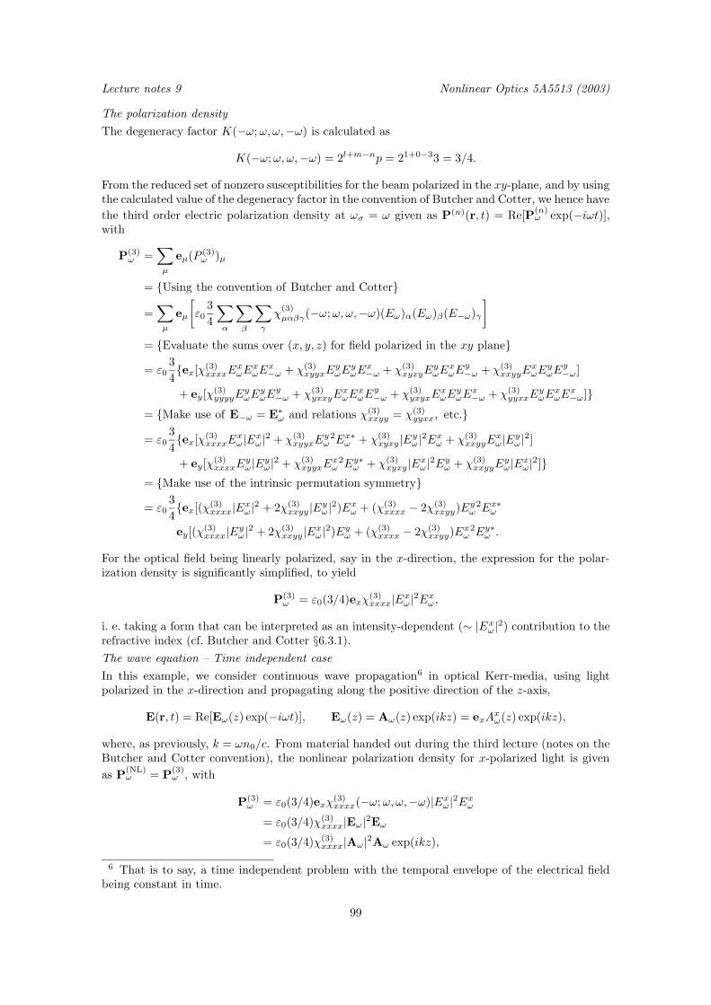
Lecture notes 9 Nonlinear Optics 5A5513 (2003)
The polarization density
The degeneracy factor K(−ω;ω, ω,−ω) is calculated as
K(−ω;ω, ω,−ω) = 2l+m−np = 21+0−33 = 3/4.
From the reduced set of nonzero susceptibilities for the beam polarized in the xy-plane, and by usingthe calculated value of the degeneracy factor in the convention of Butcher and Cotter, we hence have
the third order electric polarization density at ωσ = ω given as P(n)(r, t) = Re[P(n)ω exp(−iωt)],
with
P(3)ω =
∑
µ
eµ(P(3)ω )µ
= Using the convention of Butcher and Cotter
=∑
µ
eµ
[ε0
3
4
∑
α
∑
β
∑
γ
χ(3)µαβγ(−ω;ω, ω,−ω)(Eω)α(Eω)β(E−ω)γ
]
= Evaluate the sums over (x, y, z) for field polarized in the xy plane
= ε03
4ex[χ(3)
xxxxExωE
xωE
x−ω + χ(3)
xyyxEyωE
yωE
x−ω + χ(3)
xyxyEyωE
xωE
y−ω + χ(3)
xxyyExωE
yωE
y−ω]
+ ey[χ(3)yyyyE
yωE
yωE
y−ω + χ(3)
yxxyExωE
xωE
y−ω + χ(3)
yxyxExωE
yωE
x−ω + χ(3)
yyxxEyωE
xωE
x−ω]
= Make use of E−ω = E∗ω and relations χ(3)
xxyy = χ(3)yyxx, etc.
= ε03
4ex[χ(3)
xxxxExω|Exω|2 + χ(3)
xyyxEyω
2Ex∗ω + χ(3)xyxy |Eyω|2Exω + χ(3)
xxyyExω|Eyω|2]
+ ey[χ(3)xxxxE
yω|Eyω|2 + χ(3)
xyyxExω
2Ey∗ω + χ(3)xyxy |Exω|2Eyω + χ(3)
xxyyEyω|Exω|2]
= Make use of the intrinsic permutation symmetry
= ε03
4ex[(χ(3)
xxxx|Exω|2 + 2χ(3)xxyy |Eyω|2)Exω + (χ(3)
xxxx − 2χ(3)xxyy)E
yω
2Ex∗ω
ey[(χ(3)xxxx|Eyω|2 + 2χ(3)
xxyy |Exω|2)Eyω + (χ(3)xxxx − 2χ(3)
xxyy)Exω
2Ey∗ω .
For the optical field being linearly polarized, say in the x-direction, the expression for the polar-ization density is significantly simplified, to yield
P(3)ω = ε0(3/4)exχ
(3)xxxx|Exω|2Exω,
i. e. taking a form that can be interpreted as an intensity-dependent (∼ |Exω|2) contribution to the
refractive index (cf. Butcher and Cotter §6.3.1).The wave equation – Time independent case
In this example, we consider continuous wave propagation6 in optical Kerr-media, using lightpolarized in the x-direction and propagating along the positive direction of the z-axis,
E(r, t) = Re[Eω(z) exp(−iωt)], Eω(z) = Aω(z) exp(ikz) = exAxω(z) exp(ikz),
where, as previously, k = ωn0/c. From material handed out during the third lecture (notes on theButcher and Cotter convention), the nonlinear polarization density for x-polarized light is given
as P(NL)ω = P
(3)ω , with
P(3)ω = ε0(3/4)exχ
(3)xxxx(−ω;ω, ω,−ω)|Exω|2Exω
= ε0(3/4)χ(3)xxxx|Eω|2Eω
= ε0(3/4)χ(3)xxxx|Aω|2Aω exp(ikz),
6 That is to say, a time independent problem with the temporal envelope of the electrical fieldbeing constant in time.
99

Nonlinear Optics 5A5513 (2003) Lecture notes 9
and the time independent wave equation for the field envelope Aω, using Eq. (6), becomes
∂
∂zAω = i
µ0ω2
2kε0(3/4)χ
(3)xxxx|Aω|2Aω exp(ikz)︸ ︷︷ ︸
=P(NL)ω (z)
exp(−ikz)
= i3ω2
8c2kχ(3)xxxx|Aω|2Aω
= since k = ωn0(ω)/c
= i3ω
8cn0χ(3)xxxx|Aω|2Aω,
or, equivalently, in its scalar form
∂
∂zAxω = i
3ω
8cn0χ(3)xxxx|Axω|2Axω.
Boundary conditions – Time independent case
For this special case of unidirectional wave propagation, the boundary condition is simply a knownoptical field at the input,
Axω(0) = known.
Solving the wave equation – Time independent case
If the medium of interest now is analyzed at an angular frequency far from any resonance, we maylook for solutions to this equation with |Aω(z)| being constant (for a lossless medium). For sucha case it is straightforward to integrate the final wave equation to yield the general solution
Aω(z) = Aω(0) exp[i3ω
8cn0χ(3)xxxx|Aω(0)|2z],
or, again equivalently, in the scalar form
Axω(z) = Axω(0) exp[i3ω
8cn0χ(3)xxxx|Axω(0)|2z],
which hence gives the solution for the real-valued electric field E(r, t) as
E(r, t) = Re[Eω(z) exp(−iωt)]= ReAω(z) exp[i(kz − ωt)]
= ReAω(0) exp[i(ωn0
cz +
3ω
8cn0χ(3)xxxx|Axω(0)|2z
︸ ︷︷ ︸≡keffz
−ωt)].
From this solution, one immediately finds that the wave propagates with an effective propagationconstant
keff =ω
c[n0 +
3
8n0χ(3)xxxx|Axω(0)|2],
that is to say, experiencing the intensity dependent refractive index
neff = n0 +3
8n0χ(3)xxxx|Axω(0)|2
= n0 + n2|Axω(0)|2,
with
n2 =3
8n0χ(3)xxxx.
100
Lecture Notes on Nonlinear Optics Nonlinear Optics 5A5513 (2003)
Lecture X
101

Nonlinear Optics 5A5513 (2003) Lecture Notes on Nonlinear Optics
Lecture Notes on Nonlinear OpticsNonlinear Optics (5A5513, 5p for advanced undergraduate and doctoral students)Course given at the Royal Institute of Technology,Department of Laser Physics and Quantum OpticsSE–106 91, Stockholm, SwedenJanuary 8 – March 24, 2003
The texts and figures in this lecture series was typeset by the author in 10/12/16 pt ComputerModern typeface using plain TEX and METAPOST.
This document is electronically available at the homepage of the Library of the Royal Institute ofTechnology, at http://www.lib.kth.se.
Copyright c© Fredrik Jonsson 2003
All rights reserved. No part of this publication may be reproduced, stored in a retrieval system,or transmitted, in any form, or by any means, electronic, mechanical, photo-copying, recording, orotherwise, without the prior consent of the author.
ISBN 91-7283-517-6TRITA-FYS 2003:26ISSN 0280-316XISRN KTH/FYS/- - 03:26 - - SEPrinted on July 7, 2003
TEX is a trademark of the American Mathematical Society
102

Nonlinear Optics 5A5513 (2003)Lecture notes
Lecture 10
In this lecture, we will focus on examples of electromagnetic wave propagation in nonlinear opticalmedia, by applying the forms of Maxwell’s equations as obtained in the eighth lecture to a set ofparticular nonlinear interactions as described by the previously formulated nonlinear susceptibilityformalism.
The outline for this lecture is:• What are solitons?• Basics of soliton theory• Spatial and temporal solitons• The mathematical equivalence between spatial and temporal solitons• The creation of temporal and spatial solitons
What are solitons?
The first reported observation of solitons was made in 1834 by John Scott Russell, a Scottishscientist and later famous Victorian engineer and shipbuilder, while studying water waves in theGlasgow-Edinburgh channel. As part of this investigation, he was observing a boat being pulledalong, rapidly, by a pair of horses. For some reason, the horses stopped the boat rather suddenly,and the stopping of the boat caused a verystrong wave to be generated. This wave, in fact, asignificant hump of water stretching across the rather narrow canal, rose up at the front of theboat and proceeded to travel, quite rapidly down the canal. Russell, immediately, realised thatthe wave was something very special. It was “alone”, in the sense that it sat on the canal with nodisturbance to the front or the rear, nor did it die away until he had followed it for quite a longway. The word “alone” is synonymous with “solitary”, and Russell soon referred to his observationas the Great Solitary Wave.
The word “solitary” is now routinely used, indeed even the word “solitary” tends to be re-placed by the more generic word “soliton”. Once the physics behind Russell’s wave is understood,however, solitons, of one kind or another, appear to be everywhere but it is interesting that theunderlying causes of soliton generation were not understood by Russell, and only partially by hiscontemporaries.
Classes of solitons
Bright temporal envelope solitons
Pulses of light with a certain shape and energy that can propagate unchanged over large distances.This is the class of solitons which we will focus on in this lecture.
Dark temporal envelope solitons
Pulses of “darkness” within a continuous wave, where the pulses are of a certain shape, and possesspropagation properties similar to the bright solitons.
Spatial solitons
Continuous wave beams or pulses, with a transverse extent of the beam that via the refractive indexchange due to optical Kerr-effect can compensate for the diffraction of the beam. The opticallyinduced change of refractive index works as an effective waveguide for the light.
103
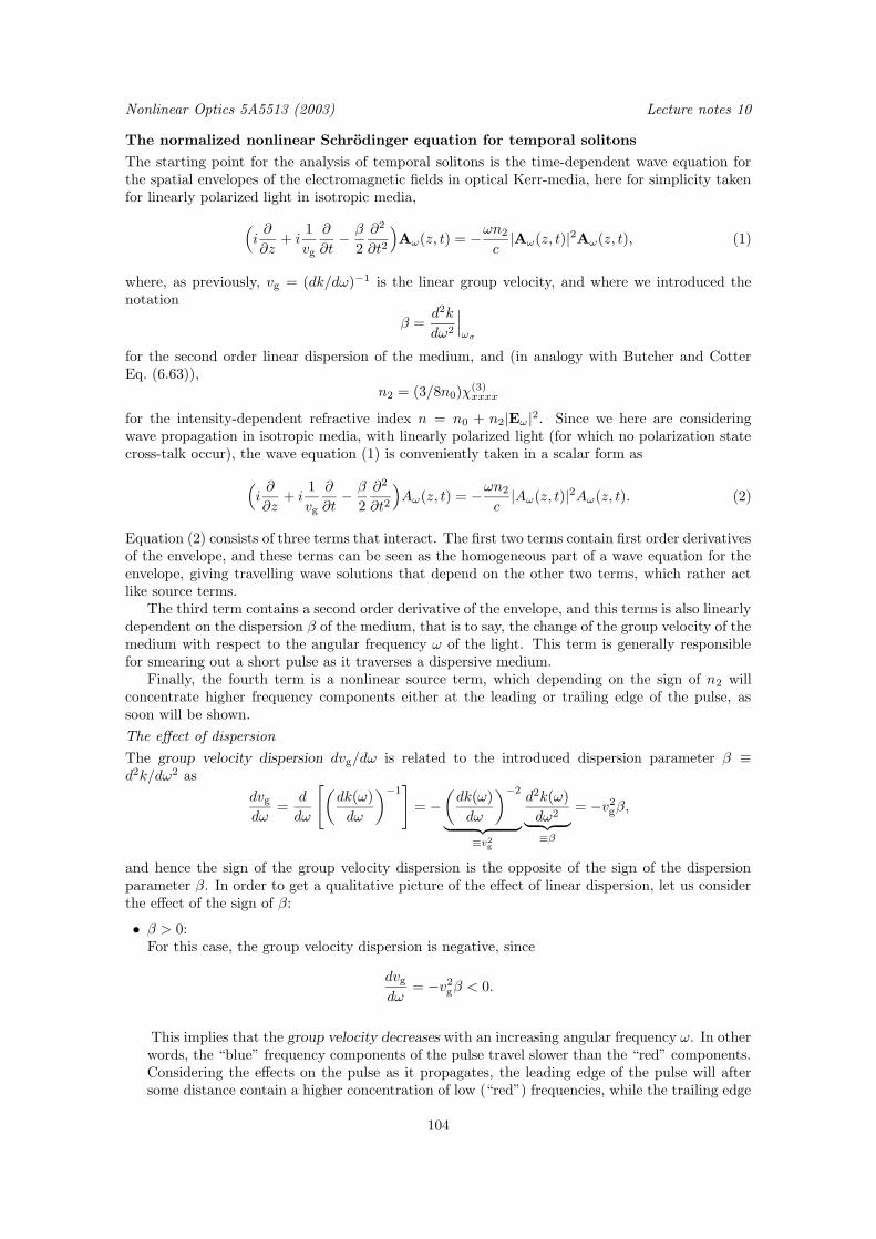
Nonlinear Optics 5A5513 (2003) Lecture notes 10
The normalized nonlinear Schrodinger equation for temporal solitons
The starting point for the analysis of temporal solitons is the time-dependent wave equation forthe spatial envelopes of the electromagnetic fields in optical Kerr-media, here for simplicity takenfor linearly polarized light in isotropic media,
(i∂
∂z+ i
1
vg
∂
∂t− β
2
∂2
∂t2
)Aω(z, t) = −ωn2
c|Aω(z, t)|2Aω(z, t), (1)
where, as previously, vg = (dk/dω)−1 is the linear group velocity, and where we introduced thenotation
β =d2k
dω2
∣∣∣ωσ
for the second order linear dispersion of the medium, and (in analogy with Butcher and CotterEq. (6.63)),
n2 = (3/8n0)χ(3)xxxx
for the intensity-dependent refractive index n = n0 + n2|Eω|2. Since we here are consideringwave propagation in isotropic media, with linearly polarized light (for which no polarization statecross-talk occur), the wave equation (1) is conveniently taken in a scalar form as
(i∂
∂z+ i
1
vg
∂
∂t− β
2
∂2
∂t2
)Aω(z, t) = −ωn2
c|Aω(z, t)|2Aω(z, t). (2)
Equation (2) consists of three terms that interact. The first two terms contain first order derivativesof the envelope, and these terms can be seen as the homogeneous part of a wave equation for theenvelope, giving travelling wave solutions that depend on the other two terms, which rather actlike source terms.
The third term contains a second order derivative of the envelope, and this terms is also linearlydependent on the dispersion β of the medium, that is to say, the change of the group velocity of themedium with respect to the angular frequency ω of the light. This term is generally responsiblefor smearing out a short pulse as it traverses a dispersive medium.
Finally, the fourth term is a nonlinear source term, which depending on the sign of n2 willconcentrate higher frequency components either at the leading or trailing edge of the pulse, assoon will be shown.
The effect of dispersion
The group velocity dispersion dvg/dω is related to the introduced dispersion parameter β ≡d2k/dω2 as
dvgdω
=d
dω
[(dk(ω)
dω
)−1]
= −(dk(ω)
dω
)−2
︸ ︷︷ ︸≡v2g
d2k(ω)
dω2︸ ︷︷ ︸≡β
= −v2gβ,
and hence the sign of the group velocity dispersion is the opposite of the sign of the dispersionparameter β. In order to get a qualitative picture of the effect of linear dispersion, let us considerthe effect of the sign of β:
• β > 0:For this case, the group velocity dispersion is negative, since
dvgdω
= −v2gβ < 0.
This implies that the group velocity decreases with an increasing angular frequency ω. In otherwords, the “blue” frequency components of the pulse travel slower than the “red” components.Considering the effects on the pulse as it propagates, the leading edge of the pulse will aftersome distance contain a higher concentration of low (“red”) frequencies, while the trailing edge
104
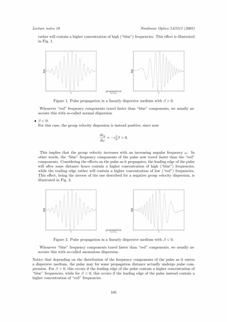
Lecture notes 10 Nonlinear Optics 5A5513 (2003)
rather will contain a higher concentration of high (“blue”) frequencies. This effect is illustratedin Fig. 1.
t
E(t
)
propagation7−→ t
E(t
)
Figure 1. Pulse propagation in a linearly dispersive medium with β > 0.
Whenever “red” frequency components travel faster than “blue” components, we usually as-sociate this with so-called normal dispersion.
• β < 0:For this case, the group velocity dispersion is instead positive, since now
dvgdω
= −v2gβ > 0.
This implies that the group velocity increases with an increasing angular frequency ω. Inother words, the “blue” frequency components of the pulse now travel faster than the “red”components. Considering the effects on the pulse as it propagates, the leading edge of the pulsewill after some distance hence contain a higher concentration of high (“blue”) frequencies,while the trailing edge rather will contain a higher concentration of low (“red”) frequencies.This effect, being the inverse of the one described for a negative group velocity dispersion, isillustrated in Fig. 2.
t
E(t
)
propagation7−→ t
E(t
)
Figure 2. Pulse propagation in a linearly dispersive medium with β < 0.
Whenever “blue” frequency components travel faster than “red” components, we usually as-sociate this with so-called anomalous dispersion.
Notice that depending on the distribution of the frequency components of the pulse as it entersa dispersive medium, the pulse may for some propagation distance actually undergo pulse com-pression. For β > 0, this occurs if the leading edge of the pulse contain a higher concentration of“blue” frequencies, while for β < 0, this occurs if the leading edge of the pulse instead contain ahigher concentration of “red” frequencies.
105
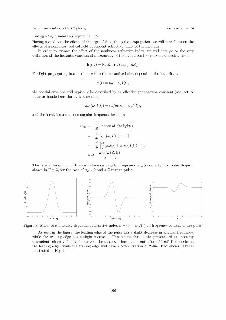
Nonlinear Optics 5A5513 (2003) Lecture notes 10
The effect of a nonlinear refractive index
Having sorted out the effects of the sign of β on the pulse propagation, we will now focus on theeffects of a nonlinear, optical field dependent refractive index of the medium.
In order to extract the effect of the nonlinear refractive index, we will here go to the verydefinition of the instantaneous angular frequency of the light from its real-valued electric field,
E(r, t) = Re[Eω(r, t) exp(−iωt)].
For light propagating in a medium where the refractive index depend on the intensity as
n(t) = n0 + n2I(t),
the spatial envelope will typically be described by an effective propagation constant (see lecturenotes as handed out during lecture nine)
keff(ω, I(t)) = (ω/c)(n0 + n2I(t)),
and the local, instantaneous angular frequency becomes
ωloc = − d
dt
phase of the light
= − d
dt[keff(ω, I(t)) − ωt]
= − d
dt
[ωc(n0(ω) + n2(ω)I(t))
]+ ω
= ω − ωn2(ω)
c
dI(t)
dt.
The typical behaviour of the instantaneous angular frequancy ωloc(t) on a typical pulse shape isshown in Fig. 3, for the case of n2 > 0 and a Gaussian pulse.
−10 −8 −6 −4 −2 0 2 4 6 8 10
0
0.2
0.4
0.6
0.8
1
t [arb. units]
I(t)
[arb
. uni
ts]
−10 −8 −6 −4 −2 0 2 4 6 8 10
−0.5
−0.4
−0.3
−0.2
−0.1
0
0.1
0.2
0.3
0.4
0.5
t [arb. units]
dI(t
)/dt
[arb
. uni
ts]
−10 −8 −6 −4 −2 0 2 4 6 8 100
0.5
1
1.5
2
2.5
3
3.5
4
t
ω lo
c(t)=
ω−
(n2ω
/c)d
I(t)
/dt
Figure 3. Effect of a intensity dependent refractive index n = n0 + n2I(t) on frequency content of the pulse.
As seen in the figure, the leading edge of the pulse has a slight decrease in angular frequency,while the trailing edge has a slight increase. This means that in the presence of an intensitydependent refractive index, for n2 > 0, the pulse will have a concentration of “red” frequencies atthe leading edge, while the trailing edge will have a concentration of “blue” frequencies. This isillustrated in Fig. 4.
106
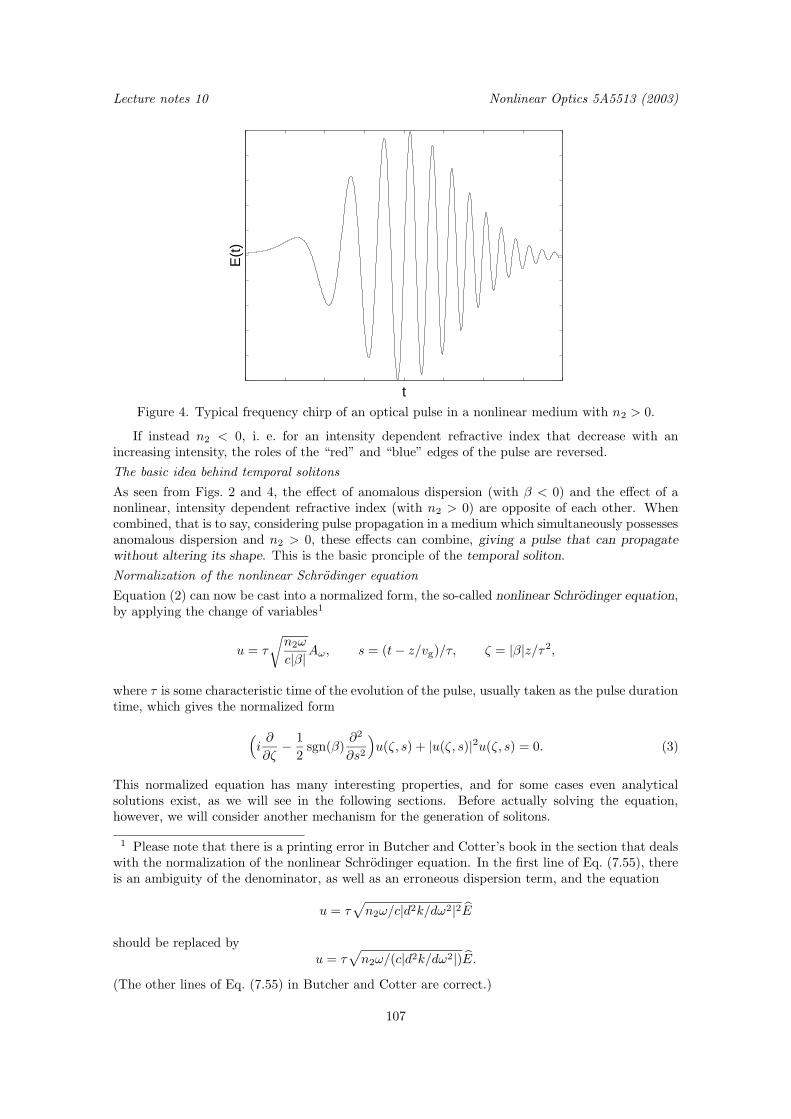
Lecture notes 10 Nonlinear Optics 5A5513 (2003)
t
E(t
)
Figure 4. Typical frequency chirp of an optical pulse in a nonlinear medium with n2 > 0.
If instead n2 < 0, i. e. for an intensity dependent refractive index that decrease with anincreasing intensity, the roles of the “red” and “blue” edges of the pulse are reversed.
The basic idea behind temporal solitons
As seen from Figs. 2 and 4, the effect of anomalous dispersion (with β < 0) and the effect of anonlinear, intensity dependent refractive index (with n2 > 0) are opposite of each other. Whencombined, that is to say, considering pulse propagation in a medium which simultaneously possessesanomalous dispersion and n2 > 0, these effects can combine, giving a pulse that can propagatewithout altering its shape. This is the basic pronciple of the temporal soliton.
Normalization of the nonlinear Schrodinger equation
Equation (2) can now be cast into a normalized form, the so-called nonlinear Schrodinger equation,by applying the change of variables1
u = τ
√n2ω
c|β|Aω, s = (t− z/vg)/τ, ζ = |β|z/τ 2,
where τ is some characteristic time of the evolution of the pulse, usually taken as the pulse durationtime, which gives the normalized form
(i∂
∂ζ− 1
2sgn(β)
∂2
∂s2
)u(ζ, s) + |u(ζ, s)|2u(ζ, s) = 0. (3)
This normalized equation has many interesting properties, and for some cases even analyticalsolutions exist, as we will see in the following sections. Before actually solving the equation,however, we will consider another mechanism for the generation of solitons.
1 Please note that there is a printing error in Butcher and Cotter’s book in the section that dealswith the normalization of the nonlinear Schrodinger equation. In the first line of Eq. (7.55), thereis an ambiguity of the denominator, as well as an erroneous dispersion term, and the equation
u = τ√n2ω/c|d2k/dω2|2E
should be replaced byu = τ
√n2ω/(c|d2k/dω2|)E.
(The other lines of Eq. (7.55) in Butcher and Cotter are correct.)
107

Nonlinear Optics 5A5513 (2003) Lecture notes 10
Before leaving the temporal pulse propagation, a few remarks on the signs of the dispersionterm β and the nonlinear refractive index n2 should be made. Whenever β > 0, the group velocitydispersion
dvgdω
≡ d
dω
[(dk
dω
)−1]
= −(dk
dω
)−2d2k
dω2= −v2
g
d2k
dω2
will be negative, and the pulse will experience what we call a normal dispersion, for which therefractive index of the medium decrease with an increasing wavelength of the light. This is the“common” way dispersion enters in optical processes, where the pulse is broadened as it traversesthe medium.
Spatial solitons
As a light beam with some limited spatial extent in the transverse direction enter an optical Kerrmedia, the intensity variation across the beam will via the intensity dependent refractive indexn = n0 +n2I form a lensing through the medium. Depending on the sign of the coefficient n2 (the“nonlinear refractive index”), the beam will either experience a defocusing lensing effect (if n2 < 0)or a focusing lensing effect (if n2 > 0); in the latter case the beam itself will create a self-inducedwaveguide in the medium (see Fig. 5).
Optical Kerr-medium
Lfoc
(Self-trapping may occur)
k
x
I(x)
Figure 5. An illustration of the effect of self-focusing.
As being the most important case for beams with maximum intensity in the middle of the beam(as we usually encounter them in most situations), we will focus on the case n2 > 0. For this case,highly intense beams may cause such a strong focusing that the beam eventually break up again,due to strong diffraction effects for very narrow beams, or even due to material damage in thenonlinear crystal.
For some situations, however, there exist stationary solutions to the spatial light distributionthat exactly balance between the self-focusing and the diffraction of the beam. We can picture thisas a balance between two lensing effects, with the first one due to self-focusing, with an effectivefocal length ffoc (see Fig. 6), and the second one due to diffraction, with an effective focal lengthof fdefoc (see Fig. 7).
108
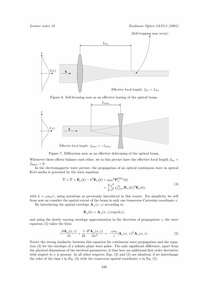
Lecture notes 10 Nonlinear Optics 5A5513 (2003)
Lfoc
(Self-trapping may occur)
k
Effective focal length: ffoc = Lfoc
x
I(x)
Figure 6. Self-focusing seen as an effective lensing of the optical beam.
Ldefoc
k
Effective focal length: fdefoc = −Ldefoc
x
I(x)
Figure 7. Diffraction seen as an effective defocusing of the optical beam.
Whenever these effects balance each other, we in this picture have the effective focal length ffoc +fdefoc = 0.
In the electromagnetic wave picture, the propagation of an optical continuous wave in opticalKerr-media is governed by the wave equation
∇×∇× Eω(r) − k2Eω(r) = µ0ω2P(NL)
ω (r)
=3
4
ω2
c2χ(3)xxxx|Eω(r)|2Eω(r),
(4)
with k = ωn0/c, using notations as previously introduced in this course. For simplicity we willfrom now on consider the spatial extent of the beam in only one transverse Cartesian coordinate x.
By introducing the spatial envelope Aω(x, z) according to
Eω(r) = Aω(x, z) exp(ikz),
and using the slowly varying envelope approximation in the direction of propagation z, the waveequation (4) takes the form
i∂Aω(x, z)
∂z+
1
2k
∂2Aω(x, z)
∂x2= −ωn2
c|Aω(x, z)|2Aω(x, z). (5)
Notice the strong similarity between this equation for continuous wave propagation and the equa-tion (3) for the envelope of a infinite plane wave pulse. The only significant difference, apart fromthe physical dimensions of the involved parameters, is that here nu additional first order derivativewith respect to x is present. In all other respects, Eqs. (3) and (5) are identical, if we interchangethe roles of the time t in Eq. (3) with the transverse spatial coordinate x in Eq. (5).
109

Nonlinear Optics 5A5513 (2003) Lecture notes 10
While the sign of the dispersion parameter β occurring in Eq. (3) has significance for the com-pression or broadening of the pulse, no such sign option appear in Eq. (5) for the spatial envelope ofthe continuous wave beam. This follows naturally, since the spatial broadening mechanism (in con-trary to the temporal compression or broadening of the pulse) is due to diffraction, a non-reversibleprocess which in nature always tend to broaden a collimated light beam.
As with Eq. (3) for the temporal pulse propagation, we may now for the continuous wave casecast Eq. (5) into a normalized form, by applying the change of variables
u = L
√n2ωk
cAω, s = x/L, ζ = z/(kL2),
where L is some characteristic length of the evolution of the beam, usually taken as the transversebeam width, which gives the normalized form
(i∂
∂ζ+
1
2
∂2
∂s2
)u(ζ, s) + |u(ζ, s)|2u(ζ, s) = 0. (6)
Mathematical equivalence between temporal and spatial solitons
As seen in the above derivation of the normalized forms of the equations governing wave propagationof temporal and spatial solitons, they are described by exactly the same normalized nonlinearSchrodinger equation. The only difference between the two cases are the ways the normalizationis being carried out. In the interpretation of the solutions to the nonlinear Schrodinger equation,the s variable could for the temporal solitons be taken as a normalized time variable, while for thespatial solitons, the s variable could instead be taken as a normalized transverse coordinate.
Soliton solutions
The nonlinear Schrodinger equations given by Eqs. (3) and (6) possess infinitely many solutions,of which only a few are possible to obtain analytically. In the regime where dvg/dω > 0 (i. e. forwhich β < 0), an exact temporal soliton solution to Eq. (3) is though obtained when the pulseu(ζ, s) has the initial shape
u(0, s) = N sech(s),
where N ≥ 1 is an integer number. Depending on the value of N , solitons of different order can beformed, and the so-called “fundamental soliton” is given for N = 1. For higher values of N , thesolitons are hence called “higher order solitons”.
The first analytical solution to the nonlinear Schrodinger equation is given for N = 1 as2
u(ζ, s) = sech(s) exp(iζ/2).
The shape of this fundamental solution is shown in Fig. 8.
2 Please note that there is a printing error in Butcher and Cotter’s The Elements of NonlinearOptics in their expression for this solution, on page 241, row 30, where their erroneous equation“u(ζ, s) = sech(s) exp(−iζ/2)” should be replaced by the proper one, without the minus sign inthe exponential.
110
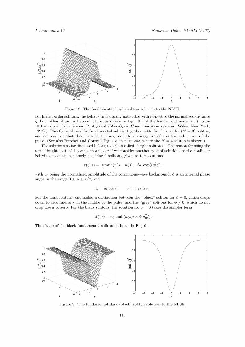
Lecture notes 10 Nonlinear Optics 5A5513 (2003)
−4−2
02
4
0
5
100
0.2
0.4
0.6
0.8
1
sζ
|u(ζ
,s)|
2
−4 −3 −2 −1 0 1 2 3 40
0.2
0.4
0.6
0.8
1
s
|u(ζ
,s)|
2
Figure 8. The fundamental bright soliton solution to the NLSE.
For higher order solitons, the behaviour is usually not stable with respect to the normalized distanceζ, but rather of an oscillatory nature, as shown in Fig. 10.1 of the handed out material. (Figure10.1 is copied from Govind P. Agrawal Fiber-Optic Communication systems (Wiley, New York,1997).) This figure shows the fundamental soliton together with the third order (N = 3) soliton,and one can see that there is a continuous, oscillatory energy transfer in the s-direction of thepulse. (See also Butcher and Cotter’s Fig. 7.8 on page 242, where the N = 4 soliton is shown.)
The solutions so far discussed belong to a class called “bright solitons”. The reason for using theterm “bright soliton” becomes more clear if we consider another type of solutions to the nonlinearSchrdinger equation, namely the “dark” solitons, given as the solutions
u(ζ, s) = [η tanh(η(s− κζ)) − iκ] exp(iu20ζ),
with u0 being the normalized amplitude of the continuous-wave background, φ is an internal phaseangle in the range 0 ≤ φ ≤ π/2, and
η = u0 cosφ, κ = u0 sinφ.
For the dark solitons, one makes a distinction between the “black” soliton for φ = 0, which dropsdown to zero intensity in the middle of the pulse, and the “grey” solitons for φ 6= 0, which do notdrop down to zero. For the black solitons, the solution for φ = 0 takes ths simpler form
u(ζ, s) = u0 tanh(u0s) exp(iu20ζ).
The shape of the black fundamental soliton is shown in Fig. 9.
−4−2
02
4
0
5
100
0.2
0.4
0.6
0.8
1
sζ
|u(ζ
,s)|
2
−4 −3 −2 −1 0 1 2 3 40
0.2
0.4
0.6
0.8
1
s
|u(ζ
,s)|
2
Figure 9. The fundamental dark (black) soliton solution to the NLSE.
111
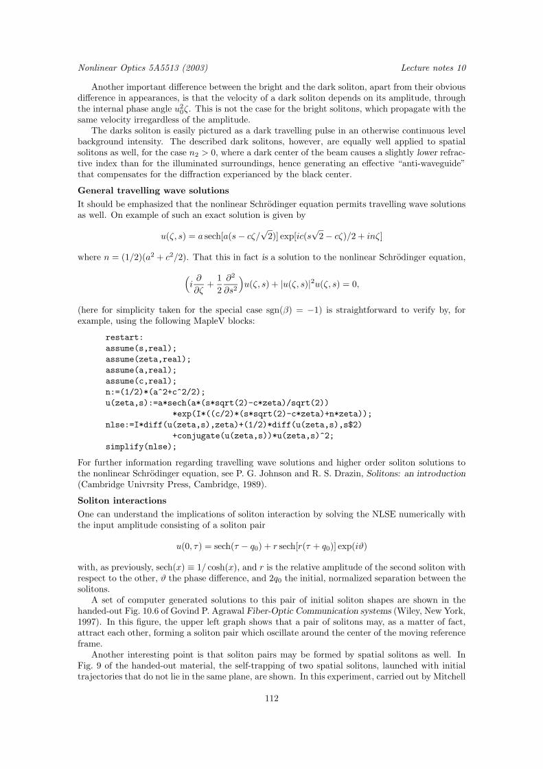
Nonlinear Optics 5A5513 (2003) Lecture notes 10
Another important difference between the bright and the dark soliton, apart from their obviousdifference in appearances, is that the velocity of a dark soliton depends on its amplitude, throughthe internal phase angle u2
0ζ. This is not the case for the bright solitons, which propagate with thesame velocity irregardless of the amplitude.
The darks soliton is easily pictured as a dark travelling pulse in an otherwise continuous levelbackground intensity. The described dark solitons, however, are equally well applied to spatialsolitons as well, for the case n2 > 0, where a dark center of the beam causes a slightly lower refrac-tive index than for the illuminated surroundings, hence generating an effective “anti-waveguide”that compensates for the diffraction experianced by the black center.
General travelling wave solutions
It should be emphasized that the nonlinear Schrodinger equation permits travelling wave solutionsas well. On example of such an exact solution is given by
u(ζ, s) = a sech[a(s− cζ/√
2)] exp[ic(s√
2 − cζ)/2 + inζ]
where n = (1/2)(a2 + c2/2). That this in fact is a solution to the nonlinear Schrodinger equation,
(i∂
∂ζ+
1
2
∂2
∂s2
)u(ζ, s) + |u(ζ, s)|2u(ζ, s) = 0,
(here for simplicity taken for the special case sgn(β) = −1) is straightforward to verify by, forexample, using the following MapleV blocks:
restart:
assume(s,real);
assume(zeta,real);
assume(a,real);
assume(c,real);
n:=(1/2)*(a^2+c^2/2);
u(zeta,s):=a*sech(a*(s*sqrt(2)-c*zeta)/sqrt(2))
*exp(I*((c/2)*(s*sqrt(2)-c*zeta)+n*zeta));
nlse:=I*diff(u(zeta,s),zeta)+(1/2)*diff(u(zeta,s),s$2)
+conjugate(u(zeta,s))*u(zeta,s)^2;
simplify(nlse);
For further information regarding travelling wave solutions and higher order soliton solutions tothe nonlinear Schrodinger equation, see P. G. Johnson and R. S. Drazin, Solitons: an introduction(Cambridge Univrsity Press, Cambridge, 1989).
Soliton interactions
One can understand the implications of soliton interaction by solving the NLSE numerically withthe input amplitude consisting of a soliton pair
u(0, τ) = sech(τ − q0) + r sech[r(τ + q0)] exp(iϑ)
with, as previously, sech(x) ≡ 1/ cosh(x), and r is the relative amplitude of the second soliton withrespect to the other, ϑ the phase difference, and 2q0 the initial, normalized separation between thesolitons.
A set of computer generated solutions to this pair of initial soliton shapes are shown in thehanded-out Fig. 10.6 of Govind P. Agrawal Fiber-Optic Communication systems (Wiley, New York,1997). In this figure, the upper left graph shows that a pair of solitons may, as a matter of fact,attract each other, forming a soliton pair which oscillate around the center of the moving referenceframe.
Another interesting point is that soliton pairs may be formed by spatial solitons as well. InFig. 9 of the handed-out material, the self-trapping of two spatial solitons, launched with initialtrajectories that do not lie in the same plane, are shown. In this experiment, carried out by Mitchell
112

Lecture notes 10 Nonlinear Optics 5A5513 (2003)
et. al. at Princeton3, the two solitons start spiraling around each other in a helix, experiencingattractive forces that together with the orbital momentum carried by the pulses form a stableconfiguration.
Dependence on initial conditions
For a real situation, one might ask oneself how sensitive the forming of solitons is, depending onperturbations on the preferred sech(s) initial shape. In a real situation, for example, we will rarelybe able to construct the exact pulse form required for launching a pulse that will possess the solitonproperties already from the beginning.
As a matter of fact, the soliton formation process accepts quite a broad range of initial pulseshapes, and as long as the initial intensity is sufficiently well matched to the energy content ofthe propagating soliton, the generated soliton is remarkable stable against perurbations. In afunctional theoretical analogy, we may call this the soliton “acceptance angle” of initial functionsthat will be accepted for soliton formation in a medium.
In order to illustrate the soliton formation, one may study Figs. 10.2 and 10.3 of GovindP. Agrawal Fiber-Optic Communication systems (Wiley, New York, 1997)4 In Fig. 10.2, the inputpulse shape is a Gaussian, rather than the natural sech(s) initial shape. As can be seen in the figure,the pulse shape gradually change towards the fundamental soliton, even though the Gaussian shapeis a quite bad approximation to the final sech(s) form.
The forming of the soliton does not only depend on the initial shape of the pulse, but alsoon the peak intensity of the pulse. In Fig. 10.3, an ideal sech(s) pulse shape, though with a 20percent higher pulse amplitude than the ideal one of unity, is used as input. In this case the pulseslightly oscillate in amplitude during the propagation, but finally approaching the fundamentalsoliton solution.
Finally, as being an example of an even worse approximation to the sech(s) shape, a squareinput pulse can also generate solitons, as shown in the handed-out Fig. 16 of Beam Shaping andControl with Nonlinear Optics, Eds. F. Kajzar and R. Reinisch (Plenum Press, New York, 1998).
3 M. Mitchell, Z. Chen, M. Shih, and M. Sageev, Phys. Rev. Lett. 77, 490 (1996).4 The same pictures can be found in Govind P. Agrawal Nonlinear Fiber Optics (Academic Press,
New York, 1989).
113

Nonlinear Optics 5A5513 (2003) Lecture notes 10
114

Lecture Notes on Nonlinear Optics Nonlinear Optics 5A5513 (2003)
Lecture XI
115

Nonlinear Optics 5A5513 (2003) Lecture Notes on Nonlinear Optics
Lecture Notes on Nonlinear OpticsNonlinear Optics (5A5513, 5p for advanced undergraduate and doctoral students)Course given at the Royal Institute of Technology,Department of Laser Physics and Quantum OpticsSE–106 91, Stockholm, SwedenJanuary 8 – March 24, 2003
The texts and figures in this lecture series was typeset by the author in 10/12/16 pt ComputerModern typeface using plain TEX and METAPOST.
This document is electronically available at the homepage of the Library of the Royal Institute ofTechnology, at http://www.lib.kth.se.
Copyright c© Fredrik Jonsson 2003
All rights reserved. No part of this publication may be reproduced, stored in a retrieval system,or transmitted, in any form, or by any means, electronic, mechanical, photo-copying, recording, orotherwise, without the prior consent of the author.
ISBN 91-7283-517-6TRITA-FYS 2003:26ISSN 0280-316XISRN KTH/FYS/- - 03:26 - - SEPrinted on July 7, 2003
TEX is a trademark of the American Mathematical Society
116

Nonlinear Optics 5A5513 (2003)Lecture notes
Lecture 11
In this lecture, we will focus on configurations where the angular frequency of the light is close tosome transition frequency of the medium. In particular, we will start with a brief outline of howthe non-resonant susceptibilities may be modified in such a way that weakly resonant interactionscan be taken into account. Having formulated the susceptibilities at weakly resonant interaction,we will proceed with formulating a non-perturbative approach of calculation of the polarizationdensity of the medium. For the two-level system, this results in the Bloch equations governingresonant interaction between light and matter.
The outline for this lecture is:• Singularities of the non-resonant susceptibilities• Alternatives to perturbation analysis of the polarization density• Relaxation of the medium• The two-level system and the Bloch equation• The resulting polarization density of the medium at resonance
Singularities of non-resonant susceptibilities
In the theory described so far in this course, all interactions have for simplicity been consideredas non-resonant. The explicit forms of the susceptibilities, in terms of the electric dipole momentsand transition frequencies of the molecules, have been obtained in lecture six, of the forms
χ(1)µα(−ω;ω) ∼ rµabr
αba
Ωba − ω+ similar terms, [B.& C. (4.58)]
χ(2)µαβ(−ωσ;ω1, ω2) ∼
rµabrαbcr
βca
(Ωba − ω1 − ω2)(Ωca − ω2)+ similar terms, [B.& C. (4.63)]
χ(3)µαβγ(−ωσ;ω1, ω2, ω3) ∼
rµabrαbcr
βcdr
γda
(Ωba − ω1 − ω2 − ω3)(Ωca − ω2 − ω3)(Ωda − ω3)+ similar terms,
[B.& C. (4.64)]
...
To recapitulate, these forms have all been derived under the assumption that the Hamiltonian(which is the general operator which describes the state of the system) consist only of a thermalequilibrium part and an interaction part (in the electric dipolar approximation), of the form
H = H0 + HI(t).
This is a form which clearly does not contain any term related to relaxation effects of the medium,that is to say, it does not contain any term describing any energy flow into thermal heat. As longas we consider the interaction part of the Hamiltonian to be sufficiently strong compared to anyrelaxation effect of the medium, this is a valid approximation.
However, the problem with the non-resonant forms of the susceptibilities clearly comes intolight when we consider an angular frequency of the light that is close to a transition frequency ofthe system, since for the first order susceptibility,
χ(1)µα(−ω;ω) → ∞, when ω → Ωba,
117

Nonlinear Optics 5A5513 (2003) Lecture notes 11
or for the second order susceptibility,
χ(2)µαβ(−ω;ω1, ω2) → ∞, when ω1 + ω2 → Ωba or ω2 → Ωca.
This clearly non-physical behaviour is a consequence of that the denominators of the rationalexpressions for the susceptibilities have singularities at the resonances, and the aim with thislecture is to show how these singularities can be removed.
Modification of the Hamiltonian for resonant interaction
Whenever we have to consider relaxation effects of the medium, as in the case of resonant interac-tions, the Hamiltonian should be modified to
H = H0 + HI(t) + HR, (1)
where, as previously, H0 is the Hamiltonian in the absence of external forces, HI(t) = −QαEα(r, t)is the interaction Hamiltonian (here taken in the Schrodinger picture, as described in lecture four),being linear in the applied electric field of the light, and where the new term HR describes thevarious relaxation processes that brings the system into the thermal equilibrium whenever ex-ternal forces are absent. The state of the system (atom, molecule, or general ensemble) is thenconveniently described by the density operator formalism, from which we can obtain macroscopi-cally observable parameters of the medium, such as the electric polarization density (as frequentlyencountered in this course), the magnetization of the medium, current densities, etc.
The form (1) of the Hamiltonian is now to be analysed by means of the equation of motion ofthe density operator ρ,
i~dρ
dt= Hρ− ρH = [H, ρ], (2)
and depending on the setup, this equation may be solved by means of perturbation analysis (fornon-resonant and weakly resonant interactions), or by means of non-perturbative approaches, suchas the Bloch equations (for strongly resonant interactions).
Phenomenological representation of relaxation processes
In many cases, the relaxation process of the medium towards thermal equilibrium can be describedby
[HR, ρ] = −i~Γ(ρ− ρ0),
where ρ0 is the thermal equilibrium density operator of the system. The here phenomenologicallyintroduced operator Γ describes the relaxation of the medium, and can can be considered as beingindependent of the interaction Hamiltonian. Here the operator Γ has the physical dimension of anangular frequency, and its matrix elements can be considered as giving the time constants of decayfor various states of the system.
Perturbation analysis of weakly resonant interactions
Before entering the formalism of the Bloch equations for strongly resonant interactions, we willoutline the weakly resonant interactions in a perturbative analysis for the susceptibilities, as pre-viously developed in lectures three, four, and five.
By taking the perturbation series for the density operator as
ρ(t) = ρ0︸︷︷︸∼[E(t)]0
+ ρ1(t)︸ ︷︷ ︸∼[E(t)]1
+ ρ2(t)︸ ︷︷ ︸∼[E(t)]2
+ . . .+ ρn(t)︸ ︷︷ ︸∼[E(t)]n
+ . . . ,
118

Lecture notes 11 Nonlinear Optics 5A5513 (2003)
as we previously did for the strictly non-resonant case, one obtains the system of equations
i~dρ0
dt= [H0, ρ0],
i~dρ1(t)
dt= [H0, ρ1(t)] + [HI(t), ρ0] − i~Γρ1(t),
i~dρ2(t)
dt= [H0, ρ2(t)] + [HI(t), ρ1(t)] − i~Γρ2(t),
...
i~dρn(t)
dt= [H0, ρn(t)] + [HI(t), ρn−1(t)] − i~Γρn(t),
...
As in the non-resonant case, one may here start with solving for the zeroth order term ρ0, with allother terms obtained by consecutively solving the equations of order j = 1, 2, . . . , n, in that order.
Proceeding in exactly the same path as for the non-resonant case, solving for the densityoperator in the interaction picture and expressing the various terms of the electric polarizationdensity in terms of the corresponding traces
Pµ(r, t) =
∞∑
n=0
P (n)µ (r, t) =
1
V
∞∑
n=0
Tr[ρn(t)Qµ],
one obtains the linear, first order susceptibility of the form
χ(1)µα(−ω;ω) =
Ne2
ε0~
∑
a
%0(a)∑
b
( rµabrαba
Ωba − ω − iΓba+
rαabrµba
Ωba + ω − iΓba
).
Similarly, the second order susceptibility for weakly resonant interaction is obtained as
χ(2)µαβ(−ωσ;ω1, ω2)
=Ne3
ε0~2
1
2!S
∑
a
%0(a)∑
b
∑
c
rµabrαbcr
βca
(Ωac + ω2 − iΓac)(Ωab + ωσ − iΓab)
− rαabrµbcr
βca
(Ωac + ω2 − iΓac)(Ωbc + ωσ − iΓbc)− rβabr
µbcr
αca
(Ωba + ω2 − iΓba)(Ωbc + ωσ − iΓbc)
+rβabr
αbcr
µca
(Ωba + ω2 − iΓba)(Ωca + ωσ − iΓca)
.
In these expressions for the susceptibilities, the singularities at resonance are removed, and thespectral properties of the absolute values of the susceptibilities are described by regular Lorenzianline shapes.
The values of the matrix elements Γmn are in many cases difficult to derive from a theoreticalbasis; however, they are often straightforward to obtain by regular curve-fitting and regressionanalysis of experimental data.
As seen from the expressions for the susceptibilities above, we still have a boosting of them closeto resonance (resonant enhancement). However, the values of the susceptibilities reach a plateauat exact resonance, with maximum values determined by the magnitudes of the involved matrixelements Γmn of the relaxation operator.
119
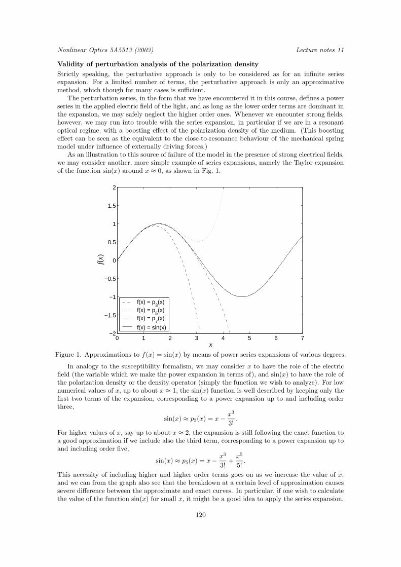
Nonlinear Optics 5A5513 (2003) Lecture notes 11
Validity of perturbation analysis of the polarization density
Strictly speaking, the perturbative approach is only to be considered as for an infinite seriesexpansion. For a limited number of terms, the perturbative approach is only an approximativemethod, which though for many cases is sufficient.
The perturbation series, in the form that we have encountered it in this course, defines a powerseries in the applied electric field of the light, and as long as the lower order terms are dominant inthe expansion, we may safely neglect the higher order ones. Whenever we encounter strong fields,however, we may run into trouble with the series expansion, in particular if we are in a resonantoptical regime, with a boosting effect of the polarization density of the medium. (This boostingeffect can be seen as the equivalent to the close-to-resonance behaviour of the mechanical springmodel under influence of externally driving forces.)
As an illustration to this source of failure of the model in the presence of strong electrical fields,we may consider another, more simple example of series expansions, namely the Taylor expansionof the function sin(x) around x ≈ 0, as shown in Fig. 1.
0 1 2 3 4 5 6 7−2
−1.5
−1
−0.5
0
0.5
1
1.5
2
x
f(x)
f(x) = p3(x)
f(x) = p5(x)
f(x) = p7(x)
f(x) = sin(x)
Figure 1. Approximations to f(x) = sin(x) by means of power series expansions of various degrees.
In analogy to the susceptibility formalism, we may consider x to have the role of the electricfield (the variable which we make the power expansion in terms of), and sin(x) to have the role ofthe polarization density or the density operator (simply the function we wish to analyze). For lownumerical values of x, up to about x ≈ 1, the sin(x) function is well described by keeping only thefirst two terms of the expansion, corresponding to a power expansion up to and including orderthree,
sin(x) ≈ p3(x) = x− x3
3!.
For higher values of x, say up to about x ≈ 2, the expansion is still following the exact function toa good approximation if we include also the third term, corresponding to a power expansion up toand including order five,
sin(x) ≈ p5(x) = x− x3
3!+x5
5!.
This necessity of including higher and higher order terms goes on as we increase the value of x,and we can from the graph also see that the breakdown at a certain level of approximation causessevere difference between the approximate and exact curves. In particular, if one wish to calculatethe value of the function sin(x) for small x, it might be a good idea to apply the series expansion.
120
Lecture notes 11 Nonlinear Optics 5A5513 (2003)
For greater values of x, say x ≈ 10, the series expansion approach is, however, a bad idea, and anefficient evaluation of sin(x) requires another approach.
As a matter of fact, the same arguments hold for the more complex case of the series expansionof the density operator1, for which we for high intensities (high electrical field strengths) mustinclude higher order terms as well.
However, we have seen that even in the non-resonant case, we may encounter great algebraiccomplexity even in low order nonlinear terms, and since the problem of formulating a properpolarization density is expanding more or less exponentially with the order of the nonlinearity, theusefulness of the susceptibility formalism eventually breaks down. The solution to this problem isto identify the relevant transitions of the ensemble, and to solve the equation of motion (2) exactlyinstead (or at least within other levels of approximation which do not rely on the perturbativefoundation of the susceptibility formalism).
The two-level system
In many cases, the interaction between light and matter can be reduced to that of a two-levelsystem, consisting of only two energy eigenstates |a〉 and |b〉. The equation of motion of thedensity operator is generally given by Eq. (2) as
i~dρ
dt= [H, ρ],
with
H = H0 + HI(t) + HR.
For the two-level system, the equation of motion can be expressed in terms of the matrix elementsof the density operator as
i~dρaadt
= [H0, ρ]aa + [HI(t), ρ]aa + [HR, ρ]aa, (3a)
i~dρabdt
= [H0, ρ]ab + [HI(t), ρ]ab + [HR, ρ]ab, (3b)
i~dρbbdt
= [H0, ρ]bb + [HI(t), ρ]bb + [HR, ρ]bb, (3c)
where the fourth equation for ρba was omitted, since the solution for this element immediatelyfollows from
ρba = ρ∗ab.
Terms involving the thermal equilibrium Hamiltonian
The system of Eqs. (3) is the starting point for derivation of the so-called Bloch equations. Startingwith the thermal-equilibrium part of the commutators in the right-hand sides of Eqs. (3), we havefor the diagonal elements
[H0, ρ]aa = 〈a|H0ρ|a〉 − 〈a|ρH0|a〉=
∑
k
〈a|H0|k〉︸ ︷︷ ︸=Eaδak
〈k|ρ|a〉 −∑
j
〈a|ρ|j〉 〈j|H0|a〉︸ ︷︷ ︸=Ejδja
= Eaρaa − ρaaEa
= 0
= [H0, ρ]bb,
1 We may recall that the series expansion of the density operator is the very origin of the expansionof the polarization density of the medium in terms of the electric field, and hence also the veryfoundation for the whole susceptibility formalism as described in this course.
121

Nonlinear Optics 5A5513 (2003) Lecture notes 11
and for the off-diagonal elements
[H0, ρ]ab = 〈a|H0ρ|b〉 − 〈a|ρH0|b〉=
∑
k
〈a|H0|k〉︸ ︷︷ ︸=Eaδak
〈k|ρ|b〉 −∑
j
〈a|ρ|j〉 〈j|H0|b〉︸ ︷︷ ︸=Ejδjb
= Eaρab − ρabEb
= −(Eb − Ea)ρab
= −~Ωbaρab
Terms involving the interaction Hamiltonian
For the commutators in the right-hand sides of Eqs. (3) involving the interaction Hamiltonian, wesimilarly have for the diagonal elements
[HI(t), ρ]aa = 〈a|(−erαEα(r, t))ρ|a〉 − 〈a|ρ(−erαEα(r, t))|a〉
= −eEα(r, t)
∑
k
〈a|rα|k〉〈k|ρ|a〉 −∑
j
〈a|ρ|j〉〈j|rα|a〉
= −eEα(r, t)
rαaaρaa + rαabρba − ρaar
αaa − ρabr
αba
= −e(rαabρba − rαbaρab)Eα(r, t)
= −[HI(t), ρ]bb,
and for the off-diagonal elements
[HI(t), ρ]ab = 〈a|(−erαEα(r, t))ρ|b〉 − 〈a|ρ(−erαEα(r, t))|b〉
= −eEα(r, t)
∑
k
〈a|rα|k〉〈k|ρ|b〉 −∑
j
〈a|ρ|j〉〈j|rα|b〉
= −eEα(r, t)
rαaaρab + rαabρbb − ρaar
αab − ρabr
αbb
= −erαabEα(r, t)(ρbb − ρaa) − e(rαaa − rαbb)Eα(r, t)ρab
= Optical Stark shift : δEk ≡ −erαkkEα(r, t), k = a, b= −erαabEα(r, t)(ρbb − ρaa) + (δEa − δEb)ρab.
Terms involving relaxation processes
For the commutators describing relaxation processes, the diagonal elements are given as
[HR, ρ]aa = −i~(ρaa − ρ0(a))/Ta,
[HR, ρ]bb = −i~(ρbb − ρ0(b))/Tb,
where Ta and Tb are the decay rates towards the thermal equilibrium at respective level, and whereρ0(a) and ρ0(b) are the thermal equilibrium values of ρaa and ρbb, respectively (i. e. the thermalequilibrium population densities of the respective level). The off-diagonal elements are similarlygiven as
[HR, ρ]ab = −i~ρab/T2,
[HR, ρ]ba = −i~ρba/T2.
A common approximation is to consider the two states |a〉 and |b〉 to be sufficiently similar inorder to approximate their lifetimes as equal, i. e. Ta ≈ Tb ≈ T1, where T1 for historical reasons
122

Lecture notes 11 Nonlinear Optics 5A5513 (2003)
is denoted as the longitudinal relaxation time. For the same historical reason, the relaxation timeT2 is denoted as the transverse relaxation time.2
As the above matrix elements of the commutators involving the various terms of the Hamilto-nian are inserted into the right-hand sides of Eqs. (3), one obtains the following system of equationsfor the matrix elements of the density operator,
i~dρaadt
= −e(rαabρba − rαbaρab)Eα(r, t) − i~(ρaa − ρ0(a))/Ta, (4a)
i~dρabdt
= −~Ωbaρab − erαabEα(r, t)(ρbb − ρaa) + (δEa − δEb)ρab − i~ρab/T2, (4b)
i~dρbbdt
= e(rαabρba − rαbaρab)Eα(r, t) − i~(ρbb − ρ0(b))/Tb. (4c)
(The system of equations (4) corresponds to Butcher and Cotter’s Eqs. (6.35).) So far, the appliedelectric field of the light is allowed to be of arbitrary form. However, in order to simplify thefollowing analysis, we will assume the light to be linearly polarized and quasimonochromatic, ofthe form
Eα(r, t) = Re[Eαω(t) exp(−iωt)].
We will in addition assume the slowly varying temporal envelope Eαω (t) to be real-valued, and wewill also neglect the optical Stark shifts δEa and δEb. In the absence of strong static magneticfields, we may also assume the matrix elements erαab to be real-valued. When these assumptionsand approximations are applied to the equations of motion (4), one obtains
dρaadt
= i(ρba − ρab)β(t) cos(ωt) − (ρaa − ρ0(a))/Ta, (5a)
dρabdt
= iΩbaρab + iβ(t) cos(ωt)(ρbb − ρaa) − ρab/T2, (5b)
dρbbdt
= −i(ρba − ρab)β(t) cos(ωt) − (ρbb − ρ0(b))/Tb, (5c)
where the Rabi frequency β(t), defined in terms of the spatial envelope of the electrical field andthe transition dipole moment as
β(t) = erαabEαω(t)/~ = erab · Eω(t)/~,
was introduced.
The rotating-wave approximation
In the middle equation of the system (5), we have a time-derivative of ρab in the left-hand side,while we in the right-hand side have a term iΩbaρab. Seen as the homogeneous part of a lineardifferential equation, this suggests that we may further simplify the equations of motion by takinga new variable ρΩ
ab according to the variable substitution
ρab = ρΩab exp[i(Ωba − ∆)t], (6)
where ∆ ≡ Ωba − ω is the detuning of the angular frequency of the light from the transitionfrequency Ωba ≡ (Eb − Ea)/~.
2 For a deeper discusssion and explanation of the various mechanisms involved in relaxation,see for example Charles P. Slichter, Principles of Magnetic Resonance (Springer-Verlag, Berlin,1978), available at KTHB. This reference is not mentioned in Butcher and Cotters book, but it isa very good text on relaxation phenomena and how to incorporate them into a density-functionaldescription of interaction between light and matter.
123

Nonlinear Optics 5A5513 (2003) Lecture notes 11
By inserting Eq. (6) into Eqs. (5), keeping in mind that ρba = ρ∗ab, one obtains the system
dρaadt
= i(ρΩba exp[−i(Ωba − ∆)t] − ρΩ
ab exp[i(Ωba − ∆)t])β(t) cos(ωt) − (ρaa − ρ0(a))/Ta, (6a)
dρΩab
dt= i∆ρΩ
ab + iβ(t) cos(ωt) exp[−i(Ωba − ∆)t](ρbb − ρaa) − ρΩab/T2, (6b)
dρbbdt
= −i(ρΩba exp[−i(Ωba − ∆)t] − ρΩ
ab exp[i(Ωba − ∆)t])β(t) cos(ωt) − (ρbb − ρ0(b))/Tb, (6c)
The idea with the rotating-wave approximation is now to separate out rapidly oscillating terms ofangular frequencies ω+ Ωba and −(ω+ Ωba), and neglect these terms, compared with more slowlyvarying terms. The motivation for this approximation is that whenever high-frequency componentsappear in the equations of motions, the high-frequency terms will when integrated contain largedenominators, and will hence be minor in comparison with terms with a slow variation. In somesense we can also see this as a temporal averaging procedure, where rapidly oscillating termsaverage to zero rapidly compared to slowly varying (or constant) components.
For example, in Eq. (6b), the product of the cos(ωt) and the exponential function is approxi-mated as
cos(ωt) exp[−i(Ωba − ∆)t] =1
2[exp(iωt) + exp(−iωt)] exp[−i (Ωba − ∆)︸ ︷︷ ︸
=ω
t]
=1
2[1 + exp(−i2ωt)] → 1
2,
while in Eqs. (6a) and (6c), the same argument gives
exp[i(Ωba − ∆)t] cos(ωt) =1
2[exp(iωt) + exp(−iωt)] exp[−i (Ωba − ∆)︸ ︷︷ ︸
=ω
t]
=1
2[exp(i2ωt) + 1] → 1
2.
By applying this rotating-wave approximation, the equations of motion (6) hence take the form
dρaadt
=i
2(ρΩba − ρΩ
ab)β(t) − (ρaa − ρ0(a))/Ta, (7a)
dρΩab
dt= i∆ρΩ
ab +i
2β(t)(ρbb − ρaa) − ρΩ
ab/T2, (7b)
dρbbdt
= − i
2(ρΩba − ρΩ
ab)β(t) − (ρbb − ρ0(b))/Tb. (7c)
In this final form, before entering the Bloch vector description of the interaction, these equationscorrespond to Butcher and Cotter’s Eqs. (6.41).
The Bloch equations
Assuming the two states |a〉 and |b〉 to be sufficiently similar in order to approximate Ta ≈ Tb ≈ T1,where T1 is the longitudinal relaxation time, and by taking new variables (u, v, w) according to
u = ρΩba + ρΩ
ab,
v = i(ρΩba − ρΩ
ab),
w = ρbb − ρaa,
the equations of motion (7) are cast in the Bloch equations
du
dt= −∆v − u/T2, (8a)
dv
dt= ∆u+ β(t)w − v/T2, (8b)
dw
dt= −β(t)v − (w − w0)/T1. (8c)
124
Lecture notes 11 Nonlinear Optics 5A5513 (2003)
In these equations, the introduced variable w describes the population inversion of the two-levelsystem, while u and v are related to the dispersive and absorptive components of the polarizationdensity of the medium. In the Bloch equations above, w0 = ρ0(b)−ρ0(a) is the thermal equilibriuminversion of the system with no optical field applied.
The resulting electric polarization density of the medium
The so far developed theory of the density matrix under resonant interaction can now be appliedto the calculation of the electric polarization density of the medium, consisting of N identicalmolecules per unit volume, as
Pµ(r, t) = N〈erµ〉= N Tr[ρerµ]
= N∑
k=a,b
〈k|ρerµ|k〉
= N∑
k=a,b
∑
j=a,b
〈k|ρ|j〉〈j|erµ|k〉
= N∑
k=a,b
〈k|ρ|a〉〈a|erµ|k〉 + 〈k|ρ|b〉〈b|erµ|k〉
= N 〈a|ρ|a〉〈a|erµ|a〉 + 〈b|ρ|a〉〈a|erµ|b〉 + 〈a|ρ|b〉〈b|erµ|a〉 + 〈b|ρ|b〉〈b|erµ|b〉= N(ρbaer
µab + ρaber
µba)
= Make use of ρab = (u+ iv) exp(iωt) = ρ∗ba= N [(u− iv) exp(−iωt)erµab + (u+ iv) exp(iωt)erµba].
The temporal envelope P µω of the polarization density, throughout this course as well as in Butcherand Cotter’s book, is taken as
Pµ(r, t) = Re[Pµω exp(−iωt)],
and by identifying this expression with the right-hand side of the result above, we hence finallyhave obtained the polarization density in terms of the Bloch parameters (u, v, w) as
Pµω (r, t) = Nerµab(u− iv).
This expression for the temporal envelope of the polarization density is exactly in the same modeof description as the one as previously used in the susceptibility theory, as in the wave equationsdeveloped in lecture eight. The only difference is that now we instead consider the polarizationdensity as given by a non-perturbative analysis. Taken together with the Maxwell’s equations (orthe proper wave equation for the envelopes of the fields), the Bloch equations are known as theMaxwell–Bloch equations.
125

Nonlinear Optics 5A5513 (2003) Lecture notes 11
126

Lecture Notes on Nonlinear Optics Nonlinear Optics 5A5513 (2003)
Lecture XII
127

Nonlinear Optics 5A5513 (2003) Lecture Notes on Nonlinear Optics
Lecture Notes on Nonlinear OpticsNonlinear Optics (5A5513, 5p for advanced undergraduate and doctoral students)Course given at the Royal Institute of Technology,Department of Laser Physics and Quantum OpticsSE–106 91, Stockholm, SwedenJanuary 8 – March 24, 2003
The texts and figures in this lecture series was typeset by the author in 10/12/16 pt ComputerModern typeface using plain TEX and METAPOST.
This document is electronically available at the homepage of the Library of the Royal Institute ofTechnology, at http://www.lib.kth.se.
Copyright c© Fredrik Jonsson 2003
All rights reserved. No part of this publication may be reproduced, stored in a retrieval system,or transmitted, in any form, or by any means, electronic, mechanical, photo-copying, recording, orotherwise, without the prior consent of the author.
ISBN 91-7283-517-6TRITA-FYS 2003:26ISSN 0280-316XISRN KTH/FYS/- - 03:26 - - SEPrinted on July 7, 2003
TEX is a trademark of the American Mathematical Society
128

Nonlinear Optics 5A5513 (2003)Lecture notes
Lecture 12
In this final lecture, we will study the behaviour of the Bloch equations in different regimes ofresonance and relaxation. The Bloch equations are formulated as a vector model, and numericalsolutions to the equations are discussed.
For steady-state interaction, the polarization density of the medium, as obtained from theBloch equations, is expressed in a closed form. The closed solution is then expanded in a powerseries, which when compared with the series obtained from the susceptibility formalism finally tietogether the Bloch theory with the susceptibilities.
The outline for this lecture is:• Recapitulation of the Bloch equations• The vector model of the Bloch equations• Special cases and examples• Steady-state regime• The intensity dependent refractive index at steady-state• Comparison with the susceptibility model
Recapitulation of the Bloch equations for two-level systems
Assuming two states |a〉 and |b〉 to be sufficiently similar in order for their respective lifetimes Ta ≈Tb ≈ T1 to hold, where T1 is the longitudinal relaxation time, the Bloch equations for the two-levelare given as
du
dt= −∆v − u/T2, (1a)
dv
dt= ∆u+ β(t)w − v/T2, (1b)
dw
dt= −β(t)v − (w − w0)/T1, (1c)
where β ≡ erαabEαω(t)/~ is the Rabi frequency, being a quantity linear in the applied electric field
of the light, ∆ ≡ Ωba − ω is the detuning of the angular frequency of the light from the transitionfrequency Ωba ≡ (Eb − Ea)/~, and where the variables (u, v, w) are related to the matrix elementsρmn of the density operator as
u = ρΩba + ρΩ
ab,
v = i(ρΩba − ρΩ
ab),
w = ρbb − ρaa.
In these equations, ρΩab is the temporal envelope of the off-diagonal elements, given by
ρab ≡ ρΩab exp[i(Ωba − ∆)t].
In the Bloch equations (1), the variable w describes the population inversion of the two-levelsystem, while u and v are related to the dispersive and absorptive components of the polarizationdensity of the medium. In the Bloch equations, w0 ≡ ρ0(b) − ρ0(a) is the thermal equilibriuminversion of the system with no optical field applied.
129
Nonlinear Optics 5A5513 (2003) Lecture notes 12
The resulting electric polarization density of the medium
The so far developed theory of the density matrix under resonant interaction can now be appliedto the calculation of the electric polarization density of the medium, consisting of N identicalmolecules per unit volume, as
Pµ(r, t) = N〈erµ〉= N Tr[ρerµ]
= N∑
k=a,b
〈k|ρerµ|k〉
= N∑
k=a,b
∑
j=a,b
〈k|ρ|j〉〈j|erµ|k〉
= N∑
k=a,b
〈k|ρ|a〉〈a|erµ|k〉 + 〈k|ρ|b〉〈b|erµ|k〉
= N 〈a|ρ|a〉〈a|erµ|a〉 + 〈b|ρ|a〉〈a|erµ|b〉 + 〈a|ρ|b〉〈b|erµ|a〉 + 〈b|ρ|b〉〈b|erµ|b〉= N(ρbaer
µab + ρaber
µba)
= Make use of ρab = (u+ iv) exp(iωt) = ρ∗ba= N [(u− iv) exp(−iωt)erµab + (u+ iv) exp(iωt)erµba].
The temporal envelope P µω of the polarization density is throughout this course as well as in Butcherand Cotter’s book taken as
Pµ(r, t) = Re[Pµω exp(−iωt)],
and by identifying this expression with the right-hand side of the result above, we hence finallyhave obtained the polarization density in terms of the Bloch parameters (u, v, w) as
Pµω (r, t) = Nerµab(u− iv). (2)
This expression for the temporal envelope of the polarization density is exactly in the same modeof description as the one as previously used in the susceptibility theory, as in the wave equationsdeveloped in lecture eight. The only difference is that now we instead consider the polarizationdensity as given by a non-perturbative analysis. Taken together with the Maxwell’s equations (orthe propern wave equation for the envelopes of the fields), the Bloch equations are known as theMaxwell–Bloch equations.
From Eq. (2), it should now be clear that the Bloch variable u essentially gives the in-phasepart of the polarization density (at least in this case, where we may consider the transition dipolemoments to be real-valued), corresponding to the dispersive components of the interaction betweenlight and matter, while the Bloch variable v on the other hand gives terms which are shifted ninetydegrees out of phase with the optical field, hence corresponding to absorptive terms.
130
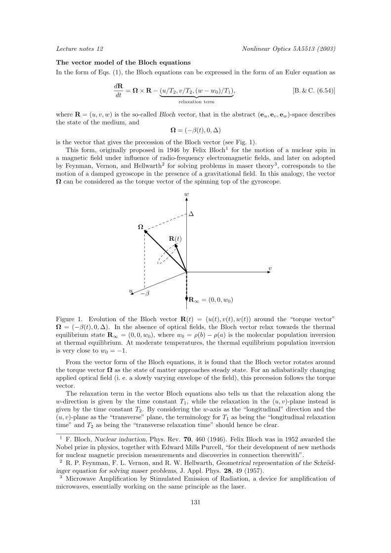
Lecture notes 12 Nonlinear Optics 5A5513 (2003)
The vector model of the Bloch equations
In the form of Eqs. (1), the Bloch equations can be expressed in the form of an Euler equation as
dR
dt= Ω × R − (u/T2, v/T2, (w − w0)/T1)︸ ︷︷ ︸
relaxation term
, [B.& C. (6.54)]
where R = (u, v, w) is the so-called Bloch vector, that in the abstract (eu, ev, ew)-space describesthe state of the medium, and
Ω = (−β(t), 0,∆)
is the vector that gives the precession of the Bloch vector (see Fig. 1).This form, originally proposed in 1946 by Felix Bloch1 for the motion of a nuclear spin in
a magnetic field under influence of radio-frequency electromagnetic fields, and later on adoptedby Feynman, Vernon, and Hellwarth2 for solving problems in maser theory3, corresponds to themotion of a damped gyroscope in the presence of a gravitational field. In this analogy, the vectorΩ can be considered as the torque vector of the spinning top of the gyroscope.
u
v
w
Ω
R(t)
R∞ = (0, 0, w0)−β
∆
Figure 1. Evolution of the Bloch vector R(t) = (u(t), v(t), w(t)) around the “torque vector”Ω = (−β(t), 0,∆). In the absence of optical fields, the Bloch vector relax towards the thermalequilibrium state R∞ = (0, 0, w0), where w0 = ρ(b) − ρ(a) is the molecular population inversionat thermal equilibrium. At moderate temperatures, the thermal equilibrium population inversionis very close to w0 = −1.
From the vector form of the Bloch equations, it is found that the Bloch vector rotates aroundthe torque vector Ω as the state of matter approaches steady state. For an adiabatically changingapplied optical field (i. e. a slowly varying envelope of the field), this precession follows the torquevector.
The relaxation term in the vector Bloch equations also tells us that the relaxation along thew-direction is given by the time constant T1, while the relaxation in the (u, v)-plane instead isgiven by the time constant T2. By considering the w-axis as the “longitudinal” direction and the(u, v)-plane as the “transverse” plane, the terminology for T1 as being the “longitudinal relaxationtime” and T2 as being the “transverse relaxation time” should hence be clear.
1 F. Bloch, Nuclear induction, Phys. Rev. 70, 460 (1946). Felix Bloch was in 1952 awarded theNobel prize in physics, together with Edward Mills Purcell, “for their development of new methodsfor nuclear magnetic precision measurements and discoveries in connection therewith”.
2 R. P. Feynman, F. L. Vernon, and R. W. Hellwarth, Geometrical representation of the Schrod-inger equation for solving maser problems, J. Appl. Phys. 28, 49 (1957).
3 Microwave Amplification by Stimulated Emission of Radiation, a device for amplification ofmicrowaves, essentially working on the same principle as the laser.
131
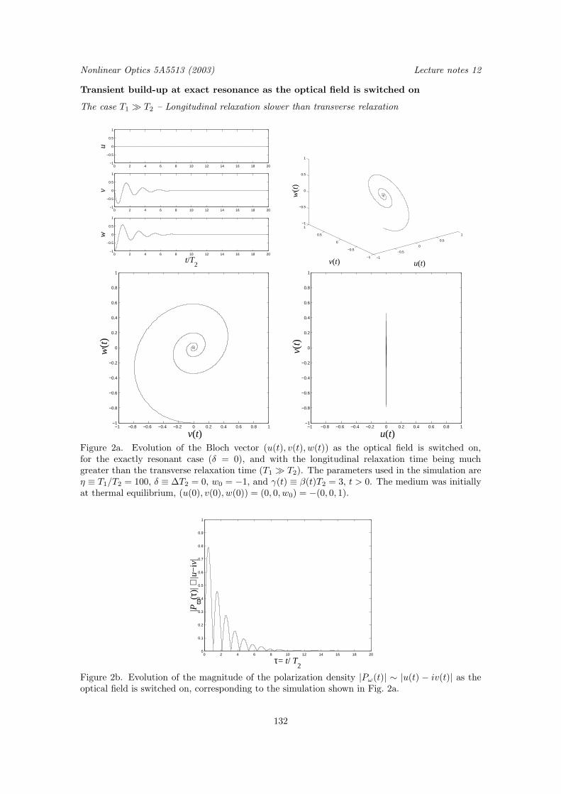
Nonlinear Optics 5A5513 (2003) Lecture notes 12
Transient build-up at exact resonance as the optical field is switched on
The case T1 T2 – Longitudinal relaxation slower than transverse relaxation
0 2 4 6 8 10 12 14 16 18 20−1
−0.5
0
0.5
1
u
0 2 4 6 8 10 12 14 16 18 20−1
−0.5
0
0.5
1
v
0 2 4 6 8 10 12 14 16 18 20−1
−0.5
0
0.5
1
t/T2
w
−1
−0.5
0
0.5
1
−1
−0.5
0
0.5
1−1
−0.5
0
0.5
1
u(t) v(t)
w(t
)
−1 −0.8 −0.6 −0.4 −0.2 0 0.2 0.4 0.6 0.8 1−1
−0.8
−0.6
−0.4
−0.2
0
0.2
0.4
0.6
0.8
1
v(t)
w(t
)
−1 −0.8 −0.6 −0.4 −0.2 0 0.2 0.4 0.6 0.8 1−1
−0.8
−0.6
−0.4
−0.2
0
0.2
0.4
0.6
0.8
1
u(t)
v(t
)
Figure 2a. Evolution of the Bloch vector (u(t), v(t), w(t)) as the optical field is switched on,for the exactly resonant case (δ = 0), and with the longitudinal relaxation time being muchgreater than the transverse relaxation time (T1 T2). The parameters used in the simulation areη ≡ T1/T2 = 100, δ ≡ ∆T2 = 0, w0 = −1, and γ(t) ≡ β(t)T2 = 3, t > 0. The medium was initiallyat thermal equilibrium, (u(0), v(0), w(0)) = (0, 0, w0) = −(0, 0, 1).
0 2 4 6 8 10 12 14 16 18 200
0.1
0.2
0.3
0.4
0.5
0.6
0.7
0.8
0.9
1
τ= t/ T2
|Pω
(τ)|
∼ |u
−iv
|
Figure 2b. Evolution of the magnitude of the polarization density |Pω(t)| ∼ |u(t) − iv(t)| as theoptical field is switched on, corresponding to the simulation shown in Fig. 2a.
132
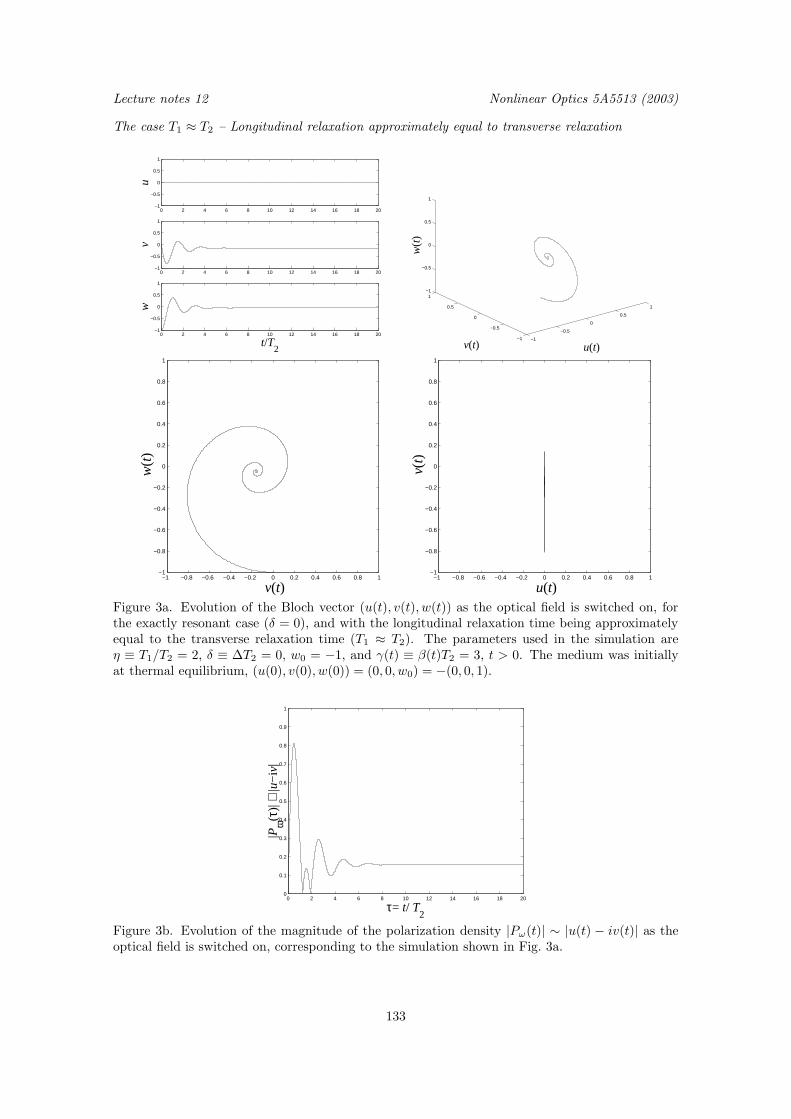
Lecture notes 12 Nonlinear Optics 5A5513 (2003)
The case T1 ≈ T2 – Longitudinal relaxation approximately equal to transverse relaxation
0 2 4 6 8 10 12 14 16 18 20−1
−0.5
0
0.5
1
u
0 2 4 6 8 10 12 14 16 18 20−1
−0.5
0
0.5
1
v
0 2 4 6 8 10 12 14 16 18 20−1
−0.5
0
0.5
1
t/T2
w
−1
−0.5
0
0.5
1
−1
−0.5
0
0.5
1−1
−0.5
0
0.5
1
u(t) v(t)
w(t
)
−1 −0.8 −0.6 −0.4 −0.2 0 0.2 0.4 0.6 0.8 1−1
−0.8
−0.6
−0.4
−0.2
0
0.2
0.4
0.6
0.8
1
v(t)
w(t
)
−1 −0.8 −0.6 −0.4 −0.2 0 0.2 0.4 0.6 0.8 1−1
−0.8
−0.6
−0.4
−0.2
0
0.2
0.4
0.6
0.8
1
u(t)
v(t
)
Figure 3a. Evolution of the Bloch vector (u(t), v(t), w(t)) as the optical field is switched on, forthe exactly resonant case (δ = 0), and with the longitudinal relaxation time being approximatelyequal to the transverse relaxation time (T1 ≈ T2). The parameters used in the simulation areη ≡ T1/T2 = 2, δ ≡ ∆T2 = 0, w0 = −1, and γ(t) ≡ β(t)T2 = 3, t > 0. The medium was initiallyat thermal equilibrium, (u(0), v(0), w(0)) = (0, 0, w0) = −(0, 0, 1).
0 2 4 6 8 10 12 14 16 18 200
0.1
0.2
0.3
0.4
0.5
0.6
0.7
0.8
0.9
1
τ= t/ T2
|Pω
(τ)|
∼ |u
−iv
|
Figure 3b. Evolution of the magnitude of the polarization density |Pω(t)| ∼ |u(t) − iv(t)| as theoptical field is switched on, corresponding to the simulation shown in Fig. 3a.
133

Nonlinear Optics 5A5513 (2003) Lecture notes 12
Transient build-up at off-resonance as the optical field is switched on
The case T1 ≈ T2 – Longitudinal relaxation approximately equal to transverse relaxation
0 2 4 6 8 10 12 14 16 18 20−1
−0.5
0
0.5
1
u
0 2 4 6 8 10 12 14 16 18 20−1
−0.5
0
0.5
1
v
0 2 4 6 8 10 12 14 16 18 20−1
−0.5
0
0.5
1
t/T2
w
−1
−0.5
0
0.5
1
−1
−0.5
0
0.5
1−1
−0.5
0
0.5
1
u(t) v(t)
w(t
)
−1 −0.8 −0.6 −0.4 −0.2 0 0.2 0.4 0.6 0.8 1−1
−0.8
−0.6
−0.4
−0.2
0
0.2
0.4
0.6
0.8
1
v(t)
w(t
)
−1 −0.8 −0.6 −0.4 −0.2 0 0.2 0.4 0.6 0.8 1−1
−0.8
−0.6
−0.4
−0.2
0
0.2
0.4
0.6
0.8
1
u(t)
v(t
)
Figure 4a. Evolution of the Bloch vector (u(t), v(t), w(t)) as the optical field is switched on,for the off-resonant case (δ 6= 0), and with the longitudinal relaxation time being approximatelyequal to the transverse relaxation time (T1 ≈ T2). The parameters used in the simulation areη ≡ T1/T2 = 2, δ ≡ ∆T2 = 4, w0 = −1, and γ(t) ≡ β(t)T2 = 3, t > 0. The medium was initiallyat thermal equilibrium, (u(0), v(0), w(0)) = (0, 0, w0) = −(0, 0, 1).
0 2 4 6 8 10 12 14 16 18 200
0.1
0.2
0.3
0.4
0.5
0.6
0.7
0.8
0.9
1
τ= t/ T2
|Pω
(τ)|
∼ |u
−iv
|
Figure 4b. Evolution of the magnitude of the polarization density |Pω(t)| ∼ |u(t) − iv(t)| as theoptical field is switched on, corresponding to the simulation shown in Fig. 4a.
134
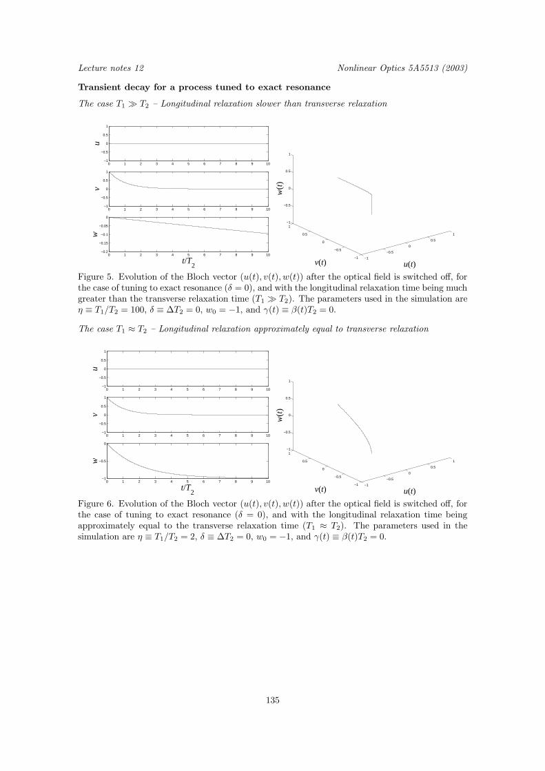
Lecture notes 12 Nonlinear Optics 5A5513 (2003)
Transient decay for a process tuned to exact resonance
The case T1 T2 – Longitudinal relaxation slower than transverse relaxation
0 1 2 3 4 5 6 7 8 9 10−1
−0.5
0
0.5
1
u
0 1 2 3 4 5 6 7 8 9 10−1
−0.5
0
0.5
1
v
0 1 2 3 4 5 6 7 8 9 10−0.2
−0.15
−0.1
−0.05
0
t/T2
w
−1
−0.5
0
0.5
1
−1
−0.5
0
0.5
1−1
−0.5
0
0.5
1
u(t) v(t)
w(t
)Figure 5. Evolution of the Bloch vector (u(t), v(t), w(t)) after the optical field is switched off, forthe case of tuning to exact resonance (δ = 0), and with the longitudinal relaxation time being muchgreater than the transverse relaxation time (T1 T2). The parameters used in the simulation areη ≡ T1/T2 = 100, δ ≡ ∆T2 = 0, w0 = −1, and γ(t) ≡ β(t)T2 = 0.
The case T1 ≈ T2 – Longitudinal relaxation approximately equal to transverse relaxation
0 1 2 3 4 5 6 7 8 9 10−1
−0.5
0
0.5
1
u
0 1 2 3 4 5 6 7 8 9 10−1
−0.5
0
0.5
1
v
0 1 2 3 4 5 6 7 8 9 10−1
−0.5
0
t/T2
w
−1
−0.5
0
0.5
1
−1
−0.5
0
0.5
1−1
−0.5
0
0.5
1
u(t) v(t)
w(t
)
Figure 6. Evolution of the Bloch vector (u(t), v(t), w(t)) after the optical field is switched off, forthe case of tuning to exact resonance (δ = 0), and with the longitudinal relaxation time beingapproximately equal to the transverse relaxation time (T1 ≈ T2). The parameters used in thesimulation are η ≡ T1/T2 = 2, δ ≡ ∆T2 = 0, w0 = −1, and γ(t) ≡ β(t)T2 = 0.
135
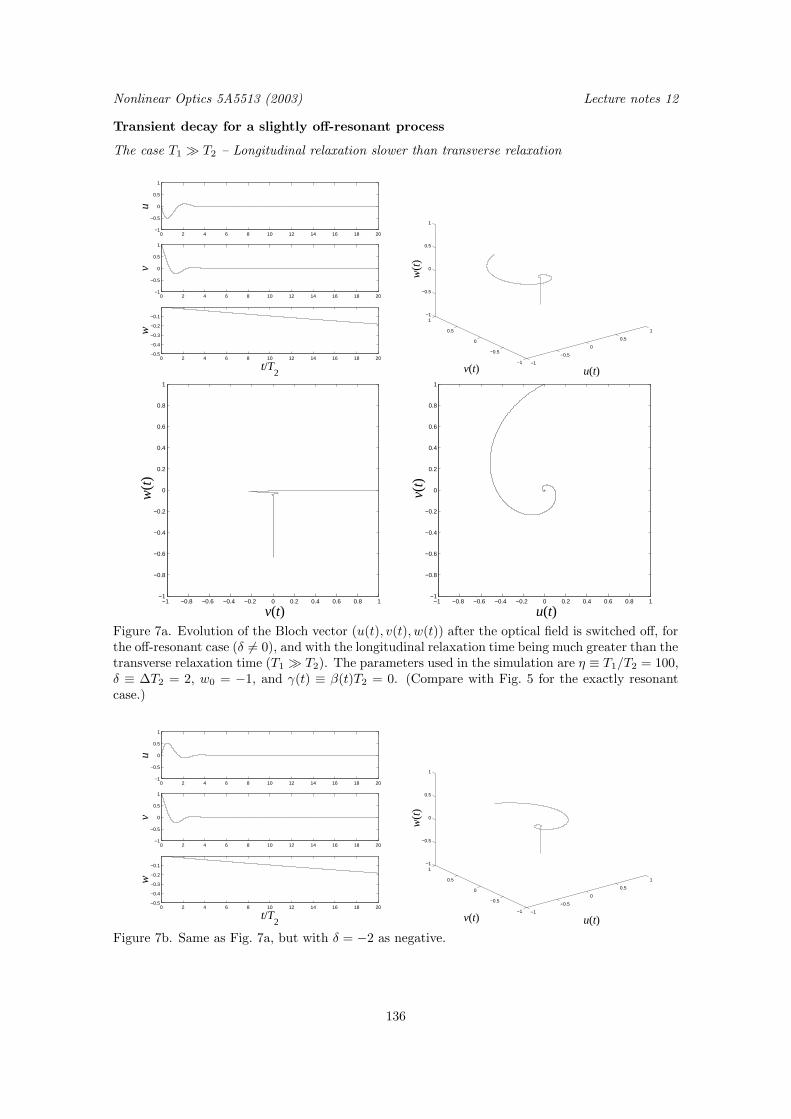
Nonlinear Optics 5A5513 (2003) Lecture notes 12
Transient decay for a slightly off-resonant process
The case T1 T2 – Longitudinal relaxation slower than transverse relaxation
0 2 4 6 8 10 12 14 16 18 20−1
−0.5
0
0.5
1
u
0 2 4 6 8 10 12 14 16 18 20−1
−0.5
0
0.5
1
v
0 2 4 6 8 10 12 14 16 18 20−0.5
−0.4
−0.3
−0.2
−0.1
t/T2
w
−1
−0.5
0
0.5
1
−1
−0.5
0
0.5
1−1
−0.5
0
0.5
1
u(t) v(t)
w(t
)
−1 −0.8 −0.6 −0.4 −0.2 0 0.2 0.4 0.6 0.8 1−1
−0.8
−0.6
−0.4
−0.2
0
0.2
0.4
0.6
0.8
1
v(t)
w(t
)
−1 −0.8 −0.6 −0.4 −0.2 0 0.2 0.4 0.6 0.8 1−1
−0.8
−0.6
−0.4
−0.2
0
0.2
0.4
0.6
0.8
1
u(t)
v(t
)
Figure 7a. Evolution of the Bloch vector (u(t), v(t), w(t)) after the optical field is switched off, forthe off-resonant case (δ 6= 0), and with the longitudinal relaxation time being much greater than thetransverse relaxation time (T1 T2). The parameters used in the simulation are η ≡ T1/T2 = 100,δ ≡ ∆T2 = 2, w0 = −1, and γ(t) ≡ β(t)T2 = 0. (Compare with Fig. 5 for the exactly resonantcase.)
0 2 4 6 8 10 12 14 16 18 20−1
−0.5
0
0.5
1
u
0 2 4 6 8 10 12 14 16 18 20−1
−0.5
0
0.5
1
v
0 2 4 6 8 10 12 14 16 18 20−0.5
−0.4
−0.3
−0.2
−0.1
t/T2
w
−1
−0.5
0
0.5
1
−1
−0.5
0
0.5
1−1
−0.5
0
0.5
1
u(t) v(t)
w(t
)
Figure 7b. Same as Fig. 7a, but with δ = −2 as negative.
136

Lecture notes 12 Nonlinear Optics 5A5513 (2003)
The case T1 ≈ T2 – Longitudinal relaxation approximately equal to transverse relaxation
0 2 4 6 8 10 12 14 16 18 20
−0.4
−0.2
0
0.2
u
0 2 4 6 8 10 12 14 16 18 20−0.5
0
0.5
1
v
0 2 4 6 8 10 12 14 16 18 20−1
−0.5
0
t/T2
w
−1
−0.5
0
0.5
1
−1
−0.5
0
0.5
1−1
−0.5
0
0.5
1
u(t) v(t)
w(t
)
−1 −0.8 −0.6 −0.4 −0.2 0 0.2 0.4 0.6 0.8 1−1
−0.8
−0.6
−0.4
−0.2
0
0.2
0.4
0.6
0.8
1
v(t)
w(t
)
−1 −0.8 −0.6 −0.4 −0.2 0 0.2 0.4 0.6 0.8 1−1
−0.8
−0.6
−0.4
−0.2
0
0.2
0.4
0.6
0.8
1
u(t)
v(t
)
Figure 8a. Evolution of the Bloch vector (u(t), v(t), w(t)) after the optical field is switched off,for the off-resonant case (δ 6= 0), and with the longitudinal relaxation time being approximatelyequal to the transverse relaxation time (T1 ≈ T2). The parameters used in the simulation areη ≡ T1/T2 = 2, δ ≡ ∆T2 = 2, w0 = −1, and γ(t) ≡ β(t)T2 = 0. (Compare with Fig. 6 for theexactly resonant case.)
0 2 4 6 8 10 12 14 16 18 200
0.1
0.2
0.3
0.4
0.5
0.6
0.7
0.8
0.9
1
τ= t/ T2
|Pω
(τ)|
∼ |u
−iv
|
Figure 8b. Evolution of the magnitude of the polarization density |Pω(t)| ∼ |u(t) − iv(t)| as theoptical field is switched on, corresponding to the simulation shown in Fig. 8a.
137

Nonlinear Optics 5A5513 (2003) Lecture notes 12
Transient decay for a far off-resonant process
The case T1 T2 – Longitudinal relaxation slower than transverse relaxation
0 2 4 6 8 10 12 14 16 18 20−1
−0.5
0
0.5
1
u
0 2 4 6 8 10 12 14 16 18 20−1
−0.5
0
0.5
1
v
0 2 4 6 8 10 12 14 16 18 20
−0.5
−0.4
−0.3
−0.2
−0.1
t/T2
w
−1
−0.5
0
0.5
1
−1
−0.5
0
0.5
1−1
−0.5
0
0.5
1
u(t) v(t)
w(t
)
−1 −0.8 −0.6 −0.4 −0.2 0 0.2 0.4 0.6 0.8 1−1
−0.8
−0.6
−0.4
−0.2
0
0.2
0.4
0.6
0.8
1
v(t)
w(t
)
−1 −0.8 −0.6 −0.4 −0.2 0 0.2 0.4 0.6 0.8 1−1
−0.8
−0.6
−0.4
−0.2
0
0.2
0.4
0.6
0.8
1
u(t)
v(t
)
Figure 9a. Evolution of the Bloch vector (u(t), v(t), w(t)) after the optical field is switched off, forthe far off-resonant case (δ 6= 0), and with the longitudinal relaxation time being much greaterthan the transverse relaxation time (T1 T2). The parameters used in the simulation are η ≡T1/T2 = 100, δ ≡ ∆T2 = 20, w0 = −1, and γ(t) ≡ β(t)T2 = 0. (Compare with Fig. 5 for theexactly resonant case, and with Fig. 7a for the slightly off-resonant case.)
0 2 4 6 8 10 12 14 16 18 200
0.1
0.2
0.3
0.4
0.5
0.6
0.7
0.8
0.9
1
τ= t/ T2
|Pω
(τ)|
∼ |u
−iv
|
Figure 9b. Evolution of the magnitude of the polarization density |Pω(t)| ∼ |u(t) − iv(t)| as theoptical field is switched on, corresponding to the simulation shown in Fig. 9a.
138
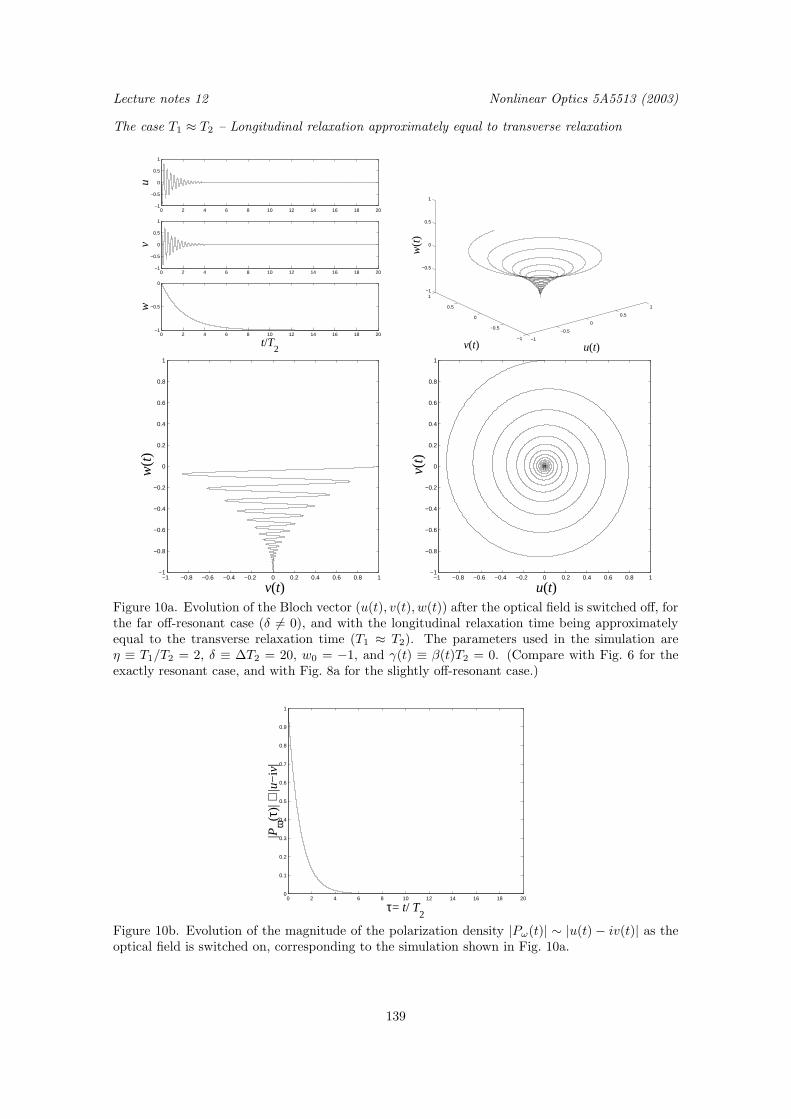
Lecture notes 12 Nonlinear Optics 5A5513 (2003)
The case T1 ≈ T2 – Longitudinal relaxation approximately equal to transverse relaxation
0 2 4 6 8 10 12 14 16 18 20−1
−0.5
0
0.5
1
u
0 2 4 6 8 10 12 14 16 18 20−1
−0.5
0
0.5
1
v
0 2 4 6 8 10 12 14 16 18 20−1
−0.5
0
t/T2
w
−1
−0.5
0
0.5
1
−1
−0.5
0
0.5
1−1
−0.5
0
0.5
1
u(t) v(t)
w(t
)
−1 −0.8 −0.6 −0.4 −0.2 0 0.2 0.4 0.6 0.8 1−1
−0.8
−0.6
−0.4
−0.2
0
0.2
0.4
0.6
0.8
1
v(t)
w(t
)
−1 −0.8 −0.6 −0.4 −0.2 0 0.2 0.4 0.6 0.8 1−1
−0.8
−0.6
−0.4
−0.2
0
0.2
0.4
0.6
0.8
1
u(t)
v(t
)
Figure 10a. Evolution of the Bloch vector (u(t), v(t), w(t)) after the optical field is switched off, forthe far off-resonant case (δ 6= 0), and with the longitudinal relaxation time being approximatelyequal to the transverse relaxation time (T1 ≈ T2). The parameters used in the simulation areη ≡ T1/T2 = 2, δ ≡ ∆T2 = 20, w0 = −1, and γ(t) ≡ β(t)T2 = 0. (Compare with Fig. 6 for theexactly resonant case, and with Fig. 8a for the slightly off-resonant case.)
0 2 4 6 8 10 12 14 16 18 200
0.1
0.2
0.3
0.4
0.5
0.6
0.7
0.8
0.9
1
τ= t/ T2
|Pω
(τ)|
∼ |u
−iv
|
Figure 10b. Evolution of the magnitude of the polarization density |Pω(t)| ∼ |u(t) − iv(t)| as theoptical field is switched on, corresponding to the simulation shown in Fig. 10a.
139
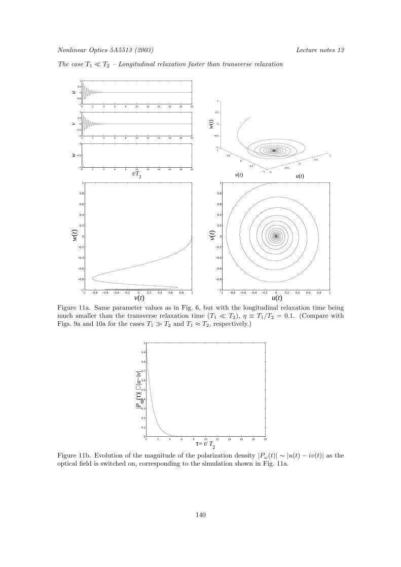
Nonlinear Optics 5A5513 (2003) Lecture notes 12
The case T1 T2 – Longitudinal relaxation faster than transverse relaxation
0 2 4 6 8 10 12 14 16 18 20−1
−0.5
0
0.5
1
u
0 2 4 6 8 10 12 14 16 18 20−1
−0.5
0
0.5
1
v
0 2 4 6 8 10 12 14 16 18 20−1
−0.5
0
t/T2
w
−1
−0.5
0
0.5
1
−1
−0.5
0
0.5
1−1
−0.5
0
0.5
1
u(t) v(t)
w(t
)
−1 −0.8 −0.6 −0.4 −0.2 0 0.2 0.4 0.6 0.8 1−1
−0.8
−0.6
−0.4
−0.2
0
0.2
0.4
0.6
0.8
1
v(t)
w(t
)
−1 −0.8 −0.6 −0.4 −0.2 0 0.2 0.4 0.6 0.8 1−1
−0.8
−0.6
−0.4
−0.2
0
0.2
0.4
0.6
0.8
1
u(t)
v(t
)
Figure 11a. Same parameter values as in Fig. 6, but with the longitudinal relaxation time beingmuch smaller than the transverse relaxation time (T1 T2), η ≡ T1/T2 = 0.1. (Compare withFigs. 9a and 10a for the cases T1 T2 and T1 ≈ T2, respectively.)
0 2 4 6 8 10 12 14 16 18 200
0.1
0.2
0.3
0.4
0.5
0.6
0.7
0.8
0.9
1
τ= t/ T2
|Pω
(τ)|
∼ |u
−iv
|
Figure 11b. Evolution of the magnitude of the polarization density |Pω(t)| ∼ |u(t) − iv(t)| as theoptical field is switched on, corresponding to the simulation shown in Fig. 11a.
140

Lecture notes 12 Nonlinear Optics 5A5513 (2003)
The connection between the Bloch equations and the susceptibility
As an example of the connection between the polarization density obtained from the Bloch equa-tions and the one obtained from the susceptibility formalism, we will now – once again – considerthe intensity-dependent refractive of the medium.
The intensity-dependent refractive index in the susceptibility formalism
Previously in this course, the intensity-dependent refractive index has been obtained from theoptical Kerr-effect in isotropic media, in the form
n = n0 + n2|Eω|2,
where n0 = [1 + χ(1)xx (−ω;ω)]1/2 is the linear refractive index, and
n2 =3
8n0χ(3)xxxx(−ω;ω, ω,−ω)
is the parameter of the intensity dependent contribution. However, since we by now are fully awarethat the polarization density in the description of the susceptibility formalism originally is givenas an infinity series expansion, we may expect that the general form of the intensity dependentrefractive index rather would be as a power series in the intensity,
n = n0 + n2|Eω|2 + n4|Eω|4 + n6|Eω|6 + . . .
For linearly polarized light, say along the x-axis of a Cartesian coordinate system, we know thatsuch a series is readily possible to derive in terms of the susceptibility formalism, with the differentorder terms of the refractive index expansion given by the elements
n2 ∼ χ(3)xxxx(−ω;ω, ω,−ω),
n4 ∼ χ(5)xxxxxx(−ω;ω, ω,−ω, ω,−ω),
n6 ∼ χ(7)xxxxxxxx(−ω;ω, ω,−ω, ω,−ω, ω,−ω),
...
Such an analysis would, however, be extremely cumbersome when it comes to the analysis ofhigher-order effects, and the obtained sum of various order terms would also be almost impossibleto obtain a closed expression for. For future reference, to be used in the interpretation of thepolarization density given by the Bloch equations, the intensity dependent polarization density isthough shown in its explicit form below, including up to the seventh order interaction term in theButcher and Cotter convention,
P xω = ε0χ(1)xx (−ω;ω)Exω (order n = 1)
+ ε0(3/4)χ(3)xxxx(−ω;ω, ω,−ω)|Exω|2Exω (order n = 3)
+ ε0(5/8)χ(5)xxxxxx(−ω;ω, ω,−ω, ω,−ω)|Exω|4Exω (order n = 5)
+ ε0(35/64)χ(7)xxxxxxxx(−ω;ω, ω,−ω, ω,−ω, ω,−ω)|Exω|6Exω (order n = 7)
+ . . .
The other approach to calculation of the polarization density, as we next will outline, is to use thesteady-state solutions to the Bloch equations.
141

Nonlinear Optics 5A5513 (2003) Lecture notes 12
The intensity-dependent refractive index in the Bloch-vector formalism
For steady-state interaction between light and matter, the solutions to the Bloch equations yield
u− iv =−βw
∆ − i/T2, [B.& C. (6.53a)],
w =w0[1 + (∆T2)
2]
1 + (∆T2)2 + β2T1T2, [B.& C. (6.53b)],
where, as previously, β = erαabEαω(t)/~ is the Rabi frequency, though now considered to be a
slowly varying (adiabatically following) quantity, due to the assumption of steady-state behaviour.From the steady-state solutions, the µ-component (µ = x, y, z) of the electric polarization densityP(r, t) = Re[Pω exp(−iωt)] of the medium hence is given as
Pµω = Nerµab(u− iv)
= −Nerµabβw
∆ − i/T2
= −Nerµabβ
(∆ − i/T2)
w0[1 + (∆T2)2]
[1 + (∆T2)2 + β2T1T2]
= −New0rµab
(∆ − i/T2)
β[1 + T1T2
(1+(∆T2)2)β2
] .
(3)
In this expression for the polarization density, it might at a first glance seem as it is negative fora positive Rabi frequency β, henc giving a polarization density that is directed anti-parallel tothe electric field. However, the quantity w0 = ρ0(b) − ρ0(a), the population inversion at thermalequilibrium, is always negative (since we for sure do not have any population inversion at thermalequilibrium, for which we rather expect the molecules to occupy the lower state), hence ensuringthat the off-resonant, real-valued polarization density always is directed along the direction of theelectric field of the light.
Next observation is that the polarization density no longer is expressed as a power series interms of the electric field, but rather as a rational function,
Pµω ∼ X/(1 +X2), (4)
whereX =
√T1T2/(1 + (∆T2)2)β
=√T1T2/(1 + (∆T2)2)er
αabE
αω (t)/~
is a parameter linear in the electric field. The principal shape of the rational function in Eq. (4) isshown in Fig. 12.
From Eq. (4), the polarization density is found to increase with increasing X up to X = 1, aswe expect for an increasing power of an optical beam. However, for X > 1, we find the somewhatsurprising fact that the polarization density instead decrease with an increasing intensity; thispeculiar suggested behaviour should hence be explained before continuing.
The first observation we may do is that the linear polarizability (i. e. what we usually associatewith linear optics) follows the first order approximation p(X) = X. In the region where thepeculiar decrease of the polarization density appear, the difference between the suggested nonlinearpolarization density and the one given by the linear approximation is huge, and since we a prioriexpect nonlinear contributions to be small compared to the alsways present linear ones, this isalready an indication of that we in all practical situations do not have to consider the descrease ofpolarization density as shown in Fig. 12.
For optical fields of the strength that would give rise to nonlinearities exceeding the linearterms, the underlying physics will rather belong to the field of plasma and high-energy physics,rather than a bound-charge description of gases and solids. This implies that the validity of themodels here applied (bound charges, Hamiltonians being linear in the optical field, etc.) are limitedto a range well within X ≤ 1.
142
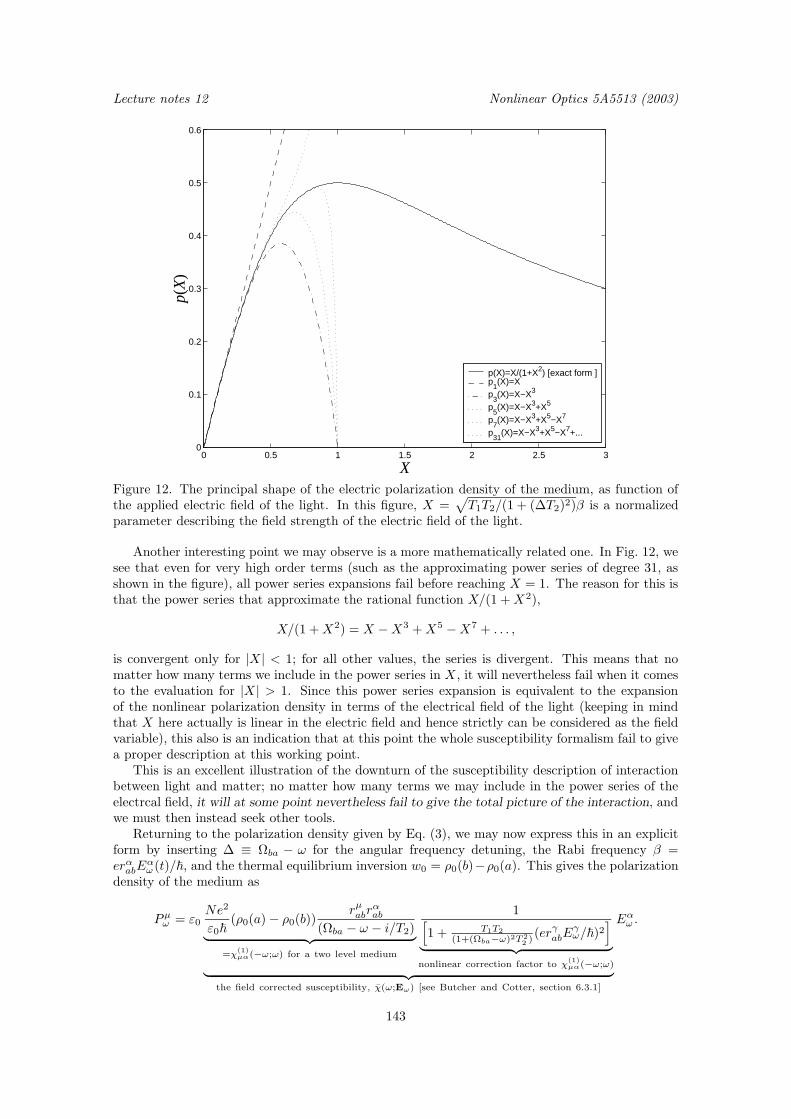
Lecture notes 12 Nonlinear Optics 5A5513 (2003)
0 0.5 1 1.5 2 2.5 30
0.1
0.2
0.3
0.4
0.5
0.6
X
p(X
)
p(X)=X/(1+X2) [exact form ] p
1(X)=X
p3(X)=X−X3
p5(X)=X−X3+X5
p7(X)=X−X3+X5−X7
p31
(X)=X−X3+X5−X7+...
Figure 12. The principal shape of the electric polarization density of the medium, as function ofthe applied electric field of the light. In this figure, X =
√T1T2/(1 + (∆T2)2)β is a normalized
parameter describing the field strength of the electric field of the light.
Another interesting point we may observe is a more mathematically related one. In Fig. 12, wesee that even for very high order terms (such as the approximating power series of degree 31, asshown in the figure), all power series expansions fail before reaching X = 1. The reason for this isthat the power series that approximate the rational function X/(1 +X2),
X/(1 +X2) = X −X3 +X5 −X7 + . . . ,
is convergent only for |X| < 1; for all other values, the series is divergent. This means that nomatter how many terms we include in the power series in X, it will nevertheless fail when it comesto the evaluation for |X| > 1. Since this power series expansion is equivalent to the expansionof the nonlinear polarization density in terms of the electrical field of the light (keeping in mindthat X here actually is linear in the electric field and hence strictly can be considered as the fieldvariable), this also is an indication that at this point the whole susceptibility formalism fail to givea proper description at this working point.
This is an excellent illustration of the downturn of the susceptibility description of interactionbetween light and matter; no matter how many terms we may include in the power series of theelectrcal field, it will at some point nevertheless fail to give the total picture of the interaction, andwe must then instead seek other tools.
Returning to the polarization density given by Eq. (3), we may now express this in an explicitform by inserting ∆ ≡ Ωba − ω for the angular frequency detuning, the Rabi frequency β =erαabE
αω (t)/~, and the thermal equilibrium inversion w0 = ρ0(b)−ρ0(a). This gives the polarization
density of the medium as
Pµω = ε0Ne2
ε0~(ρ0(a) − ρ0(b))
rµabrαab
(Ωba − ω − i/T2)︸ ︷︷ ︸=χ
(1)µα(−ω;ω) for a two level medium
1[1 + T1T2
(1+(Ωba−ω)2T 22 )
(erγabEγω/~)2
]
︸ ︷︷ ︸nonlinear correction factor to χ
(1)µα(−ω;ω)
︸ ︷︷ ︸the field corrected susceptibility, χ(ω;Eω) [see Butcher and Cotter, section 6.3.1]
Eαω .
143

Nonlinear Optics 5A5513 (2003) Lecture notes 12
In this form, the polarization density is given as the product with a term which is identical to thelinear susceptibility4 (as obtained in the perturbation analysis in the frame of the susceptibilityformalism), and a correction factor which is a nonlinear function of the electric field.
The nonlinear correction factor, of the form 1/(1 + X2), with X =√T1T2/(1 + (∆T2)2)β as
previously, can now be expanded in a power series around the small-signal limit X = 0, using
1/(1 +X2) = 1 −X2 +X4 −X6 + . . . ,
from which we obtain the polarization density as a power series in the electric field (which for thesake of simplicitly now is taken as linearly polarized along the x-axis) as
P xω ≈ ε0Ne2
ε0~(ρ0(a) − ρ0(b))
rxabrxab
(Ωba − ω − i/T2)Exω
− ε0Ne4
ε0~3(ρ0(a) − ρ0(b))
rxabrxab
(Ωba − ω − i/T2)
(rxab)2
[1/T 22 + (Ωba − ω)2](T2/T1)
|Exω|2Exω
+ ε0Ne6
ε0~5(ρ0(a) − ρ0(b))
rxabrxab
(Ωba − ω − i/T2)
(rxab)4
[1/T 22 + (Ωba − ω)2]2(T2/T1)2
|Exω|4Exω
+ . . .
(5)
This form is identical to one as obtained in the susceptibility formalism; however, the steps thatled us to this expression for the polarization density do not rely on the perturbation theory ofthe density operator, but rather on the explicit form of the steady-state solutions to the Blochequations.
Summary of the Bloch and susceptibility polarization densities
To summarize this last lecture on the Bloch equations, expressing the involved parameters in thesame style as previously used in the description of the susceptibility formalism, the polarizationdensity obtained from the steady-state solutions to the Bloch equations is
Pµω = ε0Ne2
ε0~(ρ0(a) − ρ0(b))
rµabrαab
(Ωba − ω − i/T2)
1[1 + T1T2
(1+(Ωba−ω)2T 22 )
(erαabEαω/~)2
]Eαω .
By expanding this in a power series in the electrical field, one obtains the form (5), in which wefrom the same description of the polarization density in the susceptibility formalism can identify
χ(1)xx (−ω;ω) =
Ne2
ε0~(ρ0(a) − ρ0(b))
rxabrxab
(Ωba − ω − i/T2),
χ(3)xxxx(−ω;ω, ω,−ω) = − 4Ne4
3ε0~3(ρ0(a) − ρ0(b))
rxabrxab
(Ωba − ω − i/T2)
(rxab)2
[1/T 22 + (Ωba − ω)2](T2/T1)
,
χ(5)xxxxxx(−ω;ω, ω,−ω,ω,−ω)
=8Ne6
5ε0~5(ρ0(a) − ρ0(b))
rxabrxab
(Ωba − ω − i/T2)
(rxab)4
[1/T 22 + (Ωba − ω)2]2(T2/T1)2
,
as being the first contributions to the two-level polarization density, including up to fifth orderinteractions. For a summary of the non-resonant forms of the susceptibilities of two-level systems,se Butcher and Cotter, Eqs. (6.71)–(6.73).
4 In the explicit expressions for the linear susceptibility, for example Butcher and Cotter’sEqs. (4.58) and (4.111) for the non-resonant and resonant cases, respectively, there are two terms,one with Ωba − ω in the denominator and the other one with Ωba + ω. The reason why the secondform does not appear in the expression for the field corrected susceptibility, as derived from theBloch equations, is that we have used the rotating wave approximation in the derivation of thefinal expression. (Recapitulate that in the rotating wave approximation, terms with oscillatory de-pendence of exp[i(Ωba + ω)t] were neglected.) As a result, all temporally phase-mismatched termsare neglected, and in particular only terms with Ωba − ω in the denominator will remain. This,however, is a most acceptable approximation, especially when it comes to resonant interactions,where terms with Ωba − ω in the denominator by far will dominate over non-resonant terms.
144

Lecture notes 12 Nonlinear Optics 5A5513 (2003)
Appendix: Notes on the numerical solution to the Bloch equations
In their original form, the Bloch equations for a two-level system are given by Eqs. (1) as
du
dt= −∆v − u/T2,
dv
dt= ∆u+ β(t)w − v/T2,
dw
dt= −β(t)v − (w − w0)/T1.
By taking the time in units of the transverse relaxation time T2, as
τ = t/T2,
the Bloch equations in this normalized time scale become
du
dτ= −∆T2v − u,
dv
dτ= ∆T2u+ β(t)T2w − v,
dw
dτ= −β(t)T2v − (w − w0)T2/T1.
In this system of equations, all coefficients are now normalized and physically dimensionless, ex-pressed as relevant quotes between relaxation times and products of the Rabi frequency or detuningfrequency with the transverse relaxation time. Hence, by taking the normalized parameters
δ = ∆T2,
γ(t) = β(t)T2,
η = T1/T2,
where δ can be considered as the normalized detuning from molecular resonance of the medium,γ(t) as the normalized Rabi frequency, and η as a parameter which describes the relative impactof the longitudinal vs transverse relaxation times, the Bloch equations take the normalized finalform
du
dτ= −δv − u,
dv
dτ= δu+ γ(t)w − v,
dw
dτ= −γ(t)v − (w − w0)/η.
This normalized form of the Bloch equations has been used throughout the generation of graphsin Figs. 2–11 of this lecture, describing the qualitative impact of different regimes of resonance andrelaxation. The normalized Bloch equations were in the simulations shown in Figs. 2–11 integratedby using the standard routine ODE45() in MATLAB.
145

Nonlinear Optics 5A5513 (2003) Lecture notes 12
146

Lecture Notes on Nonlinear Optics Nonlinear Optics 5A5513 (2003)
Home Assignments
147

Nonlinear Optics 5A5513 (2003) Lecture Notes on Nonlinear Optics
Lecture Notes on Nonlinear OpticsNonlinear Optics (5A5513, 5p for advanced undergraduate and doctoral students)Course given at the Royal Institute of Technology,Department of Laser Physics and Quantum OpticsSE–106 91, Stockholm, SwedenJanuary 8 – March 24, 2003
The texts and figures in this lecture series was typeset by the author in 10/12/16 pt ComputerModern typeface using plain TEX and METAPOST.
This document is electronically available at the homepage of the Library of the Royal Institute ofTechnology, at http://www.lib.kth.se.
Copyright c© Fredrik Jonsson 2003
All rights reserved. No part of this publication may be reproduced, stored in a retrieval system,or transmitted, in any form, or by any means, electronic, mechanical, photo-copying, recording, orotherwise, without the prior consent of the author.
ISBN 91-7283-517-6TRITA-FYS 2003:26ISSN 0280-316XISRN KTH/FYS/- - 03:26 - - SEPrinted on July 7, 2003
TEX is a trademark of the American Mathematical Society
148
Nonlinear Optics 5A5513 (2003)
Home Assignments
The assignments are of various algebra-intense degrees, and they are not listed in any order oflevel of difficulty. Solutions to the assignments by means of MapleV, Mathematica, or any otherprograms for symbolic analysis is encouraged. In the assignments, any reference to “Butcher andCotter’s book” should be read as “P. N. Butcher and D. Cotter, The Elements of Nonlinear Optics(Cambridge University Press, Cambridge, 1991), ISBN 0-521-42424-0”.
The assignments give a total maximum of 44.0 marks, and successful examination is guaranteedat fifty percent of this level, or 22.0 marks.
Solutions to the assignments should be handed in no later than April 22, 2003, to Fredrik Laurellor Jens Tellefsen, at the department of Laser Physics and Quantum Optics, KTH, Roslagstulls-backen 21, Albanova Universitetscentrum (Fysikcentrum), SE-106 91, Stockholm.
Questions regarding the assignments can be directed to the lecturer and examiner Fredrik Jonsson,preferrably via email to [email protected].
149

Nonlinear Optics 5A5513 (2003)
[This page is intentionally left blank]
150
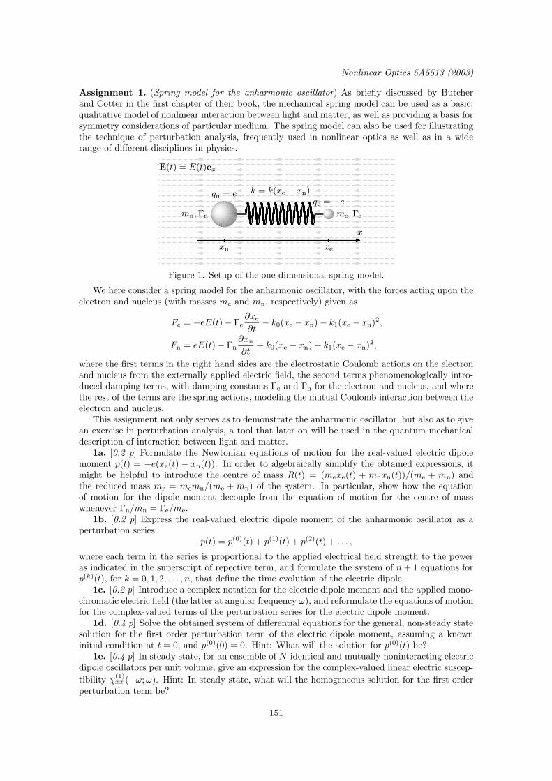
Nonlinear Optics 5A5513 (2003)
Assignment 1. (Spring model for the anharmonic oscillator) As briefly discussed by Butcherand Cotter in the first chapter of their book, the mechanical spring model can be used as a basic,qualitative model of nonlinear interaction between light and matter, as well as providing a basis forsymmetry considerations of particular medium. The spring model can also be used for illustratingthe technique of perturbation analysis, frequently used in nonlinear optics as well as in a widerange of different disciplines in physics.
E(t) = E(t)ex
x
xn
mn,Γn
qn = e
xe
me,Γe
qe = −ek = k(xe − xn)
Figure 1. Setup of the one-dimensional spring model.
We here consider a spring model for the anharmonic oscillator, with the forces acting upon theelectron and nucleus (with masses me and mn, respectively) given as
Fe = −eE(t) − Γe∂xe
∂t− k0(xe − xn) − k1(xe − xn)2,
Fn = eE(t) − Γn∂xn
∂t+ k0(xe − xn) + k1(xe − xn)2,
where the first terms in the right hand sides are the electrostatic Coulomb actions on the electronand nucleus from the externally applied electric field, the second terms phenomenologically intro-duced damping terms, with damping constants Γe and Γn for the electron and nucleus, and wherethe rest of the terms are the spring actions, modeling the mutual Coulomb interaction between theelectron and nucleus.
This assignment not only serves as to demonstrate the anharmonic oscillator, but also as to givean exercise in perturbation analysis, a tool that later on will be used in the quantum mechanicaldescription of interaction between light and matter.
1a. [0.2 p] Formulate the Newtonian equations of motion for the real-valued electric dipolemoment p(t) = −e(xe(t) − xn(t)). In order to algebraically simplify the obtained expressions, itmight be helpful to introduce the centre of mass R(t) = (mexe(t) + mnxn(t))/(me + mn) andthe reduced mass mr = memn/(me + mn) of the system. In particular, show how the equationof motion for the dipole moment decouple from the equation of motion for the centre of masswhenever Γn/mn = Γe/me.
1b. [0.2 p] Express the real-valued electric dipole moment of the anharmonic oscillator as aperturbation series
p(t) = p(0)(t) + p(1)(t) + p(2)(t) + . . . ,
where each term in the series is proportional to the applied electrical field strength to the poweras indicated in the superscript of repective term, and formulate the system of n+ 1 equations forp(k)(t), for k = 0, 1, 2, . . . , n, that define the time evolution of the electric dipole.
1c. [0.2 p] Introduce a complex notation for the electric dipole moment and the applied mono-chromatic electric field (the latter at angular frequency ω), and reformulate the equations of motionfor the complex-valued terms of the perturbation series for the electric dipole moment.
1d. [0.4 p] Solve the obtained system of differential equations for the general, non-steady statesolution for the first order perturbation term of the electric dipole moment, assuming a knowninitial condition at t = 0, and p(0)(0) = 0. Hint: What will the solution for p(0)(t) be?
1e. [0.4 p] In steady state, for an ensemble of N identical and mutually noninteracting electricdipole oscillators per unit volume, give an expression for the complex-valued linear electric suscep-
tibility χ(1)xx (−ω;ω). Hint: In steady state, what will the homogeneous solution for the first order
perturbation term be?
151

Nonlinear Optics 5A5513 (2003)
1f. [0.2 p] In steady state, give an expression for the dispersion ∂n(ω)/∂ω.1g. [0.4 p] In steady state, still for an ensemble of N identical and mutually noninteracting
electric dipole oscillators per unit volume, give expressions for the complex-valued second-order
electric susceptibilities χ(2)xxx(−2ω;ω, ω) and χ
(2)xxx(0;ω,−ω).
1h. [0.4 p] Can the quadratic term in the expression for the spring action cause the (third-order) optical Kerr-effect, that is to say, can it give rise to a nonzero electric dipolar susceptibility
χ(3)xxxx(−ω;ω, ω,−ω)?
1i. [0.3 p] Can the quadratic term in the expression for the spring action cause the (third-order) effect of optical third harmonic generation, that is to say, can it give rise to a nonzero
electric dipolar susceptibility χ(3)xxxx(−3ω;ω, ω, ω)?
1j. [0.4 p] If cubic terms ±k2(xe − xn)3 were to be included in the expression for the springaction on the electron and nucleus, respectively, would these terms be able to induce an additionalcomponent at angular frequency 2ω?
1k. [0.3 p] If cubic terms ±k2(xe − xn)3 were to be included in the expression for the springaction on the electron and nucleus, respectively, would these terms be able to cause optical Kerr-effect?
Assignment 2. (Review of quantum mechanics – The density matrix) While the mechanical springmodel provides a qualitative picture that for many cases is sufficcient, it nevertheless fails to give aproper basis for a description of interaction between light and matter down to the molecular level.The aim with this assignment is to provide a summary of the maybe somewhat abstract (butnecessary) quantum mechanical tools that are needed for the description of interaction betweenlight and matter.
This assignment virtually covers all the quantum mechanics needed for understanding the basisof the nonlinear optics described in this course, and it also demonstrates the point in nonlinearoptics at which we choose either to proceed with perturbation analysis of the matrix elements ofthe density operator (introducing the nonlinear susceptibility formalism), or to solve for the matrixelements directly by instead using the Bloch equation.
2a. [2.5 p] Starting from the time dependent Schrodinger equation for the molecular wave func-tion, derive the equation of motion for the density matrix in the Schrodinger picture. In Butcherand Cotters book, this corresponds to filling in the details in the discussion from Eq. (3.1) toEq. (3.50). (This may sound like a formidable task of deriving fifty quantum mechanical equa-tions; however, most of these equations are simple definitions and corollaries, and by followingthe outline as described in Butcher and Cotters book, this is quite a straightforward task whichhopefully will give a deeper understanding of the origin of optical nonlinearities.)
2b. [1.0 p] Starting from the equation of motion for the density matrix in the Schrodingerpicture, apply perturbation analysis and derive the general solution for the nth order term of thedensity operator. In Butcher and Cotters book, this corresponds to filling in the details in thediscussion from Eq. (3.50) to Eq. (3.82).
2c. [0.4 p] In your own words, explain the difference between the “Schrodinger picture” and“interaction picture” in quantum mechanics.
Assignment 3. (Nonlinear optics of the hydrogen atom) Among the simplest systems that arepossible to analyse analytically, the hydrogen and helium atoms serve as to give models for nonlinearoptical effects. In this assignment, the task is to essentially to perform the calculations necessaryfor predicting the refractive index and optical Kerr-effect of hydrogen gas. However, in order tosimplify the task, we will instead perform the calculations for an ensemble of hydrogen atoms,rather than for the in nature commonly appearing diatomic H2 molecules. This assumption makesthis assignment a somewhat artificial construction, which though nevertheless serve well as toillustrate the steps leading from the atomic wavefunction (or molecular wavefunction, if we wereto consider a “real” gas of H2 molecules) to the concept of linear refractive index (given by thefirst order electric susceptibility) and optical Kerr-effect.
152

Nonlinear Optics 5A5513 (2003)
The wave function of the hydrogen atom is in spherical coordinates (r, ϕ, ϑ) given as [H. Hakenand H. C. Wolf, The physics of atoms and quanta, 4th ed. (Springer-Verlag, Berlin, 1993)]
ψnlm(r, ϑ, ϕ) = Rnl(r)Pml (cosϑ) exp(imϕ),
where n is the principal quantum number, l the angular momentum quantum number, and m themagnetic quantum number or directional quantum number. These numbers assume the values
n = 1, 2, . . . , 0 ≤ l ≤ n− 1, −l ≤ m ≤ l.
In the angular part of the expression for the wave function,
P 0l (ξ) = Pl(ξ) =
1
l!2ldl
dξl(ξ2 − 1)l
are the Legendre polynomials, and
Pml (ξ) = (1 − ξ2)m/2dm
dξmPl(ξ)
are the associated Legendre functions, while for the radial part
Rnl(r) = Nnl exp(−κnr)rlL2l+1n+1 (2κnr),
where Nnl is a normalization constant obtained from the condition
∫ ∞
0
R2nl(r)r
2 dr = 1,
and
κn =
(m0Ze
2
~24πε0
)1
n.
Above L2l+1n+1 are the Laguerre function of the second kind, obtained from the Laguerre polynomials
through 2l + 1-fold differentiation
L2l+1n+1 (ξ) =
d2l+1
dξ2l+1Ln+1(ξ).
The temperature of the (artificial) hydrogen gas here condidered is 25 degrees Celcius, measuredat 1077 mBar pressure, and it is reasonable to assume that the hydrogen atoms in the ensembleare mutually noninteracting.
3a. [1.0 p] Calculate the first order electric dipolar susceptibility χ(1)µα(−ω;ω) and the linear
refractive index n(ω), for a vacuum wavelength of 580 nm. Hint: Consider hydrogen being in theground state and identify the atomic trasition frequencies closest to the frequency range of interest.Is it likely that resonant interaction should be taken into account?
3b. [1.0 p] Calculate the second order electric dipolar susceptibility χ(2)µαβ(−2ω;ω, ω), for the
same vacuum wavelength as in assignment 3a.
3c. [1.0 p] Calculate the third order electric dipolar susceptibility χ(3)µαβγ(−ω;ω, ω,−ω), for the
same vacuum wavelength as in assignment 3a.3d. [0.2 p] Would you a priori (i. e. without actually performing the calculations) expect the
elements of the linear susceptibility tensor χ(1)µα(−ω;ω) to be lower or higher for an ensemble of
helium atoms than for the ensemble of hydrogen atoms?3e. [0.2 p] Would you a priori expect the elements of the quadratic susceptibility tensor
χ(2)µαβ(−2ω;ω, ω) to be lower or higher for an ensemble of helium atoms than for the ensemble
of hydrogen atoms?
153

Nonlinear Optics 5A5513 (2003)
Assignment 4. (Neumann’s principle in linear optics) Being a powerful tool in a variety of disci-plines in physics, Neumann’s principle simply states that any type of symmetry which is exhibitedby the point symmetry group of the medium also is possessed by every physical property of themedium.
In many textbooks in linear optics and electromagnetic wave propagation, it is taken more orless as an axiom that the linear susceptibility tensors of cubic media are diagonal with all elementsequal, i. e. in form identical to the linear susceptibility tensor of isotropic media. However, onerarely finds a strict derivation of this fact, and since Neumann’s principle is a powerful tool innonlinear optics, this assignment serves as an introduction to analysis of point symmetries ofhigher order, nonlinear interactions.
4a. [0.2 p] Is an isotropic medium always centrosymmetric, that is to say, does it always possessa center of inversion? (This question is of a general character, and applies to linear as well asnonlinear optical regimes.)
4b. [0.2 p] Is a centrosymmetric medium always isotropic?
4c. [0.8 p] Show that the electric dipolar susceptibility tensor χ(1)µα(−ω;ω) takes the form
χ(1)xx (−ω;ω)δµα for a medium belonging to cubic point-symmetry class.
4d. [0.8 p] In addition, show that the susceptibility tensor χ(1)xx (−ω;ω)δµα also is isotropic,
i. e. that it in fact is left invariant under any rotation of the cordinate axes of the medium.
4e. [0.8 p] Show that the electric dipolar susceptibility tensor χ(1)µα = χ
(1)µα(−ω;ω) takes the
form
χ(1)(−ω;ω) =
χ
(1)xx 0 0
0 χ(1)xx 0
0 0 χ(1)zz
for trigonal media.
Assignment 5. (Neumann’s principle in nonlinear optics) As shown in the course, the principlesfor reduction of the elements of first-order susceptibility tensors by means of direct inspection caneasily be extended and applied to susceptibilities describing nonlinear interactions as well.
While, for example, media belonging to the cubic crystallographic point symmetry group allbehave as isotropic in linear optics, they will in the nonlinear optical regime generally be of non-isotropic character. In addition, calculations of symmetry properties of higher-order susceptibilitiestend to be less intuitive than in linear optics. However, Neumann’s principle, together with thetransformation properties of polar tensors (such as electric dipolar susceptibilities), provides apowerful tool that is well suited for implementation in computer languages for symbolic analysis,significantly reducing the effort needed for solving the problems.
5a. [0.4 p] Within the electric dipole approximation, the linear susceptibility tensor of isotrop-ic media is always diagonal with all elements equal (as, hopefully, also shown in assignment 5),hence preventing any coupling between polarization states. Is it true that no such polarizationstate coupling appears in isotropic media in the nonlinear optical regime as well? Prove or give acounterexample!
5b. [0.3 p] Prove that the elements of χ(2n)µα1···α2n
(−ωσ;ω1, . . . , ω2n) are all identically zero formedia possessing a center of inversion, for n being a positive integer.
5c. [0.6 p] In Fig. 2, objects possessing the point symmetry properties of crystallographic cubicpoint symmetry classes 432, m3, 43m, and 23 are shown [N. W. Ashcroft and N. D. Mermin, Solidstate physics (Saunders College Publishing, Orlando, 1976)].
The description of the objects is closed by the observation that the objects of these pointsymmetry classes all should be left invariant under any ±120 degrees rotation around any spacediagonal axis, going through diametrically opposite corners.
Without entering any calculations, is it possible to immediately tell which of those point sym-metry classes that will lead to an identically zero second order electric dipolar susceptibility?Motivate with a few figures!
154

Nonlinear Optics 5A5513 (2003)
2/m, 3 (m3) 432
43m 23
Figure 2. Objects possessing the point symmetry properties of 432, m3, 43m, and 23.
5d. [1.0 p] For any of the point symmetry groups 432, m3, 43m, or 23 that possesses anonzero second order susceptibility, derive the set of nonzero and independent tensor elements
of χ(2)µαβ(−ωσ;ω1, ω2).5e. [0.6 p] For a light beam propagating in the z-direction, will any of the point symmetry
groups 432, m3, 43m, or 23 give a second order polarization density that is left invariant underrotation of the medium around the z-axis? (Of course under the assumption that the optical waveproperties, such as the polarization state of the wave, are kept fixed in space under the rotation.)
5f. [0.6 p] Prove that in isotropic media
χ(3)xxxx = χ(3)
xxyy + χ(3)xyxy + χ(3)
xyyx,
for arbitrary frequency arguments.5g. [0.6 p] As listed in Appendix 3 of Butcher and Cotter’s book (and as also is straightforward
to verify by applying Neumann’s principle and the technique of direct inspection, as in assignment5f above), the general third-order electric dipolar susceptibility of isotropic media, for arbitraryfrequency arguments, possesses the property
χ(3)xxxx = χ(3)
xxyy + χ(3)xyxy + χ(3)
xyyx,
that is to say, the xxxx-element equals to the sum of the (three) distinct permutations of thetensor elements with x in the first index, and with equal total number of x and y appearing in theindices. As a generalization of this relation, one may hence expect the fifth-order susceptibility ofisotropic media, again for arbitrary frequency arguments, to possess the property
χ(5)xxxxxx = χ(5)
xxxyyy + χ(5)xxyxyy + χ(5)
xxyyxy
+ χ(5)xxyyyx + χ(5)
xyxxyy + χ(5)xyxyxy
+ χ(5)xyxyyx + χ(5)
xyyxxy + χ(5)xyyxyx + χ(5)
xyyyxx,
that is to say, suggesting that the xxxxxx-element equals to the sum of the (ten) distinct permu-tations of the tensor elements with x in the first index, and with equal total number of x and yappearing in the indices. The question is: Is the above statement for the fifth order susceptibilityreally true?
155

Nonlinear Optics 5A5513 (2003)
Assignment 6. (Review of quantum mechanics – The resonant two-level system) In assignment 2,the analysis of the density operator is performed essentially under the assumption of nonresonantinteraction between light and matter, even though the principles of perturbation analysis applyto weakly resonant systems as well. For strongly resonant interactions, the higher order perturba-tion terms can no longer be considered as small compared to lower order ones, and eventually adescription in terms of the susceptibility formalism fails to give a proper picture. For such cases,the density operator is instead described by Bloch-type equations, which when solved provide theobservable, macroscopic properties of the medium by evaluation of quantum-mechanical traces.
The outline for this technique, as in this assignment described for the two-level system, canequally well be applied to n-level systems as well, though with an increasing algebraic complexity.
6a. [1.6 p] Starting from the time dependent Schrodinger equation for the two-level molecularwave function, derive the Bloch equations in the rotating-wave approximation. In Butcher andCotters book, this corresponds to filling in the details in the discussion from Eq. (6.22) to Eq. (6.52).
6b. [0.4 p] Can the rotating wave approximation be considered as a kind of phase matching,similar to the phase matching conditions that frequently appear elsewhere in nonlinear optics?Motivate.
Assignment 7. (Nonlinear optics of silica) In the wavelength range from ultraviolet to mid-infrared, the Sellmeier expression for the linear, field-independent refractive index n(λ) of puresilica (SiO2, quartz) is given as
n2(λ) = 1 +
3∑
k=1
Akλ2
λ2 − λ2k
,
where λ is the vacuum wavelength of the light, and where the physically dimensionless constantsAk are experimentally found to be
A1 = 0.6961663, A2 = 0.4079426, A3 = 0.8974794.
The resonance vacuum wavelengths in the Sellmeier expression are for silica given as
λ1 = 0.0684043µm, λ2 = 0.1162414 µm, λ3 = 9.896161 µm,
where λ1 and λ2 are electronic resonances, and λ3 a lattice vibrational resonance.
7a. [0.4 p] Using the Sellmeier expression, give an expression for the χ(1)αβ(−ω;ω) in terms of the
parameters Ak and λk. You may here assume the silica to be essentially isotropic. (This assumptionholds for amorphous SiO2, but it should be emphasized that this approximation in general doesnot hold for quartz in a pure crystalline (trigonal) state, which belongs to the crystallographicpoint symmetry class 32.)
7b. [0.2 p] In the visible range, say at vacuum wavelength 700 nm, calculate the relative con-tribution from the vibrational term to the index of refraction.
7c. [0.6 p] Using the obtained expression for χ(1)αβ(−ω;ω), identify and express the magnitudes
|erαab| of the corresponding matrix elements of the electric dipole moments, in terms of the λk andAk parameters of the Sellmeier expression. Calculate the numerical values of |erαab| in regular SIunits. You may assume that (I) the SiO2 molecules are in the ground state, and that (II) the latticevibrational contribution safely can be neglected in comparison with the electronic contributions.
7d. [0.4 p] Having obtained the magnitudes of the matrix elements of the involved electricdipole moments of quartz, apply the Unsold approximation in order to obtain a simplified, effectiveexpression for the refractive index of the form
n2eff(λ) = 1 +
Aeffλ2
λ2 − λ2eff
,
where the task now is to find expressions for Aeff and λeff . Also find the maximum deviation ofthe obtained refractive index from the one given by the original Sellmeier expression, taken overthe vacuum wavelength interval from 400 nm to 870 nm.
7e. [0.8 p] Make use of the obtained expressions of the matrix elements of the involved electricdipole moments of quartz to calculate an approximative value of the third-order susceptibility
χ(3)xxxx(−ω;ω, ω,−ω), taken over the same vacuum wavelength interval as in assignment 7d.
156
Nonlinear Optics 5A5513 (2003)
Assignment 8. (The Bloch equation) Suppose a Mg26 atom is trapped and excited with a laserbeam tuned close to the 3s2 1S0–3s3p
1P1 transition (with the angular frequency of the laser lighttaken as ω = ω3s3p 1P1
−ω3s2 1S0+∆ω). Suppose the atom can be considered as a two-level system,
and that the excitation hence can be described by the Bloch equations for a two-level system. Theenergy level for the 3s3p 1P1 state of Mg26 is 35051 cm−1. (See, for example, Atomic Energy Levels,National Bureau of Standards, Circular 467.)
8a. [1.0 p] For a circular laser beam of 1 mm radius, with top-hat profile, calculate at whichoptical power the Rabi angular frequency Ω equals to Ω = 1/(3τ), where τ = 2 ns is the life timeof the 3s3p 1P1 state of Mg26.
8b. [0.8 p] Calculate the probability that the atom is in the upper state for ∆ω = 0 and∆ω = 1/τ , for steady state between the optical field and relaxation processes.
Hint: Do not start the calculations until you have made it clear in which way the assumptionof steady state simplifies the problem.
Assignment 9. (Vector model for the Bloch equation) The time dependent solution to the Blochequations for an optical field tuned to exact resonance, when the electromagnetic field and thenatural life time are the only broadening mechanisms, and with the initial values u(0) = v(0) = 0and w(0) = −1, are
u(t) = 0,
v(t) =2ΩT2
2 + (ΩT2)2
[cos(βt) +
1 − (ΩT2)2
2βT2sin(βt)
]exp(−3t/2T2) − 1
,
w(t) =(ΩT2)
2
2 + (ΩT2)2
1 −
[cos(βt) +
3
2βT2sin(βt)
]exp(−3t/2T2)
− 1,
with β = [Ω2 − 1/(4T 22 )]1/2. Now suppose that Mg26 is contained in a cell at 200 degrees Celsius.
Choose ∆ω = 0 and an optical intensity such that ΩT2 = 5.9a. [0.7 p] As the optical field is switched on, the atoms of the Mg26 sample are excited to the
upper level. As the Bloch vector rotates, the population in the upper state will at some time T0
start to decrease again. Calculate the time T0 and the population density ρ22(T0) at this time.9b. [1.0 p] Calculate the length of the cell in order for the incindent optical intensity to decrease
by 10 percent at t = T0. The energy emitted by spontaneous emission is here neglected forsimplicity, as in 9c.
9c. [0.7 p] Calculate ρ22(2T0) and the relative amount of the incident light energy that hasbeen absorbed at t = 2T0. If the system had been undamped, how much of the light would thenhave been absorbed after the Bloch vector had rotated one turn?
9d. [1.0 p] Draw approximately how the Bloch vector evolve, from the time at which the lightis switched on until steady state is reached, and how it then evolves as the light is switched offagain.
157

Nonlinear Optics 5A5513 (2003)
Assignment 10. (Optical bistability) As a medium possessing optical Kerr-effect is placed insidea cavity, either in a ring cavity (in which only unidirectional wave propagation is considered) or ina Fabry-Perot cavity (in which counter-propagating waves may couple as well), one introduces anoptical feedback to the nonlinear interaction between light and matter. For certain configurationsthis feedback leads to phenomena where the system is latched into stable states, in particularwith the transmitted intensity taking two possible stable values for a given input, so-called opticalbistability, where the two states of the system can be pictured as “low” (switched off) and “high”(switched on).
optical Kerr medium
L
|ρb|2 = 1 |ρb|2 = 1
ρa ρaEIω ET
ω
Figure 3. Setup of the ring cavity for optical bistability.
optical Kerr medium
L
ρa ρa
EIω ET
ω
Figure 4. Setup of the Fabry-Perot cavity for optical bistability.
10a. [1.0 p] For the ring cavity configuration, using an all-dispersive isotropic optical Kerr-medium, formulate the equation that relates the transmitted intensity IT = (ε0c/2)|ET
ω |2 to theincident intensity II = (ε0c/2)|EI
ω|2. In the ring cavity configuration, the two semitransparentmirrors are assumed to have a complex amplitude reflectance of ρa each, while the rest of themirrors have a reflectance of unity. For simplicity, you may neglect the reflectance of the opticalbeam at the end surfaces of the nonlinear medium, hence neglecting any back-reflected wave in thering cavity. You may also assume the light to be linearly polarized (TE or TM with respect to theplane of incidence on the mirrors), enabling a scalar theory of wave propagation to be applicableto the problem.
10b. [1.0 p] Same as 10a, but now for the Fabry-Perot cavity configuration, where the nonlinearmedium is enclosed by two mirrors of complex amplitude reflectance ρa.
10c. [0.4 p] For the ring cavity or the Fabry-Perot cavity configuration (your choice), explainhow the obtained relations between transmitted and incindent intensities lead to optical bistability.
10d. [0.4 p] In purely dispersive optical bistability, for which there is no absorption, whathappens to the light energy contained in the cavity as the system switches from the upper to thelower state of transmission?
158
Nonlinear Optics 5A5513 (2003)
Instead of solving the above problems, you may solve one of the following two additional problemson optical bistability:
10′. [2.8 p] Formulate the equation for absorptive optical bistability with an inhomogeneouslybroadened isotropic two-level medium. Prove that this equation can (or cannot) exhibit opticalbistability.
10′′. [2.8 p] Compare and contrast absorptive and dispersive optical bistability for isotropicmedia. How are the incident and transmitted field phases related for each case?
Assignment 11. (Optical solitons) As shown in the course, optical solitons are solutions to thewave equation in optical Kerr-media, where the intensity-dependent refractive index of the mediumbalance the dispersion.
11a. [1.0 p] Prove that for an initial pulse shape given by u(0, s) = N sech(s), with N = 1 forthe fundamental soliton, an exact soliton solution u(ζ, s) to the nonlinear Schrodinger equation isgiven by
u(ζ, s) = sech(s) exp(iζ/2).
11b. [0.4 p] For quartz, the numerical value of the xyyx element of the nonlinear susceptibilityis given as
χ(3)xyyx(−ω;ω, ω,−ω) = 8.0 × 10⁻²³ m2/V2,
at a vacuum wavelength of 1 694 nm. Calculate the numerical values of χ(3)xxxx(−ω;ω, ω,−ω) and
the nonlinear refractive index n2 at this vacuum wavelength. Hint: Consider Kleinman symmetryto hold.
11c. [0.6 p] Suggest pulse duration time and peak intensity of an optical pulse at 1 694 nmvacuum wavelength in order to form a fundamental soliton in quartz. Hint: The linear opticalproperties of quartz at this wavelength may, for example, be obtained from the Sellmeier expressiongiven in assignment 7.
Assignment 12. (Third harmonic generation in isotropic media) In this assignment, the task isto formulate the theory of third harmonic generation, in similar to the second harmonic generationanalyzed in the lectures. While second harmonic generation requires the medium to be non-centrosymmetric (if the medium is centrosymmetric, the second order susceptibility is zero, asshown in the lectures), the third harmonic generation does not have this constraint. In particular,we will in this assignment consider the third harmonic generation in isotropic media.
Note that even though this problem concerns isotropic media, the third harmonic signal ishighly dependent on the polarization state of the pump wave. As an example, circularly polarizedlight cannot be used for third harmonic generation in isotropic media. (This is, for example, shownin section 5.3.4, page 144, of Butcher and Cotter’s The Elements of Nonlinear Optics.)
This assignment serves as an illustration of a general scheme for solving wave propagationproblems in nonlinear optics, as well as an example of the application of the Butcher and Cotterconvention of degeneracy factors in nonlinear optics. When solving this assignment, you maybenefit from applying the scheme for solving problems in nonlinear optics, as outlined in lecturenine of this course.
12a. [1.0 p] In the infinite plane wave limit, assuming all fields to be polarized in the xy-planeand propagating in the positive z-direction, formulate the polarization density of the isotropicmedium, at the angular frequency ω of the fundamental (pump) wave.
12b. [1.0 p] Using the same assumptions as in 12a, formulate the polarization density at theangular frequency 3ω of the third harmonic wave.
12c. [1.0 p] For a continuous-wave configuration, with the pump wave being linearly polarizedin the x-direction, formulate the coupled system of wave equations for the pump and third harmonicwave. What will the polarization state of the third harmonic wave be?
12d. [1.0 p] Assuming the conversion efficiency from the pump to the third harmonic waveto be small, we may assume the pump wave to be essentially non-depleted, i. e. Aω(z) ≈ const.(non-depleted pump approximation). For this case, derive an expression for the intensity of thethird harmonic wave after a geometrical propagation distance L. (As a hint of the form of thisexpression, you may consult Butcher and Cotter, Eq. (7.30).)
159
Nonlinear Optics 5A5513 (2003)
Assignment 13. (The degeneracy factor) The system of including degenerate terms of the polar-ization density by means of the degeneracy factor K(−ωσ;ω1, . . . , ωn) is very convenient, since it,for example, allow us to use only one of the possible combinations of (ω1, . . . , ωn) for the descriptionof some particular nonlinear interaction, instead of considering all possible permutations. How-ever, the convention of taking the real-valued electrical field as E(r, t) = Re[Eω exp(−iωt)] is notuniversal, and in the 1960’s, the convention was rather to take it as E(r, t) = Eω exp(−iωt) + c. c.,i. e. as twice of the convention of Butcher and Cotter. Sometimes it is though useful to apply the“old” convention, especially if it comes to the interpretation of pioneering publications in the fieldof nonlinear optics.
13a. [3.0 p] Reformulate the degeneracy factor given by Butcher and Cotter, Eq. (2.56), forthe case where the real-valued field instead is taken as E(r, t) = Eω exp(−iωt) + c. c..
13b. [1.0 p] Why would one suspect that a misinterpretation of the convention of the real-valued field has a greater impact in nonlinear optics rather than in linear optics?
160

Nonlinear Optics 5A5513 (2003)
Assignment 14. (Electro-optic phase modulation – The Pockels effect) In this assignment, weconsider an electro-optic light modulator, consisting of a nonlinear optical crystal of litium niobate,LiNbO3, with electrodes plated on the top and bottom surfaces, as shown in Fig. 5. As a DC voltageis applied to the electrodes, the refractive index experienced by the light is changed through thelinear electro-optical Pockels effect, described by the second-order susceptibility
χ(2)µαβ(−ω;ω, 0),
and the resulting phase shift of the light over the crystal can be used in an interferometric setup,for modulation of light intensity.
y
x
z Crystal frame (x, y, z)
LiNbO3
(point symmetry group 3m)
EI(r, t) = Re[Eω exp(−iωt)]= ezRe[Ezω exp(−iωt)]
+
Figure 5. The phase shifting element of the litium niobate electro-optic modulator.
As one example of an interferometric setup in which the phase shift of the light may be detectedas a modulation of intensity is the Mach-Zender configuration, as shown in Fig. 6, where the inputlight waveguide is split into two, with each waveguide now carrying half of the input intensity.A phase shifting electro-optical element is placed in one of the arms of the interferometer (thelower one as shown in Fig. 6), and by modulating the the applied voltage over it, a relative phaseshift between the light in the two arms is obtained. As the two guided light waves are combinedagain, the resulting output will experience either constructive interference (if the relative phaseshift between the beams is a multiple of 2π), or destructive interference (if the phase shift insteadis π plus a multiple of 2π).
Figure 6. The Mach-Zender configuration of an integrated electro-optic modulator.
The task is now to formulate the theory of the basic electro-optic element shown in Fig. 5.14a. [1.0 p] Assuming the applied voltage over the crystal to generate a homogeneous DC
electrical field EzDC in the z-direction, and also assuming the optical field to be linearly polarizedalong the z-direction, propagating in the positive x-direction, formulate the polarization densityat angular frequency ω of the medium.
14b. [1.0 p] For a continuous-wave optical field, formulate the wave equation for the wavepropagation through the medium.
14c. [1.0 p] Solve the wave equation for the envelope of the electrical field. To solve the waveequation, it might be helpful to apply the slowly-varying envelope approximation.
14d. [1.0 p] Formulate the refractive index change of the medium due to the Pockels effect, asfunction of the applied DC electrical field EzDC.
161

Nonlinear Optics 5A5513 (2003)
162
Related Documents