Lecture Notes on Gambling and Risk-Sensitivity

Gambling and Risk-Sensitivity 1

Lecture Notes on Gambling and Risk-SensitivityYakov Ben-Haim

Yitzhak Moda’i Chair in Technology and EconomicsFaculty of Mechanical Engineering

Technion — Israel Institute of TechnologyHaifa 32000 Israel

[email protected]://www.technion.ac.il/yakov

Source material: Yakov Ben-Haim, 2001, 2nd edition, 2006, Information-Gap Decision Theory:

Decisions Under Severe Uncertainty, Academic Press. Chapter 6.

A Note to the Student: These lecture notes are not a substitute for the thorough study of

books. These notes are no more than an aid in following the lectures.

Contents

1 Introduction 2

2 Expected-Utility Risk Aversion 3

3 Preview 5

4 Risk Sensitivity and the Robustness Curve 7

5 Risk Sensitivity and Two Robustness Curves 9

6 Initial Commitment and Uncertain Future 12

6.1 Uniformly Bounded Uncertainty . . . . . . . . . . . . . . . . . . . . . . . . . . 14

6.2 Bounded Fourier Uncertainty . . . . . . . . . . . . . . . . . . . . . . . . . . . 17

7 Risk-Sensitivity, Robustness and Opportuneness 18

8 Risk-Neutral Line 22

9 Pure Competition with Uncertain Cost 26

0lectures\risk\lectures\gambling01.tex 7.2.2006 c⃝ Yakov Ben-Haim 2006.


1 Introduction

¶ The immunity functions,

α(q, rc) β(q, rw) (1)

are the basic decision functions.

However, they:

• Do not determine a decision maker’s choice.

• Do not determine the degree of riskiness of a contemplated action.

¶ Risk (Webster’s):

• “Possibility of loss or injury.

• “Peril”

• “Dangerous element or factor”

• Possible etymology: cliff, rock or submarine hill (Weekley).

• Risk can be quantified in many ways.

• We will consider two approaches:

◦ Assess riskiness of a system.

◦ Assess risk-sensitivity of a decision maker.


2 Expected-Utility Risk Aversion

¶ Consider prizes of value

w1 > w2 > w3 (2)

where

w2 = Pw1 + (1− P )w3 (3)

and 0 < P < 1. These prizes can be won in either of the lotteries:

L : p = (P, 0, 1− P )T (4)

L′ : p ′ = (0, 1, 0)T (5)

P and 1− P are the probabilities of winning w1 and w3 respectively.

L is a gamble between high and low gain.

L′ is a sure bet on an outcome which is the mean of the extremes.

¶ Utility function: u(wi) = decision maker’s personal utility from prize wi.


-

6

Utilityu(w)

Reward, w

w1 w3w2

rruT puT p′

-

6

Utilityu(w)

Reward, w

w1 w3w2

rr uT puT p′

Figure 1: Convex es-timated utility function.Risk proclivity.

Figure 2: Concave es-timated utility function.Risk aversion.

¶ Expected utility of L and L′:

E(L) = Pu(w1) + (1− P )u(w3) = uT p (6)

E(L′) = u(w2) (7)

= u[Pw1 + (1− P )w3] = uT p′ (8)

¶ Expected-utility preference:

L ≻ L′ if and only if Pu(w1) + (1− P )u(w3) > u(w2) (9)

¶ Risk aversion:

• Prefer certainty-equivalent sure thing, w2, over gamble between w1 and w3.

• Prefer L′ over L.

• Fig. 2: Concave utility function.

• Degree of risk aversion: curvature of utility function.

¶ Risk proclivity:

• Prefer gamble between w1 and w3 over certainty-equivalent sure thing, w2.

• Prefer L over L′.

• Fig. 1: Convex utility function.

• Degree of risk proclivity: curvature of utility function.

¶ Expected-utility risk aversion:

• Depends on knowing utilities and probabilities.

• Not usually suited for severe uncertainty.

¶ We will study risk sensitivity from an info-gap perspective.


3 Preview

(Section 6.1)

¶ Tentative and preliminary ideas of info-gap risk:

• Low immunity to failure.

or:

• Limited opportunity for windfall.

¶ Interdependence of risk sensitivity and preferences:

• Risk sensitivity of a decision maker is expressed by choices among options.

• Decision-maker’s choice among options is assisted by interpreting the options in terms of

perceived riskiness.

¶ Risk sensitivity is evaluated by comparing:

what is chosen

against

what could have been chosen

and by evaluating those choices in terms of

robustness and opportuneness.

¶ We will consider 3 types of choices.

1. Given 1 robustness curve, α vs. rc,

where along the curves does the decision maker choose to operate?

This will focus on the robustness premium.

2. Given 2 robustness curves,

• Which is preferred?

• How much reward would the decision maker willingly relinquish to move from one curve

to the other?

This will focus on the robustness premium and the reward premium.

3. Given the alternative between

• Robustness strategy

• Opportuneness strategy

which is preferred?

This will focus on the robustness premium and the opportuneness premium.


¶ Facets of risk sensitivity.

• The profile of:

◦ riskiness

◦ risk sensitivity

will not necessarily be consistent between the 3 approaches.

• They represent different facets of human response to uncertainty, danger, opportunity.


4 Risk Sensitivity and the Robustness Curve

(Section 6.2)

¶ We are familiar with the usual trade-offs:

• α(q, rc) vs. rc.• α(qc(rc), rc) vs. rc.

¶ In the single-robustness-curve context, we assess risk sensitivity in terms of where on the

curve the decision maker chooses to operate, fig. 3.

-

6

rc

α(qc, rc)

rc,1 rc,2 rc,3

s s sriskaverse

riskneutral

riskloving

6

6∆α

∆α′

Figure 3: A robustness curve: robustness versus demanded reward. Illustrating robustness premia,and risk aversion, neutrality and proclivity.

¶ Suppose the decision maker can choose rc:

low reward = rc,1 ≤ rc ≤ rc,3 = high reward (10)

• The decision maker is risk loving if he chooses qc(rc,3):

◦ Demanding maximum available reward.

◦ Relinquishing greatest amount of immunity to uncertainty.

• The decision maker is risk averse if he chooses qc(rc,1):

◦ Demanding maximum available robustness.

◦ Relinquishing greatest amount of reward.

• The decision maker is risk neutral if he chooses qc(rc,2).


¶ What distinguishes these 3 situations is the robustness premium chosen by the DM.

The risk-averse decision maker selects max robustness premium:

∆α = α(qc(rc,1), rc,1)− α(qc(rc,3), rc,3) (11)

in exchange for minimum reward, rc,1.

¶ These concepts of

risk aversion, neutrality, proclivity

make some sense, but they refer to a limited context:

A single robustness curve.

We must consider additional contexts.


-

6

rc

α(qc, rc)

6

6

�

�

r

α1

α2

--

??

α

r1 r2

2

1

demandingmodest

immune

vulnerable

6robustnesspremium

-rewardpremium

α1(qc, rc)

α2(qc, rc)

Figure 4: Maximal robustness versus demanded reward for two alternative options. Illustratingrobustness and reward premia.

5 Risk Sensitivity and Two Robustness Curves

(Section 6.3)

¶ Assess risk-sensitivity wrt 2 strategy options, each with its own optimal robustness curve,

fig. 4.

¶ Consider the arrows rising from rc = r:

α2 > α1 (12)

There is a robustness premium:

∆α = α2(qc,2(r), r)− α1(qc,1(r), r) (13)

for strategy 2 over strategy 1.

A risk-averse DM will tend to prefer strategy 2 over strategy 1.

This is similar to the 1-curve analysis except:

Now the ∆α is between two curves at fixed reward.


¶ These 2 strategies each have their own robust-satisficing action:

qc,1(r), qc,2(r) (14)

which may differ.

• The risk-averse DM may be willing to invest resources in order to

implement qc,2(r)

rather than qc,1(r).

• For instance, the risk-averse DM may be willing to

relinquish some or all of the reward premium accruing to strategy 2.

¶ To define the reward premium consider the arrows at constant α in fig. 4:

∆r(α) = r2 − r1 (15)

where:

α1(qc,1(r1), r1) = α = α2(qc,2(r2), r2) (16)

• Risk averse DM: willing to forfeit ∆r(α).

• Risk loving DM: unwilling to forfeit ∆r(α).

• Note:

◦ ∆r(α) depends on horizon of uncertainty, α.

◦ α(r) depends on demanded reward, r.


-

6

qc(rc)

α(qc, rc)

6

6�

�

q

α1

α2

- -

??

α

q2q1

2

1

cheap costly

immune

vulnerable

6robustnesspremium

- commitmentpremium

Figure 5: Maximal robustness versus robust-satisficing action for two alternative options. Illustratingrobustness and commitment premia.

¶ Suppose q = scalar, so we can plot α(qc(rc), rc) vs. qc(rc), as in fig. 5.

• Robustness premium at fixed action qc, which may correspond to different rc’s:

∆α = α2(qc, rc,2)− α1(qc, rc,1) (17)

• Commitment premium at fixed horizon of uncertainty, α:

∆q(α) = q2 − q1 (18)

¶ Summary. We evaluated risk-sensitivity in terms of:

• Robustness premium, as in section 4.

• Reward premium.

• Commitment premium.


6 Initial Commitment and Uncertain Future

(Section 6.4)

¶ We now consider an example before considering opportuneness.

¶ Development project:

q = size of plant or investment; decision variable.

L(q) = lead time: construction time of plant, or maturation time of investment.

¶ Nominal profit, discounted for interest on investment:

R(q) = qρe−δL(q) − c(q) (19)

ρ = revenue per unit of plant.

δ = discount (or interest) rate on investment.

c(q) = cost of plant of size q.

¶ Many things are uncertain. We consider uncertain interest and revenue.

• Known nominal discounted unit revenue:

u(q) = ρe−δL(q) (20)

• Unknown actual discounted unit revenue: u(q).

• Uncertain profit function:

R(q, u) = qu(q)− c(q) (21)

• Info-gap model for uncertain u(q):

U(α, u) ={u(q) :

∣∣∣u(q)− ρe−δL(q)∣∣∣ ≤ α

}, α ≥ 0 (22)


¶ This info-gap model, eq.(22), contains u-functions with unbounded variation.

• This may be unrealistic.

• We may have spectral information constraining variation of u(q):

u(q) = u(q) +n2∑

n=n1

[xn sinnπq + yn cosnπq] (23)

where the Fourier coefficients xn and yn are uncertain.

• Define:

N = n2 − n1 + 1 be the number of modes in the expansion of u(q).

σ(q) and γ(q) be column N -vectors of the sines and cosines.

x and y be the column N -vectors of Fourier coefficients.

z =

(xy

), η(q) =

(σ(q)γ(q)

)(24)

• Thus we can write eq.(23) more succinctly:

u(q) = u(q) + zTη(q) (25)

• A Fourier ellipsoid-bound info-gap model for uncertainty in the discounted revenue is:

U(α, u) ={u(q) = u(q) + zTη(q) : zTWz ≤ α2

}, α ≥ 0 (26)

where W is a known, real, symmetric, positive definite matrix and, as in eq.(22), u(q) =

ρe−δL(q).

¶ We study risk-sensitivity of both info-gap models, eq.(22) and (26).


6.1 Uniformly Bounded Uncertainty

(Section 6.4.1)

¶ The robustness function for the uniform-bound info-gap model, eq.(22) on p.12, is:

α(q, rc) = ρe−δL(q) − rc + c(q)

q(27)

Usual trade-off: α vs. rc, at fixed plant size q.

¶ Consider the robust-satisficing plant size, qc(rc). Special case:

c(q) = cost of plant = a√q.

L(q) = construction time = b1q + b0.

δ = discount rate = 0.08.

ρe−δb0 = 3a.

Now we can evaluate:

qc(rc) and α(qc(rc), rc) (28)

as in fig. 6.

-

6

rc/a

α(qc(rc),rc)a

b1=0.25

b1=0.08

long lead time

short lead time

-

6

∆α∆rc

Figure 6: Maximal robustness curves for two values of the construction duration.


¶ From fig. 6 we note:

• Long construction time: lower acceptable uncertainty.

• Short construction time: higher acceptable uncertainty.

• Large robustness premium, ∆α, for short lead time.

• Large reward premium, ∆rc, for short lead time.

• Premia vary with rc and α.

¶ Sensitivity to risk exposed by response to the question:

How much of ∆rc would the DM willingly forfeit in order to move from long to short lead

time?

-

6

qc(rc)

α(qc(rc),rc)a

b1=0.25

b1=0.08

long lead time

short lead time

-∆q

-

6

rc

α(qi, rc)

��

(r×, α×)

q1

q2

R(q2,u) R(q1,u)

R(q2,u)q2

R(q1,u)q1

Figure 7: Maximal ro-bustness versus the robust-satisficing plant size, fortwo values of the construc-tion duration.

Figure 8: Reversal of pref-erence between two plantsizes.

¶ For each rc there is a unique qc(rc).

• Thus the rc-axis of fig. 6 can be transformed to a qc-axis, as in fig. 7.

• We see a substantial commitment premium, ∆q, for short over long lead time.


¶ Fig. 8 shows a preference reversal.

• The robustness can be written:

α(q, rc) =R(q, u)− rc

q(29)

• Consider the choice between two plant sizes, q1 and q2, where:

R(q1, u) > R(q2, u) andR(q1, u)

q1<R(q2, u)

q2(30)

◦ The left relation implies nominal preference for q1 over q2.

◦ The right relation implies crossing of robustness curves as in fig. 8.

◦ Crossing of robustness curves implies reversal of preference between q1 and q2, depend-

ing on:

— Required reward.

— Required robustness.


6.2 Bounded Fourier Uncertainty

¶ We now find:

αf (q, rc) =1√

η(q)TW−1η(q)

(ρe−δL(q) − rc + c(q)

q

)(31)

where the term in parentheses equals the robustness of the uniform-bound case, αu(q, rc),

eq.(27) on p.14.

¶ Special case:

W = diag(w1, . . . , wN , w1, . . . , wN) (32)

Now:

η(q)TW−1η(q) =N∑i=1

1

wi

(33)

Thus:

αf (q, rc) = cαu(q, rc) (34)

where c is a constant, independent of q.

Thus qc(rc) is the same for uniform and Fourier info-gap models.

However, the magnitude of α may differ, causing different preferences for rc.


7 Risk-Sensitivity, Robustness and Opportuneness

(Section 6.5)

¶ We have previously studied risk sensitivity by examining a DM’s choices on:

• A single robustness curve (section 4).

• Two robustness curves (section 5).

We now consider choices between robustness and opportuneness strategies.

¶ The DM could choose:

• Robustness strategy:

◦ Action qc(rc) to maximize α(q, rc):

◦ Guarantee survival.

◦ Characteristic of risk aversion.

• Opportuneness strategy:

◦ Action qw(rw) to minimize β(q, rw):

◦ Facilitate windfall.

◦ Characteristic of risk proclivity.

• We must also consider whether these immunities are antagonistic or sympathetic.


¶ Consider two levels of reward:

rc = critical survival level of reward.

rw = larger windfall level of reward.

rw > rc (35)

The DM could choose:

qc(rc) suggesting risk aversion.

qw(rw) suggesting risk proclivity.

However, consider the corresponding robustnesses: α(qc(rc), rc) and α(qw(rw), rc).

By definition of qc(rc):

α(qc(rc), rc) ≥ α(qw(rw), rc) (36)

There there is a non-negative robustness premium for qc(rc) over qw(rw):

∆α = α(qc(rc), rc)− α(qw(rw), rc) ≥ 0 (37)

¶ More specifically,

If DM chooses qc(rc) over qw(rw) and if ∆α≫ 0,

Then DM shows great risk aversion since he chose

great robustness, α(qc(rc), rc), and limited reward, rc,

rather than

great reward, rw, and limited robustness, α(qw(rw), rc).

¶ Likewise, if DM chooses qc(rc) over qw(rw) and if ∆α ∼ 0,

Then DM shows slight risk aversion since:

◦ Robustness strategy preferred, but

◦ small alterations could cause the DM to change the choice.


¶ Now we interpret a choice of qc(rw) over qc(rc), which indicates a proclivity for risk.

However, we have yet to consider the implications of antagonism or sympathy of the

immunity functions.

¶ Consider the opportuneness functions for each choice: β(qw(rw), rw) and β(qc(rc), rw).

By definition, there is an opportuneness premium for qw(rw) over qc(rc):

∆β = β(qc(rc), rw)− β(qw(rw), rw) ≥ 0 (38)

A large value of ∆β attracts the risk loving DM.

¶ More specifically,

If DM chooses qw(rw) over qc(rc) and if ∆β ≫ 0,

Then DM shows great risk proclivity since he chose

great opportuneness, β(qw(rw), rw), and large reward, rw,

rather than

great robustness, α(qc(rc), rc), and limited reward, rc.

¶ Likewise, if DM chooses qw(rw) over qc(rc) and if ∆β ∼ 0,

Then DM shows slight risk proclivity since:

◦ Opportuneness strategy preferred, but

◦ small alterations could cause the DM to change the choice.


¶ We must now consider antagonism and sympathy of the immunity functions.

• Sympathetic immunities: robustness and opportuneness can be enhanced together.

• Antagonistic immunities: either immunity can be improved only at the expense of the

other.

• If the immunities are sympathetic

and if the DM chooses qc(rc) over qw(rw),

he may not be risk averse at all.

It is possible that a highly robust strategy is also highly opportune.

• If the immunities are antagonistic

and if the DM chooses qc(rc) over qw(rw),

then he is strongly risk averse

since robustness and opportuneness cannot be improved together.

• Analogous considerations apply to choice of qw(rw) over qc(rc).


8 Risk-Neutral Line

¶ In the previous section we considered risk aversion and risk proclivity in terms of the

DM’s choice between robust-satisficing, qc(rc), and opportune-windfalling, qw(rw).

• We could not make any prediction.

• We now consider the question: what is risk-neutrality?

• We will make a prediction.

¶ For any pair of rewards, (rc, rw), we could evaluate the DM’s risk-sensitivity as in the

previous section:

• By asking the DM his choice between qc(rc) and qw(rw).

• We can identify regions of risk-aversion and risk-sensitivity in the rc-vs.-rw plane.

• This would be an observation, not a prediction.


-

6

��

��

��

qc(rc)=qw(rw)

rc=rwrc

rw

Risk-neutral line

Figure 9: rc-vs.-rw plane showing the risk-neutral line.

¶ There is a curve in the (rc, rw) plane, shown in fig. 9, at which:

qc(rc) = qw(rw) (39)

• Along this curve the DM is behaviorally indifferent between robustness and opportune-

ness: they are identical.

• There is no robustness premium for qc(rc) over qw(rw):

∆α = α(qc(rc), rc)− α(qw(rw), rc) = 0 (40)

• Likewise there is no opportuneness premium for qw(rw) over qc(rc):

∆β = β(qc(rc), rw)− β(qw(rw), rw) = 0 (41)

• Along the curve in eq.(39) and fig. 9 the DM is operationally risk neutral.


-

6rc

rw

rP

rP1

rP2α const. β inc.

β const.

α inc.?

-

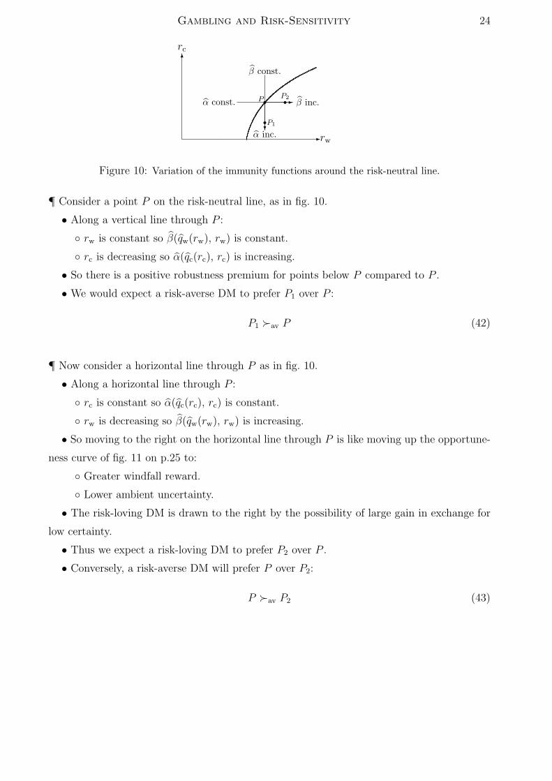
Figure 10: Variation of the immunity functions around the risk-neutral line.

¶ Consider a point P on the risk-neutral line, as in fig. 10.

• Along a vertical line through P :

◦ rw is constant so β(qw(rw), rw) is constant.

◦ rc is decreasing so α(qc(rc), rc) is increasing.

• So there is a positive robustness premium for points below P compared to P .

• We would expect a risk-averse DM to prefer P1 over P :

P1 ≻av P (42)

¶ Now consider a horizontal line through P as in fig. 10.

• Along a horizontal line through P :

◦ rc is constant so α(qc(rc), rc) is constant.◦ rw is decreasing so β(qw(rw), rw) is increasing.

• So moving to the right on the horizontal line through P is like moving up the opportune-

ness curve of fig. 11 on p.25 to:

◦ Greater windfall reward.

◦ Lower ambient uncertainty.

• The risk-loving DM is drawn to the right by the possibility of large gain in exchange for

low certainty.

• Thus we expect a risk-loving DM to prefer P2 over P .

• Conversely, a risk-averse DM will prefer P over P2:

P ≻av P2 (43)


6

-

Windfall Rewardrw

β(qw(rw), rw)

6

-

rc

rw

sssP

Q

R?

-

Figure 11: Optimal op-portuneness function ver-sus windfall reward.

Figure 12: Possible non-transitivity of preferences.

¶ We con summarize this discussion as follows, see fig. 12.

• For a risk-averse DM:

P ≻av R and R ≻av Q (44)

• However, we are not able to deduce the DM’s choice between P and Q. These points lie

on different robustness curves.

• We could explore the preference between P and Q by examining these different robustness

curves and the corresponding opportuneness curves.

• We cannot conclude that the DM has transitive preferences.

¶ In fact, non-transitive preferences are not rare.

• A very old example (Condorcet, 19th c.).

• Consider 3 options: A, B and C (e.g. apartments).

◦ Each option has 3 features: X, Y and Z, (e.g. location, size and price).

◦ The DM can rank each option according to each feature. E.g. table 1.

OptionsA B C

X low med highFeatures Y med high low

Z high low med

Table 1: Preference ranks of the options.

• If we compare options by voting on the features we see:

B ≻ A, C ≻ B, A ≻ C (45)

• The DM’s preferences among the options are non-transitive:

B ≻ A ≻ C ≻ B (46)


9 Pure Competition with Uncertain Cost

(Section 6.7)

¶ We will illustrate the risk-neutral line with a simple example.

¶ Production.

q = number of items to produce, which the DM must choose.

p(q) = known the sale price per item.

u(q) = uncertain cost of producing q items.

Assume all items are sold.

Profit is:

R(q) = qp(q)− u(q) (47)

¶ The info-gap model for uncertain manufacturing cost is:

U(α, u) = {u(q) : |u(q)− u(q)| ≤ αψ(q)} , α ≥ 0 (48)

u(q) and ψ(q) are known.

¶ The robustness and opportuneness functions for production volume q are:

α(q, rc) =qp(q)− rc − u(q)

ψ(q)(49)

β(q, rw) =rw − qp(q) + u(q)

ψ(q)(50)

¶ Special case:

ψ(q) = q and u(q) = u1q − u2qξ (51)

where 0 < ξ < 1, u1 > 0, u2 > 0 and u(q) > 0.u(q)q increases with q: diseconomy of scale:

d[u(q)/q]

dq= (1− ξ)u2q

ξ−2 > 0 (52)

Also:

p(q) = p0 = constant (53)

Pure competition: the firm’s production volume does not influence the market price.


¶ The immunity functions are:

α(q, rc) = p0 − u1 −rcq+ u2q

ξ−1 (54)

β(q, rw) = u1 − p0 +rwq

− u2qξ−1 (55)

¶ The robust-satisficing production volume is:

qc(rc) =

(rc

(1− ξ)u2

)1/ξ

(56)

which maximizes α(q, rc).

¶ The opportune-windfalling production volume, qw(rw), minimizes β(q, rw).

β(q, rw) cannot be negative, so qw(rw) is the solution for q of:

β(q, rw) = 0 (57)

or:

(p0 − u1)q + u2qξ = rw (58)

¶ The curve of risk-neutrality is the locus of points (rw, rc) at which:

qc(rc) = qw(rw) (59)

To formulate the risk-neutral line we substitute qc(rc) from eq.(56) for q in eq.(58) and

re-arrange to obtain:

rw = (p0 − u1)

(rc

(1− ξ)u2

)1/ξ

+rc

1− ξ(60)


¶ Fig. 13 shows risk-neutral lines for various ξ:

• ξ = ‘small’ =⇒ large dis-economy of scale.

• ξ = ‘large’ =⇒ small dis-economy of scale.

• Recall from fig. 12 on p.25:

P ≻av R and R ≻av Q (61)

• So, in fig. 13, risk-neutral lines shifts right with decreasing dis-economy of scale:

The DM becomes less risk-averse as the dis-economy of scale decreases.

-

6 ξ=0.01ξ=0.1 ξ=0.5

rcp0 − u1

rwp0 − u1

1

06310

Figure 13: Risk-neutral lines for various dis-economies of scale.

Lecture Notes on Gambling and Risk-Sensitivity

Documents