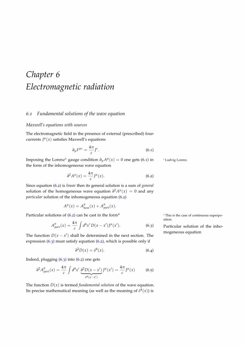
Chapter 6 Electromagnetic radiation 6.1 Fundamental solutions of the wave equation Maxwell’s equations with sources The electromagnetic field in the presence of external (prescribed) four- currents J μ ( x) satisfies Maxwell’s equations ∂ μ F μn = 4p c J n . (6.1) Imposing the Lorenz 1 gauge condition ∂ μ A μ ( x)= 0 one gets (6.1) in 1 Ludvig Lorenz. the form of the inhomogeneous wave equation ∂ 2 A μ ( x)= 4p c J μ ( x). (6.2) Since equation (6.2) is linear then its general solution is a sum of general solution of the homogeneous wave equation ∂ 2 A μ ( x)= 0 and any particular solution of the inhomogeneous equation (6.2) A μ ( x)= A μ hom ( x)+ A μ part ( x). Particular solutions of (6.2) can be cast in the form 2 2 This is the case of continuous superpo- sition. Particular solution of the inho- mogeneous equation A μ part ( x)= 4p c Z d 4 x 0 D( x - x 0 ) J μ ( x 0 ). (6.3) The function D( x - x 0 ) shall be determined in the next section. The expression (6.3) must satisfy equation (6.2), which is possible only if ∂ 2 D( x)= d 4 ( x). (6.4) Indeed, plugging (6.3) into (6.2) one gets ∂ 2 A μ part ( x)= 4p c Z d 4 x 0 ∂ 2 D( x - x 0 ) | {z } d 4 (x-x 0 ) J μ ( x 0 )= 4p c J μ ( x) (6.5) The function D( x) is termed fundamental solution of the wave equation. Its precise mathematical meaning (as well as the meaning of d 4 ( x)) is

Welcome message from author
This document is posted to help you gain knowledge. Please leave a comment to let me know what you think about it! Share it to your friends and learn new things together.
Transcript
Chapter 6Electromagnetic radiation
6.1 Fundamental solutions of the wave equation
Maxwell’s equations with sources
The electromagnetic field in the presence of external (prescribed) four-currents Jµ(x) satisfies Maxwell’s equations
∂µFµn =4p
cJn. (6.1)
Imposing the Lorenz1 gauge condition ∂µ Aµ(x) = 0 one gets (6.1) in 1 Ludvig Lorenz.
the form of the inhomogeneous wave equation
∂2 Aµ(x) =4p
cJµ(x). (6.2)
Since equation (6.2) is linear then its general solution is a sum of generalsolution of the homogeneous wave equation ∂2 Aµ(x) = 0 and anyparticular solution of the inhomogeneous equation (6.2)
Aµ(x) = Aµhom(x) + Aµ
part(x).
Particular solutions of (6.2) can be cast in the form2 2 This is the case of continuous superpo-sition.
Particular solution of the inho-mogeneous equation
Aµpart(x) =
4p
c
Zd4x0 D(x� x0)Jµ(x0). (6.3)
The function D(x � x0) shall be determined in the next section. Theexpression (6.3) must satisfy equation (6.2), which is possible only if
∂2D(x) = d4(x). (6.4)
Indeed, plugging (6.3) into (6.2) one gets
∂2 Aµpart(x) =
4p
c
Zd4x0 ∂2D(x� x0)| {z }
d4(x�x0)
Jµ(x0) =4p
cJµ(x) (6.5)
The function D(x) is termed fundamental solution of the wave equation.Its precise mathematical meaning (as well as the meaning of d4(x)) is
188 lecture notes on classical electrodynamics
given in the context of generalized functions (distributions). 3 In language 3 Distributions act on test functions as lin-ear functionals ( f , j) :=
Rdnx f (x)j(x).
Test functions are C•. They vanish at in-finity together with all their derivatives.
of distributions the fundamental solution for the d’Alembert operatorsatisfies the equation
(∂2D(x), j(x)) = (d4(x), j(x)) (6.6)
which means that the equality of ∂2D(x), j(x)) and (d4(x), j(x)) isrequired but not the equality of ∂2D(x) and d4(x). Thus, the solutionof the inhomogeneous wave equation has been reduced to the problemwhich does not depend on a particular form of four-current densityJµ. Note that the four-vector x0 can be omitted in the equation (6.6)because the differential operator ∂2 act on x.4 4 Alternatively, one can define new vari-
able z := x� x0.
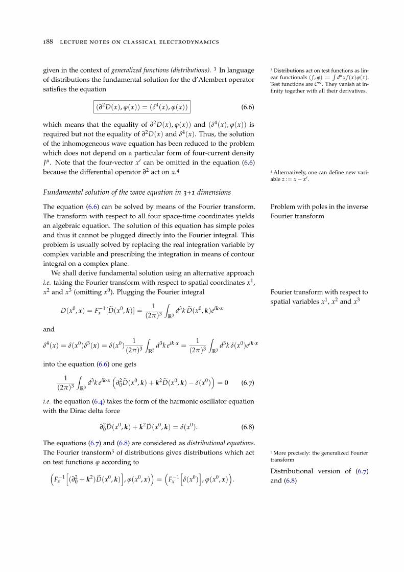
Fundamental solution of the wave equation in 3+1 dimensions
The equation (6.6) can be solved by means of the Fourier transform. Problem with poles in the inverseFourier transformThe transform with respect to all four space-time coordinates yields
an algebraic equation. The solution of this equation has simple polesand thus it cannot be plugged directly into the Fourier integral. Thisproblem is usually solved by replacing the real integration variable bycomplex variable and prescribing the integration in means of contourintegral on a complex plane.
We shall derive fundamental solution using an alternative approachi.e. taking the Fourier transform with respect to spatial coordinates x1,x2 and x3 (omitting x0). Plugging the Fourier integral Fourier transform with respect to
spatial variables x1, x2 and x3
D(x0, x) = F�1x [ eD(x0, k)] =
1(2p)3
Z
R3d3k eD(x0, k)eik·x
and
d4(x) = d(x0)d3(x) = d(x0)1
(2p)3
Z
R3d3k eik·x =
1(2p)3
Z
R3d3k d(x0)eik·x
into the equation (6.6) one gets
1(2p)3
Z
R3d3k eik·x
⇣∂2
0eD(x0, k) + k
2 eD(x0, k)� d(x0)⌘= 0 (6.7)
i.e. the equation (6.4) takes the form of the harmonic oscillator equationwith the Dirac delta force
∂20eD(x0, k) + k
2 eD(x0, k) = d(x0). (6.8)
The equations (6.7) and (6.8) are considered as distributional equations.The Fourier transform5 of distributions gives distributions which act 5 More precisely: the generalized Fourier
transformon test functions j according toDistributional version of (6.7)and (6.8)
⇣F�1
x
h(∂2
0 + k2) eD(x0, k)
i, j(x0, x)
⌘=⇣
F�1x
hd(x0)
i, j(x0, x)
⌘.
electromagnetic radiation 189
This equation can be cast in the form⇣(∂2
0 + k2) eD(x0, k), ej(x0, k)
⌘=⇣
d(x0), ej(x0, k)⌘
, (6.9)
where ej(x0, k) ⌘ F�1x [j](x0, k)) is a test function. The equation (6.9) is
a distributional version of (6.8).The solution of (6.8) is called fundamental solution of the harmonic
oscillator and it reads The fundamental solution of har-monic oscillator equation
eDret/adv(x0, k) = ±q(±x0)sin(kx0)
k, (6.10)
where k = |k|. eDret and eDadv are, respectively, retarded (upper sign) andadvanced (bottom sign) solutions.
We shall show that eDret is the solution in distributional sense. De-noting for convenience x ⌘ x0 and Z(x) ⌘ sin(kx)
k and using definitionof generalized derivative of distributions Generalized derivative of a dis-
tribution( f (n)(x), j(x)) := (�1)n( f (x), j(n)(x))
one gets Proof for the retarded function
( eD00 + k2 eD, j) = ( eD, j00) + (k2 eD, j) =
=Z •
�•dx q(x)Z(x)j00(x) +
Z •
�•dx q(x)k2Z(x)j(x)
=Z •
0dx Z(x)j00(x) +
Z •
0dx k2Z(x)j(x) = · · ·
Integration by parts gives
· · · = Z(x)j0(x)���•
0�
Z •
0dxZ0(x)j0(x) +
Z •
0dx k2Z(x)j(x) =
= Z(x)j0(x)���•
0� Z0(x)j(x)
���•
0+Z •
0dx (Z00(x) + k2Z(x))| {z }
0
j(x).
Since test functions and all their derivatives vanish at infinity j(•) ⌘ 0,j(n)(•) ⌘ 0 and Z(0) = 0 and Z0(0) = 1 then
( eD00 + k2 eD, j) = j(0) = (d(x), j(x)), (6.11)
where the second equality reflects the definition of the d�distribution.The proof for the advanced function is almost identical. In such a case (d(x), j(x)) := j(0)
Proof for the advanced functionwe take eD(x) = �q(�x)Z(x) which gives
( eD00 + k2 eD, j) =�Z 0
�•dx Z(x)j00(x)�
Z 0
�•dx k2Z(x)j(x)
=� Z(x)j0(x)���0
�•+ Z0(x)j(x)
���0
�•�
�
Z 0
�•dx (Z00(x) + k2Z(x))| {z }
0
j(x)
= j(0) = (d(x), j(x)).
190 lecture notes on classical electrodynamics
For explicitly given the function eDret/adv(x0, k) one gets solutions of The inverse Fourier transform ofeDret/adv(x0, k)(6.6) as the inverse Fourier transform
Dret/adv(x0, x) =1
(2p)3
Zd3k eik·x eDret/adv(x0, k)
=±q(±x0)(2p)3
Zd3k eik·x sin(kx0)
k.
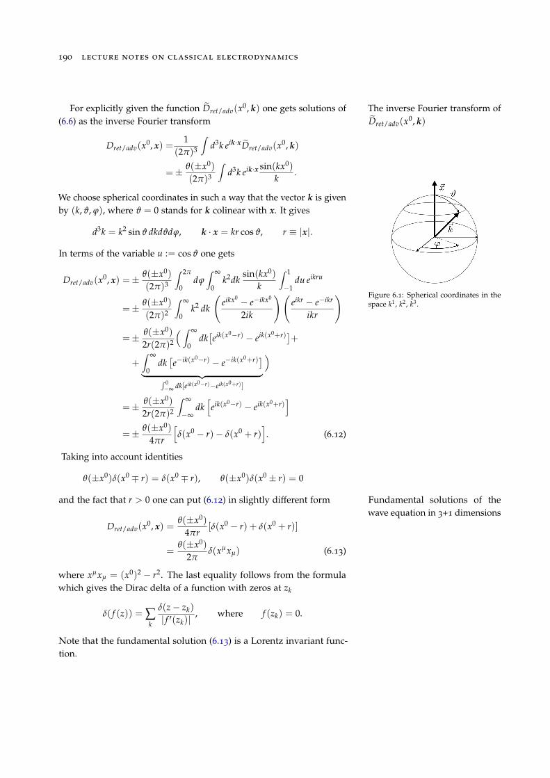
We choose spherical coordinates in such a way that the vector k is givenby (k, J, j), where J = 0 stands for k colinear with x. It gives
d3k = k2 sin J dkdJdj, k · x = kr cos J, r ⌘ |x|.
Figure 6.1: Spherical coordinates in thespace k1, k2, k3.
In terms of the variable u := cos J one gets
Dret/adv(x0, x) =±q(±x0)(2p)3
Z 2p
0djZ •
0k2dk
sin(kx0)k
Z 1
�1du eikru
=±q(±x0)(2p)2
Z •
0k2 dk
eikx0� e�ikx0
2ik
! eikr � e�ikr
ikr
!
=±q(±x0)2r(2p)2
⇣ Z •
0dk⇥eik(x0�r)
� eik(x0+r)⇤+
+Z •
0dk⇥e�ik(x0�r)
� e�ik(x0+r)⇤
| {z }R 0�• dk[eik(x0�r)�eik(x0+r)]
⌘
=±q(±x0)2r(2p)2
Z •
�•dkheik(x0�r)
� eik(x0+r)i
=±q(±x0)
4pr
hd(x0
� r)� d(x0 + r)i. (6.12)
Taking into account identities
q(±x0)d(x0⌥ r) = d(x0
⌥ r), q(±x0)d(x0± r) = 0
and the fact that r > 0 one can put (6.12) in slightly different form Fundamental solutions of thewave equation in 3+1 dimensions
Dret/adv(x0, x) =q(±x0)
4pr[d(x0
� r) + d(x0 + r)]
=q(±x0)
2pd(xµxµ) (6.13)
where xµxµ = (x0)2 � r2. The last equality follows from the formulawhich gives the Dirac delta of a function with zeros at zk
d( f (z)) = Âk
d(z� zk)| f 0(zk)|
, where f (zk) = 0.
Note that the fundamental solution (6.13) is a Lorentz invariant func-tion.
electromagnetic radiation 191
Fundamental solution of the wave equation without explicit dependenceon one or two variables
When a physical system possesses certain symmetries i.e. their solu- Physical systems without depen-dence on x3 coordinatetions do not depend on one or more coordinates, then a part of the
d’Alembert operator associated with these variables became irrelevant.For instance, ∂2y(x0, x1, x2) in 3+1 dimensions reads
(∂20 � ∂2
1 � ∂22 � ∂2
3)y(x0, x1, x2) = (∂20 � ∂2
1 � ∂22)y(x0, x1, x2).
Such systems behave effectively as some lower-dimensional systems.The independence of physical fields on certain number of coordinates
can be expressed in the formalism of generalized functions assumingthat test functions do not depend on these coordinates. Effectively, onehas to replace
j(x0, x1, x2, x3)! j(x0, x1, x2).
This assumption allows us to obtain low-dimensional fundamentalsolutions integrating over irrelevant coordinates.
We shall consider a class of test functions that are constant in direc- Reduction D(3) ! D(2)
tion given by coordinate x3. The generalized function (∂20 � ∂2
1 � ∂22 �
∂23)D(3)
ret (x) acts on any test function j(x) as a linear functional in 3+1dimensions i.e. it associates a real number with j . This number isobtained by integration over all (four) spacetime variables
⇣(3+1)
∂2 D(3)ret (x), j(x)
⌘=⇣
D(3)ret (x0, x),
(2+1)
∂2 j�
0z}|{∂2
3 j⌘
=Z
R3dx0dx1dx2
h Z •
�•dx3D(3)
ret (x0, x)i(2+1)
∂2 j
(6.14)
where the independence of j on x3 allows us to integrate out D(3)ret (x)
(2+1)∂2 := ∂2
0 � ∂21 � ∂2
2over x3
D(2)ret (x0, x1, x2) :=
Z •
�•dx3D(3)
ret (x0, x1, x2, x3). (6.15)
The right hand side of (6.14) can be cast in the form
⇣D(2)
ret ,(2+1)
∂2 j(x0, x1, x2)⌘=⇣(2+1)
∂2 D(2)ret , j(x0, x1, x2)
⌘, (6.16)
where ( f , j) is a three-dimensional integral
( f , j) =Z
R3dx0dx1dx2 f j.
Since the test function j does not depend on the x3 variable then thed�distribution acts on it in the following way⇣
d4(x), j(x0, x1, x2)⌘= j(0, 0, 0) =
⇣d(x0)d(x1)d(x2), j(x0, x1, x2)
⌘.
192 lecture notes on classical electrodynamics
One can conclude that D(2)ret obeys the following distributional equation
⇣(2+1)
∂2 D(2)ret (x), j(x)
⌘= (d3(x), j(x)), (6.17)
where x = (x0, x1, x2). Thus D(2)ret has meaning of fundamental solution
of the wave equation in 2 + 1 dimensions.In order to get a fundamental solution for the d’Alembert operator Reduction D(2) ! D(1)
in 1 + 1 dimensions one has to take a class of test functions whichonly depends on x0 and x1. Expression (D(2)
ret , j) contains integral overx2, however, j does not depend on this variable. Hence D(2)
ret can beexplicitly integrated out on the variable x2
D(1)ret (x0, x1) :=
Z •
�•dx2D(2)(x0, x1, x2). (6.18)
where x = (x0, x1). In the next two section we shall derive an explicitform of the solutions D(2)
ret and D(1)ret .
Fundamental solution in 2 + 1 dimensions
In this section we shall obtain the explicit form of the generalizedfunction D(2)
ret . In order to simplify the notation we define y := (x1, x2)
and y := |y|. We consider the integral over R4 of the product offunctions D(3)
ret (x) and j(x0, x1, x2) 6 6 It is more convenient to study a four-dimensional integral than the integral ofD(3)
ret over the variable x3 alone.⇣
D(3)ret (x), j(x0, y)
⌘
(3+1)=
=Z •
�•dx0
Z
R2d2y j(x0, y)
Z •
�•dx3 q(x0)
4p|x|d(x0
� |x|)
=Z •
0dx0
Z
R2d2y j(x0, y)
Z •
�•dx3 1
4p
d(x0 �p
y2 + (x3)2)py2 + (x3)2
= . . .
The d�function depends on the x3 variable through the function
f (x3) := x0�
qy2 + (x3)2
and thus it can be cast in the form
d( f (x3)) = Âk
d(x3 � x3k)
| f 0(x3)|x3=x3k
,
where solutions of the equation f (x3k) = 0 are denoted by x3
k . There aretwo such solutions
x31 = �
q(x0)2 � y2, x3
2 = +q(x0)2 � y2.
They are real-valued expressions for |y| x0, then Restriction |y| x0
electromagnetic radiation 193
d( f (x3)) =d(x3 � x3
1)�����x3
1py2+(x3
1)2
����+
d(x3 � x32)�����
x32p
y2+(x32)
2
����
=x0
p(x0)2 � y2
hd(x3
� x31) + d(x3
� x32)i
.
The condition |y| x0 restricts the integration region to the interior ofa disc with radius y = x0. One gets
. . . =Z •
0dx0
Z
|y|x0d2y j(x0, y)⇥
⇥
Z •
�•dx3 1
4p
x0p
(x0)2�y2
⇥d(x3 � x3
1) + d(x3 � x32)⇤
py2 + (x3)2
=
=Z •
0dx0
Z
|y|x0d2y j(x0, y)
14p
x0p(x0)2 � y2
2x0 = . . .
Including the Heaviside’s function q(x0 � |y|) one can extend the inte-gration area to the space R⇥R2, thus
. . . =Z •
�•dx0
Z
R2d2y j(x0, y)
12p
q(x0 � |y|)p(x0)2 � |y|2
.
The (2+1) dimensional fundamental solution D(2)ret is of the form The fundamental (retarded) solu-
tion for the d’Alembert operatorin 2+1 dimensionsD(2)
ret (x) =1
2p
q(x0 � |x|)p(x0)2 � |x|2
, (6.19)
where we the argument x in D(2)(x) means x = (x0, x), where x ⌘
(x1, x2).
Fundamental solution in 1 + 1 dimensions
Let us take the expression
(D(2)ret , j)(2+1) =
Z •
�•dx0
Z •
�•dx1
Z •
�•dx2D(2)(x0, x1, x2)
�j(x0, x1)
=Z •
�•dx0
Z •
�•dx1
"Z •
�•dx2 1
2p
q(x0 � |x|)p(x0)2 � |x|2
#j(x0, x1)
= . . .
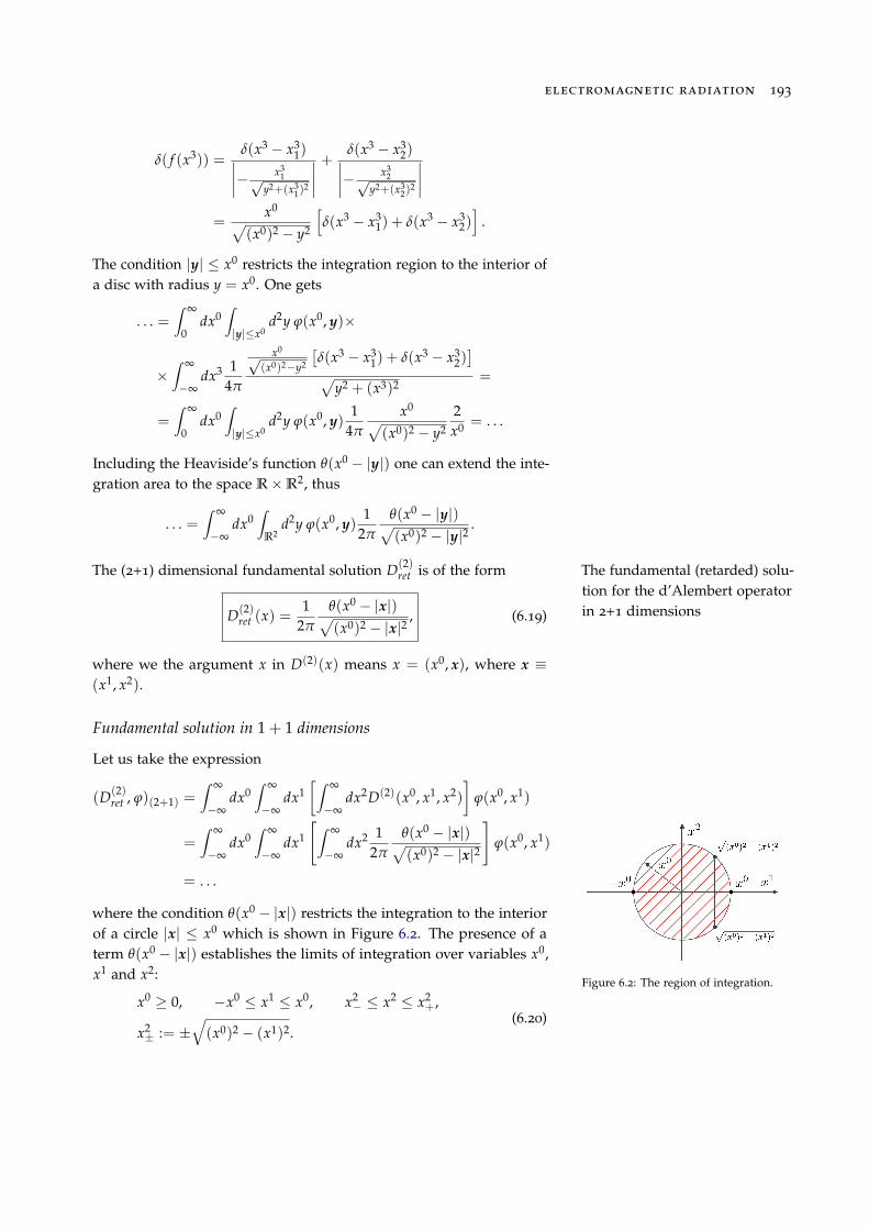
Figure 6.2: The region of integration.
where the condition q(x0 � |x|) restricts the integration to the interiorof a circle |x| x0 which is shown in Figure 6.2. The presence of aterm q(x0 � |x|) establishes the limits of integration over variables x0,x1 and x2:
x0� 0, �x0
x1 x0, x2
� x2 x2
+,
x2± := ±
q(x0)2 � (x1)2.
(6.20)
194 lecture notes on classical electrodynamics
It gives
. . . =Z •
0dx0
Z x0
�x0dx1
"Z x2+
x2�
dx2 12p
1p(x0)2 � (x1)2 � (x2)2
#j(x0, x1)
=1
2p
Z •
0dx0
Z x0
�x0dx1
"2Z x2
+
0
dx2p(x0)2 � (x1)2
1r1� (x2)2
(x0)2�(x1)2
#⇥
⇥ j(x0, x1) = . . .
In terms of new variable
u :=x2
p(x0)2 � (x1)2
, du =dx2
p(x0)2 � (x1)2
the last expression takes the form
. . . =1p
Z •
0dx0
Z x0
�x0dx1h Z 1
0
dup
1� u2| {z }
arcsin(1)�arcsin(0)= p2
ij(x0, x1)
=12
Z •
0dx0
Z x0
�x0dx1 j(x0, x1)
=Z •
�•dx0
Z •
�•dx1
12
q(x0� |x1
|)
�j(x0, x1).
Thus, the fundamental solution of the wave equation in 1 + 1 dimen-sions is of the form Fundamental solution of the
wave equation in 1 + 1 dimen-sionsD(1)
ret (x) =12
q⇣
x0� |x1
|
⌘. (6.21)
Huygen’s principle
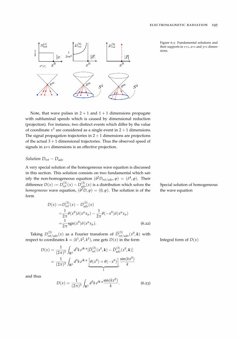
Comparing the fundamental solutions (6.13), (6.19) and (6.21), respec-tively, in 3+1, 2+1 and 1+1 dimensions one can conclude that in lowerdimensions the solutions depend on functions of variables |x| x0.The point is that these functions are different from the d� like gener-alize function (6.13). For this reason the solution of wave equation atany point (x0, x) depends on initial data in certain region of spacetime.Due to causality, such regions are localized inside the past light cone ofthe event (x0, x) considered as the light-cone apex.
On the contrary, the solutions in 3+1 dimensions depend exclusivelyon events that are causally related with (x0, x) i.e. they belong to theconical surface of the light-cone. It means that solutions of the waveequation in 3+1 dimensions propagate with the speed of light. This fact isknown as Huygen’s principle. In fact, the Huygen’s principle is also truein higher n + 1 dimensions where n = 3, 5, 7, . . ..
electromagnetic radiation 195
Figure 6.3: Fundamental solutions andtheir supports in 1+1, 2+1 and 3+1 dimen-sions.
Note, that wave pulses in 2 + 1 and 1 + 1 dimensions propagatewith subluminal speeds which is caused by dimensional reduction(projection). For instance, two distinct events which differ by the valueof coordinate x3 are considered as a single event in 2 + 1 dimensions.The signal propagation trajectories in 2 + 1 dimensions are projectionsof the actual 3 + 1 dimensional trajectories. Thus the observed speed ofsignals in 2+1 dimensions is an effective projection.
Solution Dret � Dadv
A very special solution of the homogeneous wave equation is discussedin this section. This solution consists on two fundamental which sat-isfy the non-homogeneous equation (∂2Dret/adv, j) = (d4, j). Theirdifference D(x) := D(3)
ret (x)� D(3)adv(x) is a distribution which solves the Special solution of homogeneous
the wave equationhomogeneous wave equation, (∂2D, j) = (0, j). The solution is of theform
D(x) :=D(3)ret (x)� D(3)
adv(x)
=1
2pq(x0)d(xµxµ)�
12p
q(�x0)d(xµxµ)
=1
2psgn(x0)d(xµxµ). (6.22)
Taking D(3)ret/adv(x) as a Fourier transform of eD(3)
ret/adv(x0, k) withrespect to coordinates k = (k1, k2, k3), one gets D(x) in the form Integral form of D(x)
D(x) =1
(2p)3
Z
R3d3k eik·x[ eD(3)
ret (x0, k)� eD(3)adv(x0, k)]
=1
(2p)3
Z
R3d3k eik·x
hq(x0) + q(�x0)
i
| {z }1
sin(kx0)k
and thus
D(x) =1
(2p)3
Z
R3d3k eik·x sin(kx0)
k. (6.23)
196 lecture notes on classical electrodynamics
Other solution of the homogeneous wave equation can be obtainedtaking the derivative of D(x) with respect to spatial coordinate x0. Itgives
D1(x) :=∂D(x)
∂x0 =1
(2p)3
Z
R3d3k eik·x cos(kx0). (6.24)
Solutions (6.23) and (6.24) have the following properties
D(0, x) = 0, D1(0, x) = d3(x),∂D1∂x0 (x0, x)
����x0=0
= 0. (6.25)
Functions D(x0, x) and D1(x0, x) form two linearly independent solutionsof the wave equation. Moreover, taking into account properties (6.25) onecan get the formula for a solution of the wave equation which satisfiesthe initial data. We shall discuss this subject in the next section.
6.2 Boundary problems
Any general solution Aµ of the equation ∂2 Aµ = 4pc Jµ can be altered
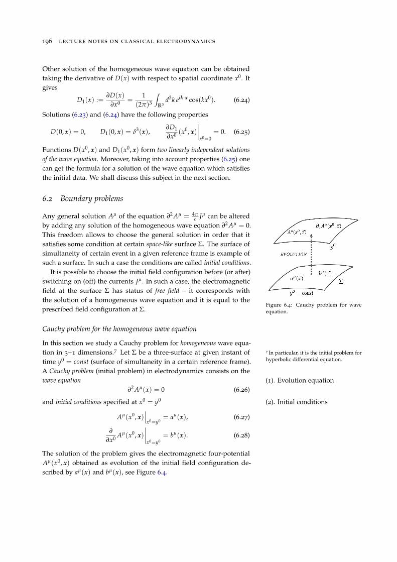
by adding any solution of the homogeneous wave equation ∂2 Aµ = 0.This freedom allows to choose the general solution in order that itsatisfies some condition at certain space-like surface S. The surface ofsimultaneity of certain event in a given reference frame is example ofsuch a surface. In such a case the conditions are called initial conditions.
Figure 6.4: Cauchy problem for waveequation.
It is possible to choose the initial field configuration before (or after)switching on (off) the currents Jµ. In such a case, the electromagneticfield at the surface S has status of free field – it corresponds withthe solution of a homogeneous wave equation and it is equal to theprescribed field configuration at S.
Cauchy problem for the homogeneous wave equation
In this section we study a Cauchy problem for homogeneous wave equa-tion in 3+1 dimensions.7 Let S be a three-surface at given instant of 7 In particular, it is the initial problem for
hyperbolic differential equation.time y0 = const (surface of simultaneity in a certain reference frame).A Cauchy problem (initial problem) in electrodynamics consists on thewave equation (1). Evolution equation
∂2 Aµ(x) = 0 (6.26)
and initial conditions specified at x0 = y0 (2). Initial conditions
Aµ(x0, x)���x0=y0
= aµ(x), (6.27)
∂
∂x0 Aµ(x0, x)
����x0=y0
= bµ(x). (6.28)
The solution of the problem gives the electromagnetic four-potentialAµ(x0, x) obtained as evolution of the initial field configuration de-scribed by aµ(x) and bµ(x), see Figure 6.4.
electromagnetic radiation 197
By means of Fourier transform we map the Cauchy problem in-volving partial differential equation by an initial problem for ordinarydifferential equation. This requires transform acting on spatial variablesx. Plugging the four-potential represented by integrals
Aµ(x0, x) = F�1[ eAµ(x0, k)] =1
(2p)3
Z
R3d3keik·x eAµ(x0, k) (6.29)
into the wave equation (6.26) one gets The harmonic oscillator equation
(∂20 + k
2) eAµ(x0, k) = 0. (6.30)
The harmonic oscillator equation (6.30) depends on a single variable x0.The variable k has the status of free parameter. Applying the Fouriertransform, the initial conditions yield Fourier transform of the initial
conditionseaµ(k) := F[aµ(x)] = eAµ(x0, k)
���x0=y0
, (6.31)
ebµ(k) := F[bµ(x)] =∂ eAµ
∂x0 (x0, k)
�����x0=y0
. (6.32)
To solve (6.30) we choose two linearly independent solutions of theequation
(∂20 + k2) eD(z0, k) = 0
where the variable x0 has been substituted by z0 := x0� y0 and k := |k|.They have the form Linearly independent solutions
of harmonic oscillatoreD(z0, k) =
sin(kz0)k
, eD1(z0, k) =∂ eD∂x0 (z
0, k) = cos(kz0)
and satisfy conditions
eD(0, k) = 0, eD1(0, k) = 1.
A general solution of (6.30) is given by linear combination of eD and eD1
eAµ(x0, k) = aµ eD1(x0� y0, k) + bµ eD(x0
� y0, k), (6.33)
where aµ and bµ are two constant four-vectors. Imposing the initialconditions (6.31) and (6.32) on (6.33) one gets
aµ = aµ(k), bµ = bµ(k).
Thus, the solution of (6.30) reads Solution of transformed equation
eAµ(x0, k) = eaµ(k) eD1(x0� y0, k) + ebµ(k) eD(x0
� y0, k). (6.34)
The solution of the Cauchy problem is given by the inverse Fourier Solution of partial differentialequation:
eAµ(x0, k)! Aµ(x0, x)
transform of eAµ(x0, k) which solves (6.34). Plugging (6.34) into (6.29)where coefficients are represented in the form
eaµ(k) = F[aµ(y)] =Z
d3ye�ik·yaµ(y),
ebµ(k) = F[bµ(y)] =Z
d3ye�ik·ybµ(y),
198 lecture notes on classical electrodynamics
and similarly
eD(x0� y0, k) = F[D(x0
� y0, z)] =Z
d3ze�ik·zD(x0� y0, z)
eD1(x0� y0, k) = F[D1(x0
� y0, z)] =Z
d3ze�ik·zD1(x0� y0, z)
one gets
Aµ(x0, x) =1
(2p)3
Zd3keik·x eAµ(x0, k) =
=1
(2p)3
Zd3keik·x
Zd3ye�ik·y
Zd3ze�ik·z
⇥
⇥
haµ(y)D1(x0
� y0, z) + bµ(y)D(x0� y0, z)
i. (6.35)
This expression can be simplified using integral representation for theDirac delta distribution
1(2p)3
Zd3keik·(x�y�z) = d3(x� y� z).
Integrating over variables z1, z2 and z3 one gets Solution of the wave equationthat satisfy the initial conditions
Aµ(x0, x) =Z
Sd3y
haµ(y)D1(x0
� y0, x� y) + bµ(y)D(x0� y0, x� y)
i
(6.36)where the integral is taken over the hypersurface of initial conditions aty0 = const.
We shall express this formula in the alternative form. First, one cansee thet D(z) is an anti-symmetric function of zµ. This can be seenexplicitly from
D(�z0,�z) =1
(2p)3
Zd3ke�ik·z sin(|k|(�z0))
|k|= �D(z0, z), (6.37)
where in the last step absorb the sign on definition of new variable ofintegration k! �k
Z •
�•dki . . .!
Z�•
+•(�dki) . . . =
Z •
�•dki . . .
Second, the function D1(x� x0), defined as derivative of D(x� x0) withrespect to x0, can be represented alternatively as derivative with respectto x00. Thus we have
D1(x� x0) =∂
∂x0 D(x0� x00, x� x
0) = �∂
∂x00D(x0
� x00, x� x0)
=∂
∂x00D(x00 � x0, x
0� x) =
∂
∂x00D(x0 � x).
The function D1 for x0 = y ⌘ (y0, y) i.e. D1(x0 � y0, x� y) ⌘ D1(x� y)can be cast in the form
D1(x� x0)���x0=y
=∂
∂x00D(x0 � x)
���x0=y
. (6.38)
electromagnetic radiation 199
Similarly, the function D(x� y) reads
D(x� y) = D(x� x0)���x0=y
= �D(x0 � x)���x0=y
. (6.39)
Finally, the functions aµ(y) and bµ(y) can be cast in the form
aµ(y) = Aµ(x0)���x0=y
, bµ(y) =∂Aµ
∂x00(x0)
���x0=y
. (6.40)
Plugging (6.38), (6.39) and (6.40) into (6.36) one gets8 8 Aµ and its derivative at x0 = y on theright hand side of expression (6.41) areprescribed (a priori given) functions.
Aµ(x) =Z
S(y)d3x0
Aµ(x0)
∂D(x0 � x)∂x00
�∂Aµ(x0)
∂x00D(x0 � x)
�(6.41)
where the four-vectors x0 give events on S(y).It can be checked that (6.41) solves the Cauchy problem. Acting with Verification of formula (6.41):
∂2 on both sides of (6.41) one gets that Aµ(x) given by (6.41) satisfiesthe wave equation
∂2 Aµ(x) =Z
S(y)d3x0
hAµ(x0)
∂
∂x00∂2D(x0 � x)| {z }
0
�∂Aµ(x0)
∂x00∂2D(x0 � x)| {z }
0
i= 0
where D(x0 � x) is a solution of the homogeneous wave equation (1). It satisfies the evolution equa-tionaccording to
∂2D(x0 � x) =1
(2p)3
Zd3k
h∂2
0 �r2i
eik·(x0�x) sin(|k|(x00 � x0))
|k|
=1
(2p)3
Zd3kh� |k|
2 + k2ieik·(x
0�x) sin(|k|(x00 � x0))|k|
= 0.
The initial conditions at hypersurface x 2 S(y) i.e. x0 = x00 = y0 aresatisfied. It can be seen from
D(x0 � x)���x2S(y)
=1
(2p)3
Zd3k eik·(x
0�x) sin(|k|(y0 � x0))|k|
����x0=y0
=
= 0,
∂D(x0 � x)∂x00
���x2S(y)
=1
(2p)3
Zd3keik·(x
0�x) cos(|k|(y0� x0))
����x0=y0
=
= d3(x0� x),
∂D(x0 � x)∂x0
���x2S(y)
= �d3(x0� x),
∂2D(x0 � x)∂x0∂x00
���x2S(y)
=1
(2p)3
Zd3keik·(x
0�x)|k| sin(|k|(y0
� x0))
����x0=y0
=
= 0.
200 lecture notes on classical electrodynamics
Thus (6.41) at x0 = y0 and with the above formulas yelds (2). It satisfies the initial condi-tions
Aµ(x)���x0=y0
=Z
S(y)d3x0 Aµ(y0, x
0) d3(x0� x) = Aµ(y0, x) = aµ(x).
A derivative of (6.41) w.r.t. x0 at x0 = y0 reads
∂Aµ(x)∂x0
����x0=y0
=Z
S(y)d3x0
∂Aµ
∂x00d3(x
0� x) =
∂Aµ
∂x00(x00, x)
����x00=y0
= bµ(x).
The initial condition can be generalized by substitution of the surface Generalization Cauchy problemto arbitrary Cauchy surfaceof simultaneity a generic space-like surface.
A Cauchy surface S(y) is a space-like three surface9 which is inter- 9 Locally it looks like a piece of the sur-face of simultaneity in a certain inertialreference frame.
sected by every time-like curve (e.g worldline) exactly once. The intervalassociated with two events belonging to the Cauchy surface is negative,Ds2 < 0.
When the hyperplane x0 = y0 is replaced by the Cauchy surfaceS then (6.41) must be modified in the wave that it contains Lorentzinvariant (or covariant) expressions.
• The volume element d3x0 = d3S0 is replaced by
d3S0 ! d3Sn =13!p�genabg
∂(xaxbxg)
∂(t1t2t3)dt1dt2dt3.
• The derivative of the electromagnetic four-potential with respect tox00 is replaced by
∂Aµ
∂x00!
∂Aµ
∂x0n.
• The expression ∂D(x0�x)∂x00
���x0=x00
= d3(x0 � x) requires substitution of
the Dirac delta distribution by the following one
d3(x0� x)! nnd3(x
0� x) ⌘ d3
µ(x0� x)
where nn = nn(x0) is a time-like four-vector, n2 = 1, orthogonalto the surface S i.e nndx0n = 0. The spatial three-volume elementd3Sn(x0)nn(x0) is equal to d3S00(x0) in a local rest frame S0 at x0 inwhich n0n = dn
0 .
Thus
∂D(x0 � x)∂x00
����x0=x00=y0
!∂D(x0 � x)
∂x0n
����x2S
= nnd3(x0� x).
Finally, we get the generalization of (6.41) in the form Solution of the Cauchy problemthat satisfies initial conditions atthe Cauchy surface SAµ(x) =
Z
S(y)d3Sn(x0)
Aµ(x0)
∂
∂x0nD(x0 � x)� D(x0 � x)
∂Aµ
∂x0n(x0)
�
(6.42)
electromagnetic radiation 201
where Aµ(x0) and ∂Aµ
∂x0n (x0) are prescribed functions. They give the elec-tromagnetic field at S(y)
Aµ(x0)���x02S(y)
⌘ aµ(y),∂Aµ
∂x0n(x0)
�����x02S(y)
⌘ bµ(y).
Indeed, for x 2 S(y) the solution (6.42) reads
Aµ(x)���x2S(y)
=Z
S(y)d3Sn(x0)
hAµ(x0)nnd3(x
0� x)� 0
i= aµ(y).
Similarly, taking derivative with respect to x0 and evaluating the result-ing expression at the Cauchy surface S one gets
∂Aµ(x)∂x0
���x2S(y)
=Z
Sd3Sn(x0)
"0�
�d3(x0�x)z }| {
∂D∂x0 (x0 � x)
���x2S(y)
∂Aµ
∂x0n(x0)
#= bµ(y).
Independence of the solutionon the choice of the Cauchy sur-face
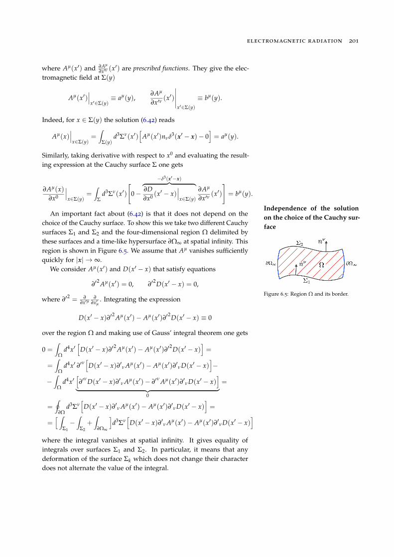
Figure 6.5: Region W and its border.
An important fact about (6.42) is that it does not depend on thechoice of the Cauchy surface. To show this we take two different Cauchysurfaces S1 and S2 and the four-dimensional region W delimited bythese surfaces and a time-like hypersurface ∂W• at spatial infinity. Thisregion is shown in Figure 6.5. We assume that Aµ vanishes sufficientlyquickly for |x|! •.
We consider Aµ(x0) and D(x0 � x) that satisfy equations
∂02 Aµ(x0) = 0, ∂0
2D(x0 � x) = 0,
where ∂02 = ∂∂x0µ
∂∂x0µ
. Integrating the expression
D(x0 � x)∂02 Aµ(x0)� Aµ(x0)∂02D(x0 � x) ⌘ 0
over the region W and making use of Gauss’ integral theorem one gets
0 =Z
Wd4x0
hD(x0 � x)∂02 Aµ(x0)� Aµ(x0)∂02D(x0 � x)
i=
=Z
Wd4x0 ∂0n
hD(x0 � x)∂0n Aµ(x0)� Aµ(x0)∂0nD(x0 � x)
i�
�
Z
Wd4x0
h∂0
nD(x0 � x)∂0n Aµ(x0)� ∂0n Aµ(x0)∂0nD(x0 � x)
i
| {z }0
=
=I
∂Wd3Sn
hD(x0 � x)∂0n Aµ(x0)� Aµ(x0)∂0nD(x0 � x)
i=
=h Z
S1�
Z
S2+Z
∂W•
id3Sn
hD(x0 � x)∂0n Aµ(x0)� Aµ(x0)∂0nD(x0 � x)
i
where the integral vanishes at spatial infinity. It gives equality ofintegrals over surfaces S1 and S2. In particular, it means that anydeformation of the surface Sk which does not change their characterdoes not alternate the value of the integral.
202 lecture notes on classical electrodynamics
If the the space-like surface S contains x then any event x0 at S isconnected with x by a space-like four-vector. It leads to vanishing ofD(x0 � x) and gives
Aµ(x) =Z
S(y)d3Sn(x0) Aµ(x0)
∂
∂x0nD(x0 � x).
The solution is also unique. Let Aµ1 (x) and Aµ
2 (x) be two solutions ofthe equation ∂2 Aµ(x) = 4p
c Jµ(x) that satisfy simultaneously the initial The uniqueness of solution ofthe Cauchy problemconditions
Aµ1 (x)
���S(y)
= Aµ2 (x)
���S(y)
= aµ(y) (6.43)
and∂0 Aµ
1 (x)���S(y)
= ∂0 Aµ2 (x)
���S(y)
= bµ(y). (6.44)
The function Aµ0 (x) := Aµ
1 (x)� Aµ2 (x) is a solution of homogeneous
d’Alembert equation ∂2 Aµ0 (x) = 0 and satisfies initial conditions
Aµ0 (x)
���S(y)
= 0, ∂0 Aµ0 (x)
���S(y)
= 0. (6.45)
It follows from (6.42) that the only solution of the homogeneous waveequation, which satisfies (6.42), is a constant solution Aµ
0 (x) = 0.We conclude that Aµ
1 (x) = Aµ2 (x) i.e. the solution of the inhomo-
geneous equation that satisfies initial conditions Aµ(x)���S(y)
= aµ(y)
and ∂0 Aµ(x)���S(y)
= bµ(y) is unique.
Retarded and advanced solutions
The Cauchy problem is well-possed if
1. a solution exists,
2. the solution is unique,
3. the solution’s behaviour changes continuously with the initial condi-tions.
The initial field configuration is prescribed at the space-like surfaceS(y). In particular, this configuration can be chosen at the simultaneitysurface, x0 = y0. The field configurations at S(y) are frequently de-termined in the remote past or in the remote future i.e. before (after)switching on (off) the external sources. Thus we shall consider
Jµ(x)|x2S(y) ⌘ 0.
It means that the initial (final) field configuration is a free electromag-netic field which solves the homogeneous wave equation. The solution
electromagnetic radiation 203
defined in the remote past is denoted by Aµin(x) wheres the solution
defined in the remote future is denoted by Aµout(x). The retarded and
advanced potentials read Retarded and advanced poten-tials
Aµret(x) :=
4p
c
Zd4x0Dret(x� x0)Jµ(x0), (6.46)
Aµadv(x) :=
4p
c
Zd4x0Dadv(x� x0)Jµ(x0). (6.47)
They solve the inhomogeneous wave equation, namely
∂2 Aµretadv
(x) =4p
c
Zd4x0d4(x� x0)Jµ(x0) =
4p
cJµ(x).
One can construct general solutions by inclusion of incoming or outgo-ing free fields
Aµ(x) = Aµin(x) + Aµ
ret(x), (6.48)
Aµ(x) = Aµout(x) + Aµ
adv(x). (6.49)
Potentials (6.48) and (6.49) represent the same field at x, thus
Aµin(x) + Aµ
ret(x) = Aµout(x) + Aµ
adv(x). (6.50)
The field Aµret(x) describes emission of the field by sources Jµ whereas
Aµadv(x) describes a field absorption.The expression (6.48) is a solution of the inhomogeneous wave equa-
tion with the initial configuration which is a free electromagnetic fieldin the remote past x0 ! �•. Similarly, expression (6.49) gives the solu-tion of the inhomogeneous wave equation for the final configurationbeing free electromagnetic field in the remote future x0 ! +•. The Lorenz condition
Considering that the fields Aµin(x) and Aµ
out(x) satisfy the Lorenzcondition Free fields which (by assump-
tion) satisfy the Lorenz condition∂µ Aµin(x) = 0, ∂µ Aµ
out(x) = 0, (6.51)
one concludes that (6.48) and (6.49) satisfy this condition as well. Toprove this statement we choose a region W. Its border consists of twospace-like three-surfaces S1 and S2 and a time-like three-surface atspatial infinity S•,
∂W = S1 [ S2 [ S•.
We assume that the four-currents vanish outside a certain compactregion E3. It means that Four-currents (by assumption)
vanish at S•Jµ��S•⌘ 0. (6.52)
They are called localized currents. taking four-divergence of solutions
204 lecture notes on classical electrodynamics
(6.48) and (6.49) one gets
∂Aµ
∂xµ (x) =
0z }| {∂
∂xµ Aµin
out(x) +
4p
c
Z
Wd4x0
∂
∂xµ D retadv
(x� x0)Jµ(x0)
=�4p
c
Z
Wd4x0
∂
∂x0µD ret
adv(x� x0)Jµ(x0)
=�4p
c
Z
Wd4x0
∂
∂x0µ⇣
D retadv
(x� x0)Jµ(x0)⌘
+4p
c
Z
Wd4x0D ret
adv(x� x0)
0z }| {∂Jµ(x0)
∂x0µ
=�4p
c
I
∂Wd3SµD ret
adv(x� x0)Jµ(x0)
=4p
c
⇣ Z
S2�
Z
S1
⌘d3SµD ret
adv(x� x0)Jµ(x0). (6.53)
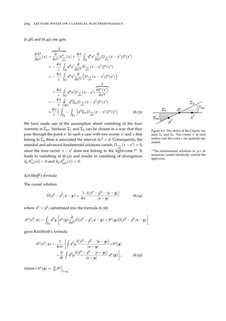
Figure 6.6: The choice of the Cauchy sur-faces S1 and S2. The events x0 at eachsurface and the event x are spatially sep-arated.
We have made use of the assumption about vanishing of the four-currents at S•. Surfaces S1 and S2 can be chosen in a way that theypass through the point x. In such a case with two events x0 and x thatbelong to Sk there is associated the interval Ds2 < 0. Consequently, theretarded and advanced fundamental solutions vanish, D ret
adv(x� x0) = 0,
since the four-vector x � x0 does not belong to the light-cone.10 It 10 The fundamental solutions in 3+1 di-mensions vanish identically outside thelight-cone.
leads to vanishing of (6.53) and results in vanishing of divergences∂µ Aµ
ret(x) = 0 and ∂µ Aµadv(x) = 0.
Kirchhoff’s formula
The causal solution
D(x0� y0, x� y) =
14p
d(x0 � y0 � |x� y|)|x� y|
(6.54)
where x0 > y0, substituted into the formula (6.36)
Aµ(x0, x) =Z
S0d3y
aµ(y)
∂
∂x0 D(x0� y0, x� y) + bµ(y)D(x0
� y0, x� y)
�
gives Kirchhoff’s formula
Aµ(x0, x) =1
4pc
Zd3y
d(x0 � y0 � |x� y|)|x� y|
c bµ(y)
+∂
∂t
Zd3y
d(x0 � y0 � |x� y|)|x� y|
aµ(y)
�, (6.55)
where c bµ(y) = ∂∂t Aµ
���t=t0
.
electromagnetic radiation 205
Cauchy problem in 1+1 dimensions
The general solution of inhomogeneous wave equation in 1+1 dimen-sions can be obtained even though the inhomogeneity is present at thesurface if initial data.
Since A0 and A1 obey the same equation, then it is sufficient toanalyze the problem of a scalar field obeying the inhomogeneous waveequation and initial conditions
utt � c2uxx = f (t, x)
u(0, x) = j(x), ut(0, x) = y(x).(6.56)
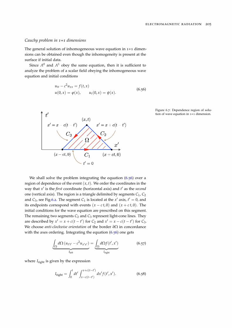
Figure 6.7: Dependence region of solu-tion of wave equation in 1+1 dimension.
We shall solve the problem integrating the equation (6.56) over aregion of dependence of the event (x, t). We order the coordinates in theway that x0 is the first coordinate (horizontal axis) and t0 as the secondone (vertical axis). The region is a triangle delimited by segments C1, C2
and C3, see Fig.6.2. The segment C1 is located at the x0 axis, t0 = 0, andits endpoints correspond with events (x� c t, 0) and (x + c t, 0). Theinitial conditions for the wave equation are prescribed on this segment.The remaining two segments C2 and C3 represent light-cone lines. Theyare described by x0 = x + c(t� t0) for C2 and x0 = x� c(t� t0) for C3.We choose anti-clockwise orientation of the border ∂W in concordancewith the axes ordering. Integrating the equation (6.56) one gets
Z
WdW (ut0t0 � c2ux0x0)
| {z }Ileft
=Z
WdW f (t0, x0)
| {z }Iright
(6.57)
where Iright is given by the expression
Iright =Z t
0dt0Z x+c(t�t0)
x�c(t�t0)dx0 f (t0, x0). (6.58)
206 lecture notes on classical electrodynamics
On the other hand, the expression Ileft can be evaluated applying Stokestheorem in two dimensions. Stokes theorem
Z
Wda · (r⇥ F) =
I
∂WF · dl
simplifies to the formZ
Wdy1dy2| {z }
dW
⇣∂1F2
� ∂2F1⌘=I
∂W
⇣F1dy1 + F2dy2
⌘(6.59)
where dy1 = dx0 and dy2 = dt0. The left hand side of the wave equationcan be cast in the following form
∂2t0u� c2∂2
x0u = ∂x0|{z}∂1
(�c2∂x0u)| {z }F2
� ∂t0|{z}∂2
(�∂t0u)| {z }F1
. (6.60)
Thus the integral Ileft can be replaced by the line integral taken alongthe border ∂W
Ileft =I
∂W(F1dy1 + F2dy2)
=I
∂W[�(∂t0u)dx0 � c2(∂x0u)dt0]
= I1 + I2 + I3,
where the integrals I1, I2, I3 are evaluated on the segments C1, C2, C3.
• Integral I1:dt0 = 0 along the line C1 and thus
I1 =Z x+ct
x�ctdx0[�∂t0u(t0, x0)]t0=0 = �
Z x+ct
x�ctdx0y(x0) (6.61)
• Integral I2:dx0 = �c dt0 along the light-cone C2. It gives
I2 =Z
C2[�(∂t0u)dx0 � c2(∂x0u)dt0]
=Z
C2
�(∂t0u)(�c dt0)� c2(∂x0u)
✓�
dx0
c
◆�
= cZ
C2[∂t0u dt0 + ∂x0u dx0]
= cZ
C2du
= c[u(t, x)� u(0, x + ct)] = c[u(t, x)� j(x + ct)]. (6.62)
• Integral I3:
electromagnetic radiation 207
dx0 = +c dt0 along the light-cone C3. It gives
I3 =Z
C3[�(∂t0u)dx0 � c2(∂x0u)dt0]
=Z
C3
�(∂t0u)(c dt0)� c2(∂x0u)
✓dx0
c
◆�
= �cZ
C3[∂t0u dt0 + ∂x0u dx0]
= �cZ
C3du
= �c[u(0, x� ct)� u(t, x)] = c[u(t, x)� j(x� ct)]. (6.63)
Plugging the obtained result into I1 + I2 + I3 = Iright we get
2cu(t, x)� c[j(x + ct) + j(x� ct)]�Z x+ct
x�ctdx0y(x0) =
=Z t
0dt0Z x+c(t�t0)
x�c(t�t0)dx0 f (t0, x0)
which gives
u(t, x) =12[j(x + ct) + j(x� ct)]
+12c
Z x+ct
x�ctdx0y(x0) +
12c
Z t
0dt0Z x+c(t�t0)
x�c(t�t0)dx0 f (t0, x0). (6.64)
Note that the last term can be also cast in the form
12c
Z t
0dt0Z x+c(t�t0)
x�c(t�t0)dx0 f (t0, x0) =
=Z
R2dt0dx0
12c
q⇣
c(t� t0)� |x� x0|⌘�
| {z }D(1)
ret (t�t0 ,x�x0)
f (t0, x0), (6.65)
where we define
D(1)ret (t, x) :=
12c
q(ct� |x|).
208 lecture notes on classical electrodynamics
6.3 Radiation field from a moving particle
In this section we pay attention to description of electromagnetic fieldfrom electrically charged particle in motion. First we derive the elec-tromagnetic strength tensor and then obtain the associated energymomentum tensor. In further part we discuss the braking radiation.Finally we study radiation generated by large group of charges.
Radiation field
A radiation field is defined as the difference between outgoing andincoming fields. The radiation field in terms of four-potentials Aµ
out(x)and Aµ
in(x) reads
Aµrad(x) := Aµ
out(x)� Aµin(x), (6.66)
where Aµout(x) is the electromagnetic four-potential in remote future and
Aµin(x) is the four-potential in remote past. The equality (6.50) allows us
to put the radiation field in dependence on the retarded and advancedfour-potentials
Aµrad(x) = Aµ
ret(x)� Aµadv(x)
=4p
c
Zd4x0
hDret(x� x0)� Dadv(x� x0)
iJµ(x0)
=4p
c
Zd4x0 D(x� x0)Jµ(x0), (6.67)
where D(x� x0) is defined in (6.22). Note that, (6.66) and (6.67) leadsto relation Scattering problem
Aµout(x) = Aµ
in(x) +4p
c
Zd4x0 D(x� x0)Jµ(x0) (6.68)
which is a relation between asymptotic states of the electromagneticfield. Unlike the asymptotic fields, the disturbance represented byR
d4x0 D(x� x0)Jµ(x0) appears for finite times. Hence the expression(6.68) gives a relationship between two asymptotic states for the scatter-ing process
Aµout(x) = SAµ
in(x),
where S is the counterpart of the scattering matrix.The electromagnetic field tensor Fµn = ∂µ An � ∂n Aµ takes the fol-
lowing form
Fradµn (x) =
4p
c
Zd4x0
"∂D(x� x0)
∂xµ Jn(x0)�∂D(x� x0)
∂xn Jµ(x0)
#(6.69)
where Aµ is given by (6.67).
electromagnetic radiation 209
Lienard-Wichert potentials
The simplest physical system containing electromagnetic radiationwhich can be described exactly is a point-like charged particle followingsome world-line. In the first stage we shall assume that the particleworld line is given by the prescribed (explicitly given) curve. Theparticle in non-uniform motion is represents a forced physical system.11 11 It requires an external power source
to maintain a prescribed motion of theparticle.
Thus we pay attention on kinematics but not dynamics of the particle.The particle dynamics in the presence of external electromagnetic fieldis studied in further part of this chapter. In such a case the particleworld-line is determined by two factors: its interaction with the externalfield and the radiation process.
At the present stage we shall assume that the world-line of thecharged particle is explicitly given – described by the four vector zµ(t).The electric four-current density of the particle reads Four-current density of of a sin-
gle point-like charged particleJµ(x) = qc
Z •
�•dt
dzµ
dtd4(x� z(t)). (6.70)
This four-current vanishes in everywhere except the world-line of theparticle. With the help of (6.70) one gets the retarded (advanced) four-potentials
Aµretadv
(x) =4p
c
Zd4x0D ret
adv(x� x0)Jµ(x0)
=4p
cqc2p
Zd4x0
Z •
�•dt q
⇣± (x0
� x00)⌘
dh(x� x0)2
i⇥
⇥dzµ
dtd4(x0 � z(t))
=2qZ •
�•dt q
⇣± (x0
� z0)⌘dzµ
dtdh(x� z(t))2
i. (6.71)
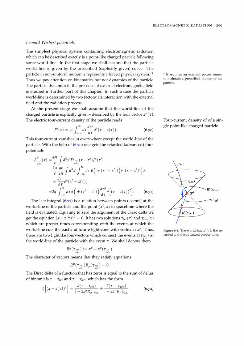
Figure 6.8: The world-line zµ(t); the re-tarded and the advanced proper time.
The last integral (6.71) is a relation between points (events) at theworld-line of the particle and the point (x0, x) in spacetime where thefield is evaluated. Equating to zero the argument of the Dirac delta weget the equation (x� z(t))2 = 0. It has two solutions tret(x) and tadv(x)which are proper times corresponding with the events at which theworld-line cuts the past and future light-cone with vertex at xµ. Thus,there are two lightlike four-vectors which connect the events z(t ret
adv) at
the world-line of the particle with the event x. We shall denote them
Rµ(t retadv
) := xµ� zµ(t ret
adv).
The character of vectors means that they satisfy equations
Rµ(t retadv
)Rµ(t retadv
) = 0.
The Dirac delta of a function that has zeros is equal to the sum of deltasof binomials t � tret and t � tadv which has the form
dh(x� z(t))2
i=
d(t � tret)|� 2zµRµ|tret
+d(t � tadv)
|� 2zµRµ|tadv
(6.72)
210 lecture notes on classical electrodynamics
Plugging (6.72) into (6.71) one gets
Aµretadv
(x) = qZ •
�•zµq⇣± (x0
� z0(t))⌘ d(t � tret)
|zµRµ|tret+
d(t � tadv)|zµRµ|tadv
�
= q q⇣± (x0
� z0(tret))⌘ zµ(tret)|zµRµ|tret
+
+ q q⇣± (x0
� z0(tadv))⌘ zµ(tadv)|zµRµ|tadv
.
Taking into account the identities
q⇣+ (x0
� z0(tret))⌘= 1, q
⇣� (x0
� z0(tadv))⌘= 1,
q⇣+ (x0
� z0(tadv))⌘= 0, q
⇣� (x0
� z0(tret))⌘= 0,
and the inequalities zµRµ(tret) > 0, zµRµ(tadv) < 0 one gets Lienart- Lienard-Wichert potentialsWichert potentials
Aµretadv
(x) = ±qzµ
Ra za
����t ret
adv(x)
=qc
zµ
r
����t ret
adv(x)
(6.73)
where we have denoted
r retadv
:=1c
���(xa� za(t ret
adv))za(t ret
adv)��� ⌘ ±
1c
Ra za
���t ret
adv(x)
. (6.74)
The expression r(x) has interpretation of spatial distance between theevents x and z(t ret
adv). In the instantaneous rest frame
r(x)���
IR= ±
1c(x0� z0)
��� retadv
c = |x� z|.
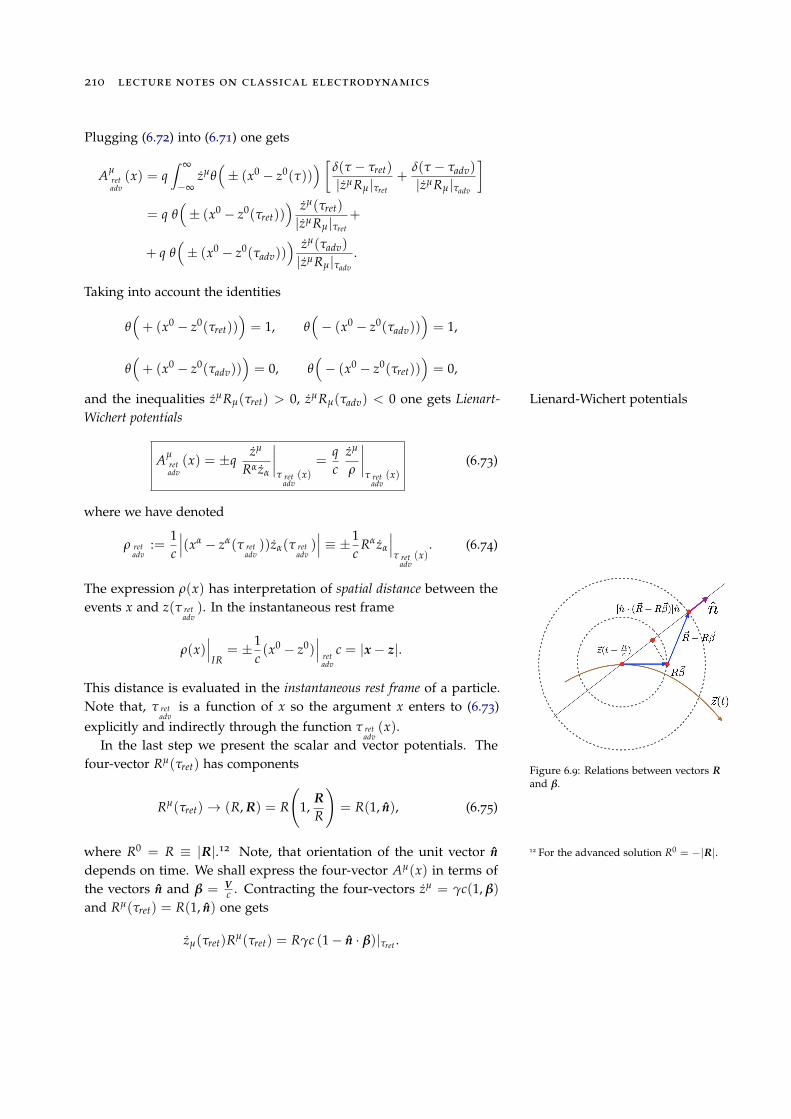
Figure 6.9: Relations between vectors R
and b.
This distance is evaluated in the instantaneous rest frame of a particle.Note that, t ret
advis a function of x so the argument x enters to (6.73)
explicitly and indirectly through the function t retadv
(x).In the last step we present the scalar and vector potentials. The
four-vector Rµ(tret) has components
Rµ(tret)! (R, R) = R
1,
R
R
!= R(1, n), (6.75)
where R0 = R ⌘ |R|.12 Note, that orientation of the unit vector n 12 For the advanced solution R0 = �|R|.
depends on time. We shall express the four-vector Aµ(x) in terms ofthe vectors n and b = V
c . Contracting the four-vectors zµ = gc(1, b)
and Rµ(tret) = R(1, n) one gets
zµ(tret)Rµ(tret) = Rgc (1� n · b)|tret .
electromagnetic radiation 211
The relation between t0 and t follows from the component R0(tret) =
ct� ct0(tret) and it reads
t0(tret) = t�Rc
.
Thus, the retarded electromagnetic potentials can be expressed in theform The retarded scalar potential and
the vector potentialA0(t, x) =
qR
11� n · b
����t� R
c
,
A(t, x) =qR
b
1� n · b
����t� R
c
. (6.76)
The field tensor
The electromagnetic field tensor is given in terms of the retarded (ad-vanced) potentials (6.73)
Fretadv
µn (x) = ∂µ
qzn
cr
�
t(x)� ∂n
qzµ
cr
�
t(x), (6.77)
where t(x) ⌘ t retadv
(x) is a function of x. For further convenience wedefine the symbol
(ab) := aaba.
The first term of (6.77) reads za = za(t(x))
∂µ Aretadvn (x) =
qc
1r
∂µ zn �1r2 ∂µr zn
�(6.78)
where partial derivatives of za = za(t(x)) contains derivatives of t(x)according to ∂za
∂xµ = dza
dt
���t(x)
∂t(x)∂xµ . In particular, the derivative ∂µr reads
∂µr =∂µ
⇣±
1c
Ra za|t(x)
⌘
=±1c⇥∂µ(xa
� za)za + Ra∂µ za⇤
=±1c
h(da
µ � za∂µt(x))za + Ra za∂µt(x)i
=±1c
hzµ +
⇣(Rz)� c2
⌘∂µt(x)
i. (6.79)
The expression ∂µt(x) follows from the equation ∂µ(RaRa) = 0 whichgives
(daµ � za∂µt(x))Ra = 0.
Thus, ∂µt(x) reads Expression ∂µt retadv
(x)
∂µt(x) =Rµ
(Rz)= ±
Rµ
c r=: ±kµ ) Rµ = crkµ, (6.80)
212 lecture notes on classical electrodynamics
where kµ zµ = ±1, kµkµ = 0. The labels ret, adv have been omitted for The lightlike four-vector kµ:
kµ zµ = ±1, kµkµ = 0simplicity. Hence
Rµ⌘ Rµ
retadv
, r ⌘ r retadv
, kµ⌘ kµ
retadv
.
Taking into account (6.80) one gets (6.79) in the form
∂µr = ±1c
zµ +hr (kz)� c
ikµ. (6.81)
Substituting this result into (6.78) one gets
∂µ Aretadvn =
qc
1r(±kµ zn)�
1c r2 (±zµ zn)�
1r2 (r (kz)� c) kµ zn
�
= qkµ
zn
r2 +±zn � (kz)zn
c r
�⌥
qc2
zµ zn
r2 . (6.82)
The term containing zµ zn does not contribute to the electromagneticfield tensor because it is symmetric in its indices µ and n. This tensortakes the form The electromagnetic field tensor
Fretadv
µn (x) = kµxn � knxµ (6.83)
where
xn := q
zn
r2 +±zn � (kz)zn
c r
�. (6.84)
The tensor (6.83) can be split into two terms
Fretadv
µn (x) = F(1)µn (x) + F(2)
µn (x)
where
F(1)µn (x) =
qr2 (kµ zn � kn zµ), (6.85)
F(2)µn (x) =
qc r
h± (kµ zn � kn zµ)� (kz)(kµ zn � kn zµ)
i. (6.86)
The Coulomb fieldNote that the expression F(1)
µn (x) does not contain second derivativeswith respect to proper time (independence on acceleration). To haveinsight into its physical meaning we assume zµ = const. In such a casezµ = 0 and the electromagnetic field is given by the first term
Fretadv
µn (x) = F(1)µn (x).
We take a space-like four-vector wµ such that w2 < 0
wµ zµ = 0, wµwµ = �c2. (6.87)
The light-like four-vector kµ can be written in the from
kµretadv
=1c2 (±zµ + wµ) (6.88)
electromagnetic radiation 213
where the sign “+” stands for the retarded function and “�” for theadvanced one. Substituting the expression (6.88) into (6.85) one gets
F(1)µn (x) =
qc2 r2 (zµwn � znwµ) (6.89)
where the retarded and advanced distance have equal values, rret =
radv ⌘ r. The four-vectors zµ and wµ in the instantaneous rest frame of aparticle read
zµ = (c, 0), wµ = (0, c n).
Thus the tensor F(1)µn represents the Coulomb field associated with a
charged particle The Coulomb field
F(1)0i =
q ni
r2 , F(1)ij = 0.
The particle which moves without acceleration is surrounded by afield which is proportional to ⇠ r�2. This is the proper field from acharged particle. Note that the electromagnetic field tensors (6.89) forthe retarded and advanced solutions are equal The proper field from a parti-
cle does not contribute to elec-tromagnetic radiationF(1)ret
µn = F(1)advµn .
This field does not contribute to electromagnetic radiation given by
Fradµn = Fret
µn � Fadvµn = F(1)ret
µn � F(1)advµn = 0.
The total fieldIn what follows, we look at total electromagnetic field which contains
terms proportional to acceleration of the particle. We express all theformulas with the help of four-vector nµ defined as follows
Rµ⌘ Rnµ
! R(±1, n)
where R ⌘ |R| and n2 = 1. It gives
kµretadv
= ±Rµ
(Rz)= ±
nµ
(nz)and r ret
adv= ±
1c(Rz) = ±
Rc(nz).
Thus, the expression (6.84) can be cast in the form
xn = q
zn
r2 +±zn � (kz)zn
c r
�
= q
2
4 zn
R2
c2 (nz)2+
±
⇣zn �
(nz)(nz) zn
⌘
±R(nz)
3
5
=qc2
R2zn
(nz)2 +qR(nz)zn � (nz)zn
(nz)2 . (6.90)
The electromagnetic field tensor Fretadv
µn = F(1)µn + F(2)
µn is given in terms ofexpressions The components of the electro-
magnetic tensor of a charged par-ticle in non-uniform motion
214 lecture notes on classical electrodynamics
F(1)µn = ±
qc2
R2nµ zn � nn zµ
(nz)3
���� retadv
, (6.91)
F(2)µn = ±
qR(nz)(nµ zn � nn zµ)� (nz)(nµ zn � nn zµ)
(nz)3
����� retadv
. (6.92)
The part of the electromagnetic field tensor (6.91) proportional toR�2 has been already recognized as the Coulomb field from the chargedparticle. It is said that there is no external free field if the electromag-netic field surrounding the charged particle is equal to its Coulombfield.
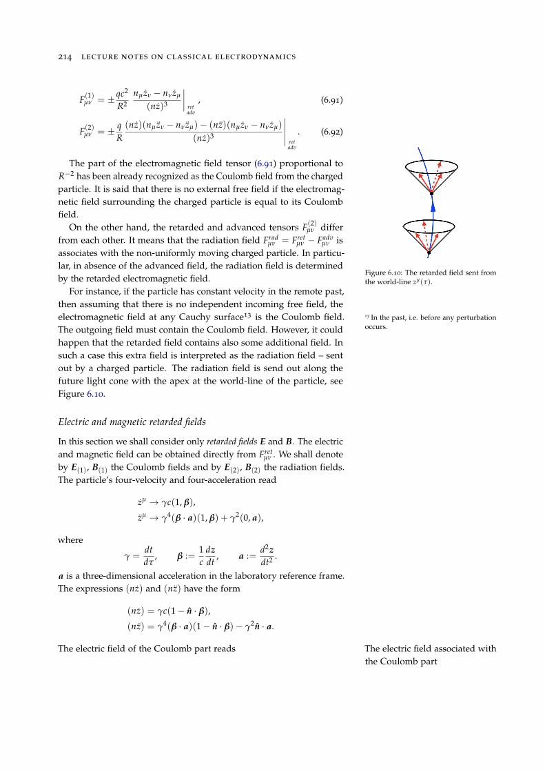
Figure 6.10: The retarded field sent fromthe world-line zµ(t).
On the other hand, the retarded and advanced tensors F(2)µn differ
from each other. It means that the radiation field Fradµn = Fret
µn � Fadvµn is
associates with the non-uniformly moving charged particle. In particu-lar, in absence of the advanced field, the radiation field is determinedby the retarded electromagnetic field.
For instance, if the particle has constant velocity in the remote past,then assuming that there is no independent incoming free field, theelectromagnetic field at any Cauchy surface13 is the Coulomb field. 13 In the past, i.e. before any perturbation
occurs.The outgoing field must contain the Coulomb field. However, it couldhappen that the retarded field contains also some additional field. Insuch a case this extra field is interpreted as the radiation field – sentout by a charged particle. The radiation field is send out along thefuture light cone with the apex at the world-line of the particle, seeFigure 6.10.
Electric and magnetic retarded fields
In this section we shall consider only retarded fields E and B. The electricand magnetic field can be obtained directly from Fret
µn . We shall denoteby E(1), B(1) the Coulomb fields and by E(2), B(2) the radiation fields.The particle’s four-velocity and four-acceleration read
zµ! gc(1, b),
zµ! g4(b · a)(1, b) + g2(0, a),
where
g =dtdt
, b :=1c
dz
dt, a :=
d2z
dt2 .
a is a three-dimensional acceleration in the laboratory reference frame.The expressions (nz) and (nz) have the form
(nz) = gc(1� n · b),
(nz) = g4(b · a)(1� n · b)� g2n · a.
The electric field of the Coulomb part reads The electric field associated withthe Coulomb part
electromagnetic radiation 215
Ei(1) = Fi0
(1) =qc2
R2niz0 � n0zi
(nz)3
����t� R
c
=qc2
R2gcni � gvi
g3c3(1� n · b)3
����t� R
c
=q
R2 (1� b2)ni � bi
(1� n · b)3
����t� R
c
, (6.93)
where the retarded time in the laboratory reference frame is given bythe expression
tret = t�Rc
.
The magnetic field has the form The magnetic field associatedwith the Coulomb part
Bi(1) = �
12
eijkFjk(1) = �
12
eijkqc2
R2njzk � nkzj
(nz)3
�����t� R
c
= �eijkqc2
R2njzk
(nz)3
�����t� R
c
=q
R2 (1� b2)eijknj(�bk)
(1� n · b)3
�����t� R
c
=q
R2 (1� b2)eijknj(nk � bk)
(1� n · b)3
�����t� R
c
= (n⇥ E(1))i���t� R
c. (6.94)
The magnetic field (6.94) is perpendicular to the electric field (6.93) andits magnitude is proportional to magnitude of the electric field.
The electric field which depends on the acceleration is given byexpression The electric part of the radiation
fieldEi(2) = Fi0
(2) =qR(nz)(niz0 � n0zi)� (nz)(niz0 � n0zi)
(nz)3
����t� R
c
=qR[(nz)z0 � (nz)z0]ni � [(nz)zi � (nz)zi]
(nz)3
����t� R
c
. (6.95)
Substituting expressions
(nz)z0� (nz)z0 = gc(1� n · b) [g4(b · a)]
� [g4(b · a)(1� n · b)� g2n · a]gc
= g3c n · a (6.96)
and
(nz)zi� (nz)zi = gc(1� n · b)[⇠⇠⇠⇠⇠
g4(b · a)bi + g2ai]
� [(((((((((g4(b · a)(1� n · b)� g2(n · a)]gcbi
= g3c [(n · a)bi + (1� n · b)ai] (6.97)
216 lecture notes on classical electrodynamics
into the formula (6.95) one gets
Ei(2) =
qR
g3c (n · a)ni � g3c [(n · a)bi + (1� n · b)ai]g3c3(1� n · b)3
����t� R
c
=q
Rc2(n · a)(ni � bi)� n · (n� b)ai
(1� n · b)3
����t� R
c
=q
Rc2(n⇥ [(n� b)⇥ a])i
(1� n · b)3
����t� R
c
. (6.98)
The electric field (6.98) has origin in accelerated motion of the chargedparticle, a 6= 0.
Finally, the magnetic field takes the form The magnetic field associatedwith the radiation part
Bi(2) = �
12
eijkFjk(2)
= �12
qR
eijk(nz)[njzk � nkzj]� (nz)[njzk � nkzj]
(nz)3
�����t� R
c
= �qR
eijk(nz)[njzk]� (nz)[njzk]
(nz)3
�����t� R
c
=qR
eijknj[(nz)zk � (nz)zk]
(nz)3
�����t� R
c
(6.97)=
qR
eijknj g3c [(n · a)(�bk)� (1� n · b)ak]g3c3(1� n · b)3
�����t� R
c
=q
Rc2 eijknj (n · a)(nk � bk)� n · (n� b)ak
(1� n · b)3
�����t� R
c
=q
Rc2
n⇥
n⇥ [(n� b)⇥ a](1� n · b)3
�i�����t� R
c
= [n⇥ E(2)]i���t� R
c. (6.99)
To summarize our results we define the vector Summary
K :=n� b
(1� n · b)3 (6.100)
which allows us to put (6.93), (6.94), (6.98) and (6.99) in the followingform
E(1) =q
R2 (1� b2)K���t� R
c, B(1) = n⇥ E(1), (6.101)
E(2) =q
Rc2 n⇥ (K ⇥ a)|t� Rc
, B(2) = n⇥ E(2). (6.102)
It follows from these expressions that the total magnetic field is a crossproduct of n and the total electric field E = E(1) + E(2).
electromagnetic radiation 217
The Coulomb field
In this section we show the equivalence of two expressions for theCoulomb field from the charged particle. This expressions are obtainedwith the help of retarded potentials and, alternatively, as the Lorentzboost of the electrostatic field surrounding a charged particle.
According to our previous considerations, the Lorentz transforma-tion of the electrostatic field from a point charge reads
E(t, x) = qR0
R031� b2
(1� b2 sin2 J0)3/2, B = b⇥ E (6.103)
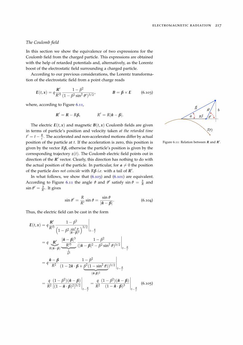
where, according to Figure 6.11,
R0 = R� Rb, R0 = R|n� b|.
Figure 6.11: Relation between R and R0.
The electric E(t, x) and magnetic B(t, x) Coulomb fields are givenin terms of particle’s position and velocity taken at the retarded timet0 = t� R
c . The accelerated and non-accelerated motions differ by actualposition of the particle at t. If the acceleration is zero, this position isgiven by the vector Rb, otherwise the particle’s position is given by thecorresponding trajectory z(t). The Coulomb electric field points out indirection of the R
0 vector. Clearly, this direction has nothing to do withthe actual position of the particle. In particular, for a 6= 0 the positionof the particle does not coincide with Rb i.e. with a tail of R
0.In what follows, we show that (6.103) and (6.101) are equivalent.
According to Figure 6.11 the angle J and J0 satisfy sin J = bR and
sin J0 = bR0 . It gives
sin J0 =RR0
sin J =sin J
|n� b|. (6.104)
Thus, the electric field can be cast in the form
E(t, x) = qR0
R031� b2
⇣1� b2 sin2 J
|n�b|2
⌘3/2
�����t� R
c
= q R0
|{z}R(n�b)
|n� b|3
R03| {z }1
R3
1� b2
(|n� b|2 � b2 sin2 J)3/2
�����t� R
c
= qn� b
R21� b2
(1� 2n · b + b2(1� sin2 J)| {z }
(n·b)2
)3/2
�����t� R
c
=q
R2(1� b2)(n� b)
[(1� n · b)2]3/2
�����t� R
c
=q
R2(1� b2)(n� b)(1� n · b)3
�����t� R
c
(6.105)
218 lecture notes on classical electrodynamics
Thus the electric field has the form (6.101). The magnetic field is aconsequence of (6.105) and the equality
b⇥ (n� b) = b⇥ n = �n⇥ b = n⇥ (n� b). (6.106)
It readsB(t, x) = n⇥ E
���t� R
c
. (6.107)
Thus, in the case of uniform motion both formulas are equivalent. Theretarded potentials, however, give deeper insight into the problem.
Radiated power
Emission of radiation is a process in which an accelerated particle loosesits energy. This emission is described by energy flux which representsthe amount of energy per unit of time emitted in the solid angle dW inthe direction of n. The energy emitted during infinitesimal time intervaldt0 is given by dP(t0)dt0, where dP(t0) stands for radiated power.14 This 14 More precisely, it is a power distribu-
tion.
Radiated powerpower is a function of angles parametrising vector n. We denote by dt0
the interval in which certain infinitesimal amount of energy is emittedand by dt the interval in which this amount of energy is registered–pass through the infinitesimal area da = nR2dW. Since both energiesare equal, then Equality of energies emitted by
the particle and registered in thelaboratory reference frame
dP(t0)dt0 = dP(t)dt. (6.108)
Instants of time t0 and t are related by the expression
t = t0 +1c
R(t0) (6.109)
where t0 and t stand, respectively, for emission and registration instantsof time (E(t) and B(t) are evaluated at t). The expression (6.109) leadsto the relation
dtdt0
= 1 +1c
dR(t0)dt0
.
Taking the derivative of R(t0)2 = R(t0) · R(t0) with respect to t0 onegets
���2R(t0)dR(t0)
dt0=���2R(t0)n(t0) ·
dR(t0)dt0
where R(t0) = x� z(t0) = R(t0)n(t0). It leads to the expression
dR(t0)dt0
= n(t0) ·d
dt0(x� z(t0)) = �n(t0) · v(t0) = �c n(t0) · b(t0).
The relation between the time intervals dt0 and dt reads Relation between the intervalsdt0 and dt
dtdt0
= 1� n · b (6.110)
electromagnetic radiation 219
where n · b is taken at the retarded time t0. This expression allows usto get the radiated power P(t0) in terms of the power measured at thesphere with radius R.15 Comparing the expression 15 Note, that the fields are singular at the
position of a charged particle, hence thePoynting vector is also singular at theparticle.
dP(t)dt =
dP(t)dtdt0
�dt0 = dP(t0)dt0 (6.111)
with (6.108) one gets the radiated power The radiated power in terms ofthe registered powerdP(t0) = (1� n · b)dP(t). (6.112)
The registered power distribution dP(t) can be expressed in terms ofthe Poynting vector S(t) and it has the form
dP(t) = S(t) · da = S(t) · n R2dW (6.113)
where The Poynting vector
S(t) =c
4pE⇥ B =
c4p
hE⇥ (n⇥ E)
i=
c4p
hn E
2� (n · E)2
i. (6.114)
Since the electric field E satisfies16E · n = 0, then 16 Here E ⌘ E(2). We omit the Coulomb
component because it behaves as R�2 soit became irrelevand far from the radia-tion source.
dP(t) =c
4pE
2R2dW =c
4pR2 q2
R2c4
hn⇥ (K ⇥ a)
i2����t� R
c
dW
=q2
4pc3
h(n · a)K � (n · K)a
i2���t� R
c
dW
=q2
4pc3
h(n · a)2
K2 + (n · K)2
a2� 2(n · a)(n · K)(a · K)
i
t� Rc
dW.
(6.115)
Substituting K given by (6.100) into (6.115) one gets
dP(t) =q2
4pc31
(1� n · b)6 [(n · a)2(n� b)2 + (1� n · b)2a
2
� 2(n · a)(1� n · b)(n · a� b · a)]t� Rc
dW
=q2
4pc31
(1� n · b)6
"(n · a)2 (1 + b2
� 2n · b)| {z }�(1�b2)+⇠⇠⇠⇠2(1�n·b)
+(1� n · b)2a
2
�(((((((((2(n · a)2(1� n · b) + 2(n · a)(1� n · b)(n · b)
#
t� Rc
dW.
(6.116)
Finally, substituting (6.116) into (6.112) we get angular distribution ofthe radiated power Angular distribution of the radi-
ated powerdP(t0) =
q2
4pc3 W(t0, n)dW (6.117)
where
W(t0, n) :=
a2
(1� n · b)3 + 2(n · a)(b · a)
(1� n · b)4 � (1� b2)(n · a)2
(1� n · b)5
�
t� Rc
.
(6.118)
220 lecture notes on classical electrodynamics
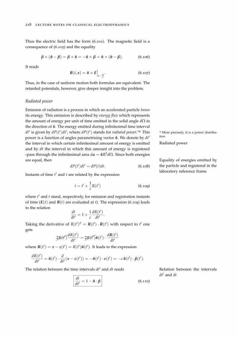
Acceleration parallel to velocity
In this section we look at the case of mutually parallel velocity andacceleration of the particle i.e. b⇥ a = 0. The electric field (6.102) isproportional to
Figure 6.12: The angular distribution ofthe radiated power for b = 0.1.
Figure 6.13: The angular distribution ofthe radiated power for b = 0.5.
Figure 6.14: The angular distribution ofthe radiated power for b = 0.8.
n⇥ (K ⇥ a) =n⇥ (n⇥ a)(1� n · b)3 =
(n · a)n� a
(1� n · b)3 .
The power distribution (6.117) reads
dP(t0) =q2
4pc3a
2 � (n · a)2
(1� n · b)5
����t� R
c
dW. (6.119)
Let z be a versor parallel to b, defined as z := b/b. The accelerationreads a = az. We introduce spherical coordinates where J in an anglebetween n and z, hence n · a = a cos J. The power radiated into theinfinitesimal solid angle dW = sin J dJ dj reads
dP(t0) =q2
4pc3a2 sin2 J
(1� b cos J)5
�����t� R
c
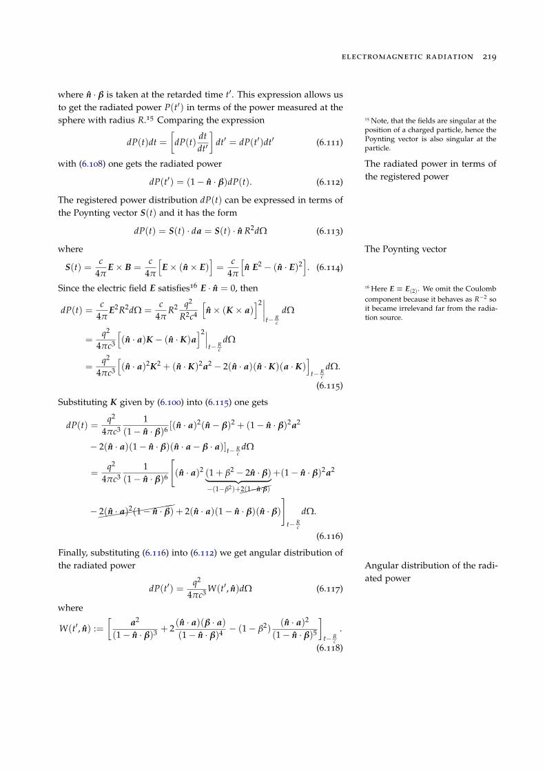
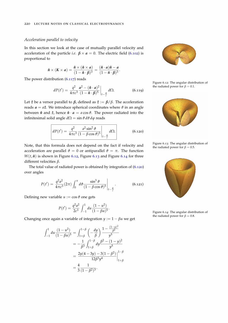
dW. (6.120)
Note, that this formula does not depend on the fact if velocity andacceleration are parallel J = 0 or antiparallel J = p. The functionW(t, n) is shown in Figure 6.12, Figure 6.13 and Figure 6.14 for threedifferent velocities b.
The total value of radiated power is obtained by integration of (6.120)over angles
P(t0) =q2a2
4pc3 (2p)Z p
0dJ
sin3 J
(1� b cos J)5
�����t� R
c
. (6.121)
Defining new variable u := cos J one gets
P(t0) =q2a2
2c3
Z 1
�1du
(1� u2)(1� bu)5 .
Changing once again a variable of integration y := 1� bu we get
Z 1
�1du
(1� u2)(1� bu)5 =
Z 1�b
1+b
✓�
dyb
◆ 1� (1�y)2
b2
y5
= �1b3
Z 1�b
1+bdy
b2 � (1� y)2
y5
=2y(4� 3y)� 3(1� b2)
12b3y4
����1�b
1+b
=43
1(1� b2)3 .
electromagnetic radiation 221
Thus, the total radiated power reads
P(t0) =2q2
3c3a2
(1� b2)3
����t� R
c
⇠ g6. (6.122)
For small velocities the last formula simplifies to the following one
P(t0) =23
q2a2
c3 . (6.123)
Acceleration perpendicular to velocity
Now we look at the case of acceleration perpendicular to velocity i.e.b · a = 0. The radiated power distribution can be obtained directlyfrom (6.117) and (6.118). It reads
dP(t0) =q2
4pc3
a
2
(1� n · b)3 � (1� b2)(n · a)2
(1� n · b)5
�
t� Rc
dW. (6.124)
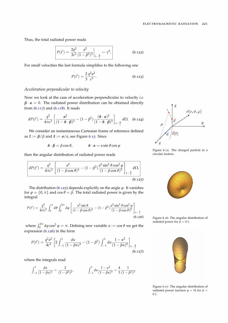
Figure 6.15: The charged particle in acircular motion.
We consider an instantaneous Cartesian frame of reference definedas z := b/b and x := a/a, see Figure 6.15. Since
n · b = b cos J, n · a = a sin J cos j
then the angular distribution of radiated power reads
dP(t0) =q2
4pc3
"a2
(1� b cos J)3 � (1� b2)a2 sin2 J cos2 j
(1� b cos J)5
#
t� Rc
dW.
(6.125)
Figure 6.16: The angular distribution ofradiated power for b = 0.1.
Figure 6.17: The angular distribution ofradiated power (section j = 0) for b =0.1.
The distribution (6.125) depends explicitly on the angle j. It vanishesfor j = {0, p} and cos J = b. The total radiated power is given by theintegral
P(t0) =q2
4pc3
Z p
0dJZ 2p
0dj
"a2 sin J
(1� b cos J)3 � (1� b2)a2 sin3 J cos2 j
(1� b cos J)5
#
t� Rc
(6.126)
whereR 2p
0 dj cos2 j = p. Defining new variable u := cos J we get theexpression (6.126) in the form
P(t0) =q2a2
4c3
2Z 1
�1
du(1� bu)3 � (1� b2)
Z 1
�1du
1� u2
(1� bu)5
�
t� Rc
(6.127)
where the integrals readZ 1
�1
du(1� bu)3 =
2(1� b2)2 ,
Z 1
�1du
1� u2
(1� bu)5 =43
1(1� b2)3 .
222 lecture notes on classical electrodynamics
The total radiated power has the form
P(t0) =2q2
3c3a2
(1� b2)2
����t� R
c
⇠ g4. (6.128)
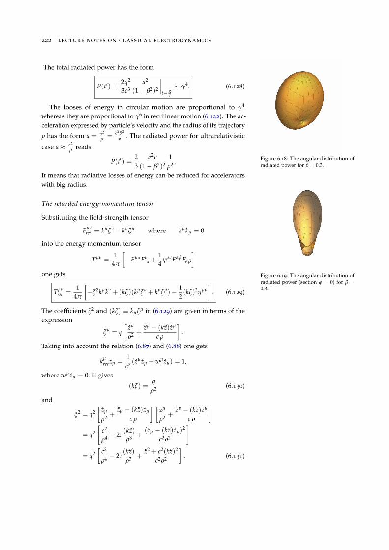
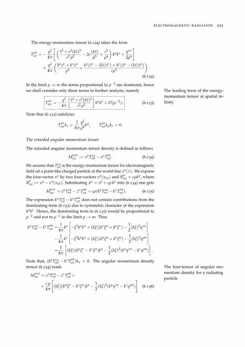
Figure 6.18: The angular distribution ofradiated power for b = 0.3.
Figure 6.19: The angular distribution ofradiated power (section j = 0) for b =0.3.
The looses of energy in circular motion are proportional to g4
whereas they are proportional to g6 in rectilinear motion (6.122). The ac-celeration expressed by particle’s velocity and the radius of its trajectoryr has the form a = v2
r = c2b2
r . The radiated power for ultrarelativistic
case a ⇡ c2
r reads
P(t0) =23
q2c(1� b2)2
1r2 .
It means that radiative losses of energy can be reduced for acceleratorswith big radius.
The retarded energy-momentum tensor
Substituting the field-strength tensor
Fµnret = kµxn
� knxµ where kµkµ = 0
into the energy momentum tensor
Tµn =1
4p
�FµaFn
a +14
hµnFabFab
�
one gets
Tµnret =
14p
�x2kµkn + (kx)(kµxn + knxµ)�
12(kx)2hµn
�. (6.129)
The coefficients x2 and (kx) ⌘ kµxµ in (6.129) are given in terms of theexpression
xµ = q
zµ
r2 +zµ � (kz)zµ
c r
�.
Taking into account the relation (6.87) and (6.88) one gets
kµretzµ =
1c2 (z
µ zµ + wµ zµ) = 1,
where wµ zµ = 0. It gives
(kx) =qr2 (6.130)
and
x2 = q2
zµ
r2 +zµ � (kz)zµ
c r
� zµ
r2 +zµ � (kz)zµ
c r
�
= q2
"c2
r4 � 2c(kz)r3 +
(zµ � (kz)zµ)2
c2r2
#
= q2
c2
r4 � 2c(kz)r3 +
z2 + c2(kz)2
c2r2
�. (6.131)
electromagnetic radiation 223
The energy-momentum tensor (6.129) takes the form
Tµnret =�
q2
4p
"✓z2 + c2(kz)2
c2 r2 � 2c(kz)r3 +
c2
r4
◆kµkn +
hµn
2r4
#
+q2
4p
✓kµ zn + kn zµ
r4 +kµ(zn � (kz)zn) + kn(zµ � (kz)zµ)
cr3
◆.
(6.132)
In the limit r! • the terms proportional to r�2 are dominant, hencewe shall consider only these terms in further analysis, namely The leading term of the energy-
momentum tensor at spatial in-finityTµn
ret = �q2
4p
z2 + c2(kz)2
c2 r2
�kµkn +O(r�3). (6.133)
Note that (6.132) satisfyies
Tµnret kn =
18p
q2
r4 kµ, Tµnret kµkn = 0.
The retarded angular momentum tensor
The retarded angular momentum tensor density is defined as follows
Mµnaret := xµTna
ret � xnTµaret . (6.134)
We assume that Tnaret is the energy-momentum tensor for electromagnetic
field od a point-like charged particle at the world-line zµ(t). We expressthe four-vector xµ by two four-vectors zµ(tret) and Rµ
ret = crkµ, whereRµ
ret := xµ � zµ(tret). Substituting xµ = zµ + cr kµ into (6.134) one gets
Mµnaret = zµTna
ret � znTµaret + cr(kµTna
ret � knTµaret ). (6.135)
The expression kµTnaret � knTµa
ret does not contain contributions from thedominating term (6.133) due to symmetric character of the expressionkµkn. Hence, the dominating term in (6.135) would be proportional tor�2 and not to r�1 in the limit r! •. Thus
kµTnaret � knTµa
ret =1
4pkµ�x2knka + (kx)(knxa + kaxn)�
12(kx)2hna
�
�1
4pkn�x2kµka + (kx)(kµxa + kaxµ)�
12(kx)2hµa
�
=1
4p
(kx)(kµxn
� knxµ)ka�
12(kx)2(kµhna
� knhµa)
�.
Note that, (kµTnaret � knTµa
ret )ka = 0. The angular momentum densitytensor (6.134) reads The four-tensor of angular mo-
mentum density for a radiatingparticle
Mµnaret = zµTna
ret � znTµaret+
+c r
4p
"(kx)(kµxn
� knxµ)ka�
12(kx)2(kµhna
� knhµa)
#(6.136)
224 lecture notes on classical electrodynamics
The expression (6.136) can be put in the form with explicit dependenceon four-velocity and four-acceleration of the particle. It takes the form
Mµnaret = zµTna
ret � znTµaret+
+q2c4p
kµ zn � kn zµ
r3 +kµ(zn � (kz)zn)� kn(zµ � (kz)zµ)
cr2
�ka
�q2c8p
kµhna � knhµa
r3 . (6.137)
Thus, the leading term of the angular-momentum tensor behaves asr�2 at spatial infinity The leading term of the angular
momentum density tensor at spa-tial infinity
Mµnaret = zµTna
ret � znTµaret+
+q2
4p
kµ(zn � (kz)zn)� kn(zµ � (kz)zµ)r2 ka +O(r�3) (6.138)
where
zµTnaret � znTµa
ret = �q2
4p
z2 + c2(kz)2
c2 r2
�(zµkn
� znkµ)ka +O(r�3).
6.4 Braking radiation (Bremsstrahlung)
In this section we study a charged particle in external electromagneticfield. We take into account the radiative loses of the four-momentumand the angular momentum. The solution of this problem requiresknowledge of the form of the energy-momentum tensor and the angular-momentum density tensor. It turns out that only the dominating termsfar from the particle are relevant. Finally, we derive relativistic equationof motion for the particle.
Four-momentum and angular momentum carried by electromagneticradiation
In what follows, we evaluate infinitesimal four-momentum dPµ andangular momentum dMµn carried by electromagnetic radiation. In-tegrating these expressions over angles we are able to get total four-momentum and total angular momentum which carried by radiation.
These quantities are evaluated in an inertial reference frame S0 that Asymptotic relationsmoves along the world-line
yµ(t0) = bµ + uµt0 bµ = const, uµ = const (6.139)
where t0 is a proper time in S0.The light-like four-vector Rµ = xµ � zµ(tret) satisfies the equation
RµRµ = 0. Its counterpart Rµ, that connects xµ and yµ(t0) at theworld-line of the observer, has the form
Rµ := xµ� yµ(t0ret), RµRµ = 0. (6.140)
electromagnetic radiation 225
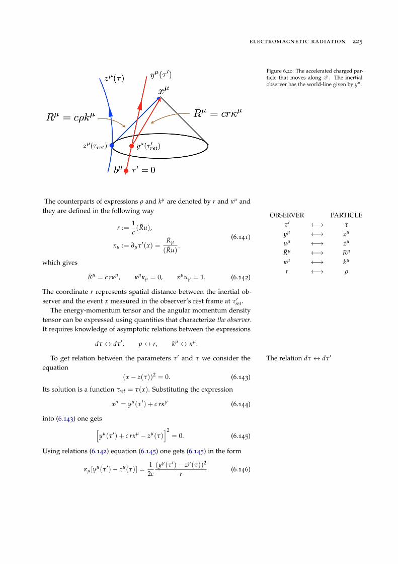
Figure 6.20: The accelerated charged par-ticle that moves along zµ. The inertialobserver has the world-line given by yµ.
The counterparts of expressions r and kµ are denoted by r and kµ and
OBSERVER PARTICLEt0 ! t
yµ ! zµ
uµ ! zµ
Rµ ! Rµ
kµ ! kµ
r ! r
they are defined in the following way
r :=1c(Ru),
kµ := ∂µt0(x) =Rµ
(Ru).
(6.141)
which gives
Rµ = c rkµ, kµkµ = 0, kµuµ = 1. (6.142)
The coordinate r represents spatial distance between the inertial ob-server and the event x measured in the observer’s rest frame at t0ret.
The energy-momentum tensor and the angular momentum densitytensor can be expressed using quantities that characterize the observer.It requires knowledge of asymptotic relations between the expressions
dt $ dt0, r$ r, kµ$ kµ.
To get relation between the parameters t0 and t we consider the The relation dt $ dt0
equation(x� z(t))2 = 0. (6.143)
Its solution is a function tret = t(x). Substituting the expression
xµ = yµ(t0) + c rkµ (6.144)
into (6.143) one getshyµ(t0) + c rkµ
� zµ(t)i2
= 0. (6.145)
Using relations (6.142) equation (6.145) one gets (6.145) in the form
kµ[yµ(t0)� zµ(t)] =12c
(yµ(t0)� zµ(t))2
r. (6.146)
226 lecture notes on classical electrodynamics
The right hand side of (6.146) vanishes at spatial infinity, r ! •, hence
kµ
⇣yµ(t0)� zµ(t)
⌘= O(r�1). (6.147)
which can be solved with respect to t giving some function Solution: t = t(t0, kµ)
t = t(t0, kµ) (6.148)
Let us consider the limit case for which the right hand side of (6.147)vanishes. Substituting (6.139) into (6.147) and using kµuµ = 1 one gets
t0 + kµbµ� kµzµ(t) = 0. (6.149)
The equation (6.149) implies the relation between differentials dt anddt0, namely
dt0 = (kz)dt. (6.150)
The relation r$ rThe relation between r and r can be deduced from the expression
xµ zµ(t), where xµ is expressed in two ways – involving world-line ofthe observer and world-line of the particle
[zµ(t) + c rkµ]zµ(t) = [yµ(t0) + c rkµ]zµ(t)
where kµ zµ(t) = 1. Solving with respect to r we get
r = kµ zµ(t) r +1c
⇣yµ(t0)� zµ(t)
⌘zµ.
Hence, r(r) = (kz) r + r0, where r0 is a term which does not depend onr. At spatial infinity dominates the first what gives asymptotic relation
r = (kz)r. (6.151)
The relation kµ $ kµ
Let us consider the expression xµ written in two different ways
zµ(t) + c rkµ = yµ(t0) + c rkµ. (6.152)
where t and t0 are related by t = t(t0, kµ). The inverse of t for theasymptotic case is given by (6.149). Contracting both sides of (6.152)with the light-like four-vector kµ one gets
kµkµ =
⇣yµ(t0)� zµ(t)
⌘kµ
cr.
According to (6.146) and (6.151) the expression kµkµ behaves at spatialinfinity as
kµkµ = O(r�2). (6.153)
electromagnetic radiation 227
The four-vector kµ derived from the equality (6.152) reads
kµ =rr
kµ +yµ(t0)� zµ(t)
cr.
It has the following dominant behaviour at spatial infinity
kµ =kµ
(kz)+O(r�1). (6.154)
Using the relations (6.150), (6.151) and (6.154) we get asymptotic Asymptotic form of tensors Tµnret
and Mµnaret at spatial infinityform of the tensors Tµn
ret and Mµnaret expressed in terms of quantities
associated withe the observer’s reference frame S0. Thus the leadingterm of the energy-momentum tensor reads
Tµnret = �
q2
4pc21
r2(kz)4
z2 + c2 (kz)2
(kz)4
�kµkn +O(r�3). (6.155)
For the angular momentum tensor we get
Mµnaret = zµTna
ret � znTµaret
+q2
4p
1r2(kz)4
kµ✓
zn�
(kz)(kz)
zn◆� kn
✓zµ�
(kz)(kz)
zµ◆�
ka+
+O(r�3) (6.156)
where
z ⌘dzdt
���t=t(t0 ,k)
and z ⌘d2zdt2
���t=t(t0 ,k)
.
The amount of four-momentum and angular momentum emitted bythe charged particle into the solid angle dW in the interval of time dt0
at the reference frame S0 read Tensors dPµ and dMµn are takenat spatial infinity
dPµ = limr!•
1c
Tµnret d3Sn, (6.157)
dMµn = limr!•
1c
Mµnaret d3Sa (6.158)
where d3Sµ is the spherical area element, r = const.We shall integrate expressions (6.157) and (6.158) choosing d3Sµ
as the area element on three-surface r = const. It is parametrizedby coordinates (ct0, J, j). The three-area element is obtained fromequation defining the three-surface r = r(xµ).
In what follows we consider a generic case of three-area elementd3Sµ associated with the surface obtained by fixing the value of one of The three-area element d3Sµ
four coordinates. Thus, we consider the diffeomorphism
zµ = zµ(xn), µ, n = 0, 1, 2, 3
where {xn} are Cartesian coordinates and {zµ} are curvilinear coordi-nates. The volume element d4W is given by dz4 ⌘ dz0dz1dz2dz3
228 lecture notes on classical electrodynamics
d4W =14!
eµnab∂(xµxnxaxb)
∂(z0z1z2z3)d4z
= eµnab∂xµ
∂z0∂xn
∂z1∂xa
∂z2∂xb
∂z3 d4z
= det✓
∂xr
∂zs
◆d4z =
q�g(z) d4z (6.159)
where d4z ⌘ dz0dz1dz2dz3 and g(z) ⌘ det�
g(z)�. On the other hand,
the four-volume element can be cast in the form dz3 ⌘ dz1dz2dz3
d4W =
✓∂xµ
∂z0 dz0◆✓
eµnab∂xn
∂z1∂xa
∂z2∂xb
∂z3 d3z
◆
=
✓∂xµ
∂z0 dz0◆✓
13!
eµnab∂(xnxaxb)
∂(z1z2z3)d3z
◆
=
✓∂xµ
∂z0 dz0◆
d3Sµ. (6.160)
Comparing (6.159) and (6.160) one gets
∂xµ
∂z0 d3Sµ =q�g(z) d3z
which can be cast in the form17 17 We apply the formula
∂xµ
∂zb
∂za
∂xµ = dab
for a = b = 0.
∂xµ
∂z0
d3Sµ �
∂z0
∂xµ
q�g(z) d3z
�= 0.
It gives
d3Sµ =∂z0
∂xµ
q�g(z) d3z. (6.161)
Now we go back to the particular case of spherical coordinates. Wechoose The case of the surface r = const
in spherical coordinatesz0 ⌘ r,
q�g(z)d3z = r2 sin J dJdj(cdt0).
The expression (6.161) gives dW ⌘ sin J dJdj
d3Sµ = (∂µr) r2(c dt0)dW. (6.162)
Taking derivative of (6.144) with respect to xµ and contraction of theobtained result with uµ we get
∂µxa = ua∂µt0(x) + c(∂µr) ka.
Henceda
µ = uakµ + cka∂µr.
Then, contracting this expression with ua, where kaua = 1, we getuµ = c2kµ + c∂µr. It gives
∂µr =uµ
c� c kµ. (6.163)
electromagnetic radiation 229
Note that ∂µr is a space-like vector that satisfies
(∂µr)(∂µr) =u2
c2 � 2(ku) + c2k2 = �1.
The element d3Sµ associated wit the surface r = const takes the form
d3Sµ =⇣
uµ � c2kµ
⌘r2dt0dW (6.164)
The four-momentum dPµ that crosses the area element r2dW of the Asymptotic form of quantitiesdPµ and dMµnsurface r = const during the time interval dt0 has asymptotic value
dPµ = limr!•
1c
Tµnret d3Sn = lim
r!•
1c
Tµnret (un � c2kn) dt0r2dW
= �q2
4pc31
r2(kz)4
z2 + c2 (kz)2
(kz)4
�kµkn(un � c2kn) dt0r2dW
= �q2
4pc31
(kz)4
z2 + c2 (kz)2
(kz)4
�kµdt0dW. (6.165)
The term Tµnret kn vanishes in the lowest orders, Tµn
ret kn µ r�4, becauseTµn
ret given by (6.155) is only asymptotic form of the energy momentumtensor. Indeed, according to (6.133) the retarded tensor Tµn
ret behaves atspatial infinity as ⇠ r�2kµkn, where r = (kz)r. Since knkn µ r�2 thenTµn
ret kn ⇠ r�4. Its contribution can be discarded because the integral ofthis quantity involving the element r2dW vanishes for r ! •.
Similarly, the asymptotic expression for the angular momentum isgiven by (6.156) and (6.164)
dMµn = limr!•
1c
Mµnaret d3Sa = lim
r!•
1c
Mµnaret (ua � c2ka) r2dt0dW
= zµdPn� zndPµ
+q2
4pc1
r2(kz)4
hkµ✓
zn�
(kz)(kz)
zn◆�
� kn✓
zµ�
(kz)(kz)
zµ◆ i
ka(ua � c2ka)dt0r2dW
= zµdPn� zndPµ
+q2
4pc1
(kz)4
kµ✓
zn�
(kz)(kz)
zn◆� kn
✓zµ�
(kz)(kz)
zµ◆�
dt0dW.
(6.166)
Integrating the expressions (6.165) and (6.166) over angles J andj we get total amount of four-momentum and angular momentum Integration over anglescarried by radiation. These integrals are evaluated in instantaneous restframe of the particle. In this reference frame, the observer’s four-velocitycoincide with particle’s four-velocity. The same is true for zaka anduaka = 1. Thus
(uk) = 1 = (zk), dt0 = dt. (6.167)
230 lecture notes on classical electrodynamics
There are three different types of integrals over angles
Iµ :=1
4p
Ikµ dW,
Iµn :=1
4p
Ikµkn dW,
Iµna :=1
4p
Ikµknka dW.
(6.168)
The formula (6.167) implies that
Iµuµ = 1, Iµnun = Iµ, Iµnaua = Iµn. (6.169)
The condition kµkµ = 0 implies
Iµnhµn = 0, Iµnahµn = Iµnahµa = Iµnahna = 0. (6.170)
The integrals (6.168) can be represented by combinations of symmetricexpressions build of the four-vector uµ and the metric tensor hµn. Themost general such combinations read
Iµ = auµ, (6.171)
Iµn = b1uµun + b2hµn (6.172)
Iµna = g1uµunua + g2⇥hµnua + haµun + hnauµ
⇤(6.173)
where free constants can be determined from identities (6.169).The first integral (6.171) contracted with uµ gives Iµuµ = 1 = ac2.
Thus a = 1c2 . The expression Iµnun = Iµ reduces to the equation
c2b1 + b2 = 1c2 . The second and independent equation follows from the
first relation (6.170), namely hµn Iµn = 0 = c2b1 + 4b2. These equationhave solution
b1 =4
3c4 , b2 = �1
3c2 .
Finally, the expression (6.173) takes the form
Iµnaua = c2g1uµun + g2[c2hµn + 2uµun]
=hc2g1 + 2g2
i
| {z }b1
uµun + c2g2|{z}b2
hµn.
It gives
g1 =2c6 , g2 = �
13c4 .
Substituting these results into (6.171) and (6.173) one gets Integrals (6.171) and (6.173)
Iµ =1c2 uµ, Iµn =
13c4
h4uµun � c2hµn
i, (6.174)
Iµna =1c6
"2uµunua �
c2
3(hµnua + hnauµ + haµun)
#. (6.175)

electromagnetic radiation 231
The result of integration of the expression (6.165) over angles has theform I
dPµ =⇣dPµ
dt
⌘dt
where18 18 Note that uµ ! zµ.
dPµ
dt= �
q2
4pc3
I hz2 + c2(kz)2
ikµdW
= �q2
c3
hz2 Iµ + c2 Iµna zn za
i. (6.176)
Substituting into (6.176) the integral Iµ = 1c2 zµ and the expression
Iµna zn za =1c6
"2
0z }| {zµ(zn zn)(za za)�
c2
3(hµn za + haµ zn + hna zµ)zn za
#
= �1
3c4 z2zµ,
where za za = 0, one gets The total four-momentum perunit of time carried by the radia-tion (it has dimension of force)dPµ
dt= �
2q2
3c5 z2zµ. (6.177)
Similarly, integrating the expression (6.166) over angles one getsI
dMµn =⇣dMµn
dt
⌘dt
where
dMµn
dt= zµ dPn
dt� zn dPµ
dt+
+q2
4pc
I hkµ�zn
� (kz)zn�� kn�zµ
� (kz)zµ�idW
= zµ dPn
dt� zn dPµ
dt+
+q2
c
hIµ zn� In zµ
��
Iµa zn za � Ina zµ za�i
| {z }Wµn
. (6.178)
The expression Wµn reads
Wµn =1c2�zµ zn
� zn zµ��
�1
3c4
h4
0z }| {�zµ za zn za � zn za zµ za
��c2�hµa zn za � hna zµ za
�i
=1c2 (z
µ zn� zn zµ)�
13c2 (z
µ zn� zn zµ)
=2
3c2 (zµ zn� zn zµ). (6.179)
232 lecture notes on classical electrodynamics
The angular four-momentum per unit of time carried out by radiationreads The total angular four-
momentum per unit of timecarried by radiation
dMµn
dt= zµ dPn
dt� zn dPµ
dt+
2q2
3c3
⇣zµ zn
� zn zµ⌘
(6.180)
This quantity has physical dimension of torque.
The Lorentz-Dirac equation
A charged particle in the presence of an external electromagnetic fieldexperiences the four-force
f µ =qc
Fµn zn. (6.181)
The particle’s four-momentum id denoted by pµ and their angularfour-momentum reads
mµn := zµ pn� zn pµ. (6.182)
Neglecting electromagnetic radiation, one gets that the rate of changeof particle’s four-momentum is equal to the four-force (6.181). Similarly,the rate of change change of its angular four-momentum is equal to atorque associated with the external electromagnetic field
dpµ
dt= f µ, (6.183)
dmµn
dt= zµ f n
� zn f µ, (6.184)
wheredmµn
dt= zµ dpn
dt� zn dpn
dt, (6.185)
dzµ
dtpn�
dzn
dtpµ = 0. (6.186)
According to (6.185) and (6.186), the rate of change of angular four-momentum of the particle depends only on the rate of change ofparticle’s four-momentum if the braking radiation is not taken intoaccount.
The particle’s equation of motion must be modified when brakingradiation (Bremsstrahlung) is taken into account. To do it we postulatethat the particle experiences additional reaction four-force “� dPµ
dt ” andadditional reaction four-torque “� dMµn
dt ”. The reaction force and torqueare expressed in terms of total four-momentum and four-angular mo-mentum per unit of time carried out by radiation. Equations of motion(6.183) and (6.184) must be substituted by the following ones
dpµ
dt= f µ
�dPµ
dt, (6.187)
dmµn
dt= zµ f n
� zn f µ�
dMµn
dt. (6.188)
electromagnetic radiation 233
Substituting (6.177) into the right hand side of (6.187) one gets
dpµ
dt= f µ +
2q2
3c5 z2zµ. (6.189)
The relation between four-momentum of the particle and its four-velocity is obtained from (6.187) and (6.188). The expression dmµn
dt
on the left hand side of (6.188) cannot simplify to (6.186) (otherwise,there would be pµ µ zµ). Indeed, the equation (6.188) can be cast in theform
ddt
(zµ pn� zn pµ) = zn f µ
� zµ f n�
2q2
3c3 (zµ zn� zn zµ)
which gives
⇣ dzµ
dtpn�
dzn
dtpµ⌘=
= 0 from (6.187)z }| {
�
⇣zµ dpn
dt� zn dpµ
dt
⌘+ zµ
✓f n�
dPn
dt
◆� zn
✓f µ�
dPµ
dt
◆
�2q2
3c3 (zµ zn� zn zµ).
The last equation reads
zµ✓
pn +2q2
3c3 zn◆� zn
✓pµ +
2q2
3c3 zµ◆= 0. (6.190)
It has the solution The relation between four-momentum four-velocity andfour-acceleration of the particlepµ = mzµ
�2q2
3c3 zµ (6.191)
where the term mzµ is must be included because it is a solution inthe case of vanishing acceleration. Note that four momentum of acharged particle (6.191) depends on particle’s four-velocity and four-acceleration. Taking derivative with respect to t of both sides of (6.191)and substituting dpµ
dt from (6.187) one gets the Lorentz-Dirac equation The Lorentz-Dirac equation
mzµ�
2q2
3c3
✓...z µ +
1c2 z2zµ
◆=
qc
Fµn zn. (6.192)
This equation describes a process of braking the particle due to emissionof radiation. Its solutions concord with experimental data to someextend. There are some problems associated with this equation. One ofthem is the existence of third order derivative. It requires an additionalinitial condition (initial value of the acceleration). Another problem isthe existence of non-physical solutions (self-accelerating). For instance,in absence of external electromagnetic field f µ = 0 the ansatz z2 = �a2
gives the linear equation
mzµ�
2q2
3c3
✓...z µ�
a2
c2 zµ◆= 0.
Among solutions of this equations there exists also a pathologicalsolution. Such a solution can be eliminated requiring zµ ! 0 fort ! •.
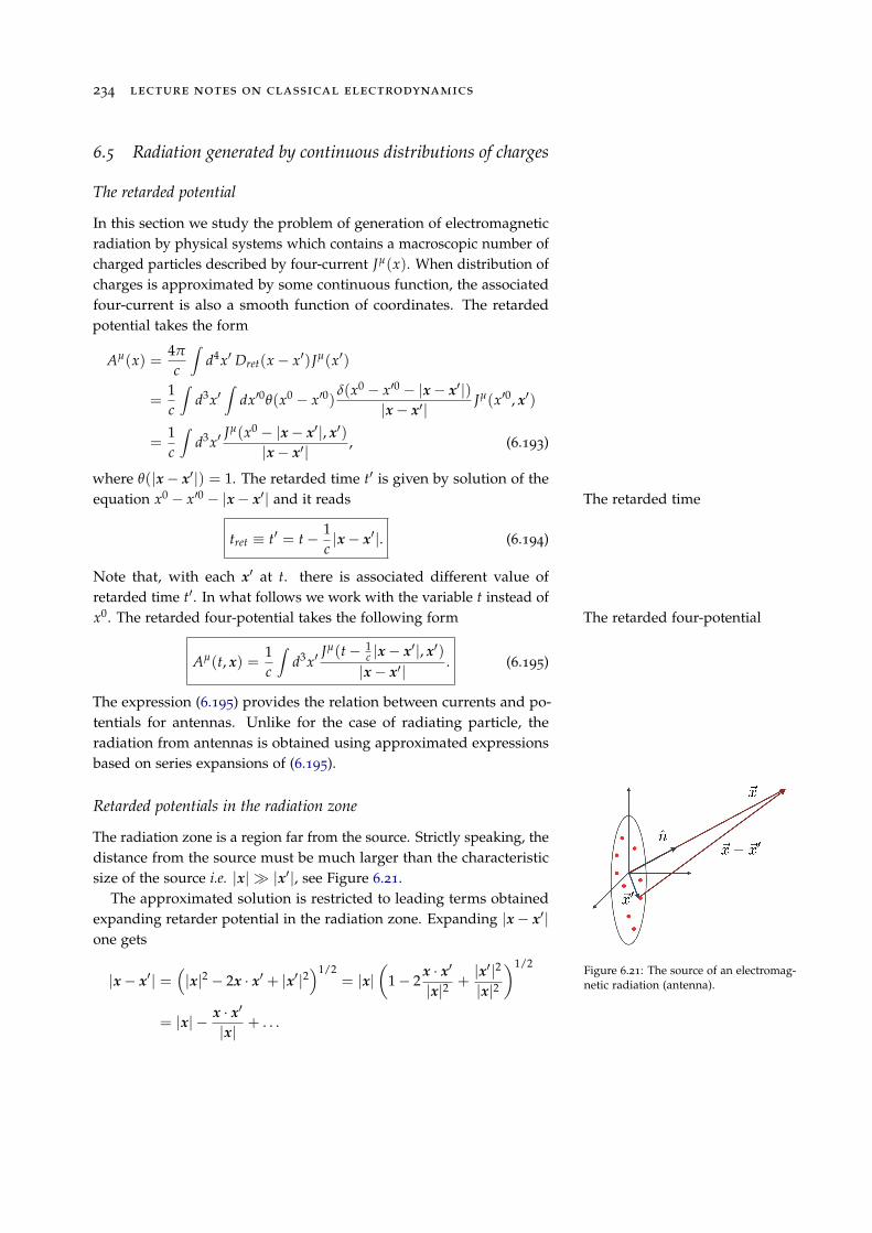
234 lecture notes on classical electrodynamics
6.5 Radiation generated by continuous distributions of charges
The retarded potential
In this section we study the problem of generation of electromagneticradiation by physical systems which contains a macroscopic number ofcharged particles described by four-current Jµ(x). When distribution ofcharges is approximated by some continuous function, the associatedfour-current is also a smooth function of coordinates. The retardedpotential takes the form
Aµ(x) =4p
c
Zd4x0 Dret(x� x0)Jµ(x0)
=1c
Zd3x0
Zdx00q(x0
� x00)d(x0 � x00 � |x� x
0|)|x� x0|
Jµ(x00, x0)
=1c
Zd3x0
Jµ(x0 � |x� x0|, x0)
|x� x0|, (6.193)
where q(|x� x0|) = 1. The retarded time t0 is given by solution of the
equation x0 � x00 � |x� x0| and it reads The retarded time
tret ⌘ t0 = t�1c|x� x
0|. (6.194)
Note that, with each x0 at t. there is associated different value of
retarded time t0. In what follows we work with the variable t instead ofx0. The retarded four-potential takes the following form The retarded four-potential
Aµ(t, x) =1c
Zd3x0
Jµ(t� 1c |x� x
0|, x0)
|x� x0|. (6.195)
The expression (6.195) provides the relation between currents and po-tentials for antennas. Unlike for the case of radiating particle, theradiation from antennas is obtained using approximated expressionsbased on series expansions of (6.195).
Retarded potentials in the radiation zone
The radiation zone is a region far from the source. Strictly speaking, thedistance from the source must be much larger than the characteristicsize of the source i.e. |x|� |x0|, see Figure 6.21.
Figure 6.21: The source of an electromag-netic radiation (antenna).
The approximated solution is restricted to leading terms obtainedexpanding retarder potential in the radiation zone. Expanding |x� x
0|
one gets
|x� x0| =
⇣|x|
2� 2x · x
0 + |x0|2⌘1/2
= |x|
✓1� 2
x · x0
|x|2+
|x0|2
|x|2
◆1/2
= |x|�x · x
0
|x|+ . . .
electromagnetic radiation 235
We denote r := |x| and n := x/|x|. It gives
|x� x0| = r� n · x
0 + . . . (6.196)
We shall restrict our consideration to first two terms of the expansion The retarded time
tret = t�rc+
1c
n · x0 + . . . where te := t�
rc
. (6.197)
We define emission time te as the retarded time of a source at the origin ofthe reference frame. By assumption, the origin of this frame is localizedinside the radiating region V. The expression te is the most roughapproximation for the retarded time. Thus, the term 1
c n · x0 represents
linear corrections to the retarded time associated with the finite size ofthe radiated system.
The partial derivatives of the retarded time with respect to spatialcoordinates xi read
∂itret = ∂i
✓t�
rc+
1c
n · x0 + . . .
◆
=1c
⇣�∂ir + ∂injx0j
⌘+ . . .
=1c
�ni +
dij � ninj
rx0j!+ . . .
=1c
✓�ni +
1r
⇣x0i � ni(n · x
0)⌘◆
+ . . .
=1c
✓�ni�
1r
hn⇥ (n⇥ x
0)ii◆+ . . .
which gives the gradient of tret The gradient of tret
rtret = �1c
✓n +
1r
n⇥ (n⇥ x0)
◆. (6.198)
The four-potential Aµ in the radiation zone is obtained expanding theexpression (6.195) and it reads
Aµ(t, x) =1c
Z
Vd3x0
Jµ(t� 1c (r� n · x
0 + . . .), x0)
r� n · x0 + . . .
=1c r
Z
Vd3x0(1 +
n · x0
r+ . . .)Jµ(te +
n · x0
c+ . . . , x
0)
=1c r
Z
Vd3x0
✓1 +
n · x0
r+ . . .
◆⇥
⇥
✓Jµ(te, x
0) +n · x
0
c∂t Jµ(te, x
0) + . . .◆
The region of integration is fixed (does not depend on time). Thus theintegral of partial derivative is equal to total derivative of the integral
Z
Vd3x ∂t f =
ddt
Z
Vd3x f .
236 lecture notes on classical electrodynamics
It gives The leading terms of the expan-sion
Aµ(t, x) =1c r
Z
Vd3x0 Jµ(te, x
0)+
+1
c2 rddt
Z
Vd3x0(n · x
0)Jµ(te, x0) + . . . (6.199)
We shall express the formula (6.199) in terms of dipole moments
p(t) :=1c
Zd3x0x0 J0(t, x
0), (6.200)
m(t) :=12c
Zd3x0x0 ⇥ J(t, x
0). (6.201)
The scalar potential is of the form
A0(t, x) =Qr+
1c r
n · p(te) + . . . (6.202)
where Q = const is the total electric charge of the configuration.The vector potential is obtained from (6.199), however, it requires
some work. First, we observe that the first integral (6.199) with µ =
{1, 2, 3} is equal to the time derivative of the electric dipole moment. Itcan be seen as follows. We take a closed surface S = ∂W which containsall the sources and has no common points or intersections with theregion V containing four-currents, V ⇢ W. It means that there are noelectromagnetic sources at the surface S i.e. Ji ⌘ 0 at S. Hence
I
S(x0i J j)daj = 0. (6.203)
The left hand side of this integral can be put in the form
I
S(x0i J j)daj =
Z
Wd3x0∂0j(x0i J j)
=Z
Vd3x0∂0j(x0i J j)
=Z
Vd3x0
hdij J j + x0i(∂0j J
j)i
=Z
Vd3x0 Ji
�
Z
Vd3x0 x0i∂tr
=Z
Vd3x0 Ji
�ddt
Z
Vd3x0 x0ir
=Z
Vd3x0 Ji
�dpi
dt
The integral (6.203) gives
Z
Vd3x0 J(te, x
0) = p(te). (6.204)
electromagnetic radiation 237
The second integral (6.199) can be transformed as follows
niZ
d3x0 x0i J j = ni 12
Zd3xh
x0i J j� x0j Ji
i+ ni 1
2
Zd3xh
x0i J j + x0j Jii
| {z }a quadrupole moment
= nic12c
Zd3xh
x0i J j� x0j Ji
i
| {z }eijkmk
+ · · ·
= �c[n⇥m]j + · · · (6.205)
The vector potential reads The vector potential
A(t, x) =1cr
[p(te)� n⇥ m(te)] + · · · (6.206)
where p(te) and m(te) are time derivatives of electric and magneticdipole moment.
Electric and magnetic field
Electric and magnetic fields are given by the four-potential components
E = �rA0�
1c
∂t A B = r⇥ A (6.207)
We shall skip all the terms which decrease faster than 1/r. Thus,expressions
r1r⇠
1r2
1rrni⇠
1r2 .
are not relevant. The electric field takes the form
E = �r
"Qr+
1c r
n · p(te)
#�
1c2r
hp(te)� n⇥ m(te)
i
= �1c r
(rte)| {z }�
n
c +···
n · p(te)�1
c2r
hp(te)� n⇥ m(te)
i+ · · ·
=1
c2 r
h(n · p)n� p| {z }
n⇥(n⇥p)
+n⇥ m
i+ · · ·
and thus
E =1
c2 rn⇥ [n⇥ p + m]
���te
(6.208)
The magnetic field reads
B = r⇥
1cr
hp(te)� n⇥ m(te)
i�
=1c r
(rte)| {z }�
n
c +...
⇥
hp(te)� n⇥ m(te)
i+ · · ·
238 lecture notes on classical electrodynamics
which gives
B =1
c2 rn⇥ [n⇥ m� p]
���te
(6.209)
The expressions (6.208) and (6.209) imply that B = n⇥ E.
Angular distribution of radiation
The radiated power is a function of angles. It can be cast in the form
dP(t) = (n · S)r2dW =c
4p|E|
2r2dW =c
4p|B|
2r2dW
=1
4pc3 [n⇥ [n⇥ p + m]]2dW
=1
4pc3 [[n⇥ p + m]2 � [n · (n⇥ p)| {z }
0
+n · m]2]dW
=1
4pc3 [(n⇥ p)2 + 2 (n⇥ p) · m| {z }
n·(p⇥m)
+ m2� (n · m)2
| {z }(n⇥m)2
]dW
which gives Angular distribution of thepower associated with the radia-tion fielddP(t) =
14pc3 [(n⇥ p)2 + (n⇥ m)2 + 2n · (p⇥ m)]
���te
. (6.210)
Integrating (6.210) over the angles one gets
P(t) =1
4pc3
" Z
V(n⇥ p)2dW +
Z
V(n⇥ m)2dW+
+ 2Z
Vn · (p⇥ m)dW
#. (6.211)
It is convenient to choose spherical coordinates independently for eachintegral (6.211). We choose these coordiantes in such a way that the zaxis is aligned with p in the first integral, with m in the second one andwith p⇥ m for third integral. It leads to expressions
Z(n⇥ p)2dW = 2p|p|
2Z p
0dJ sin3 J =
8p
3|p|
2, (6.212)Z(n⇥ m)2dW0 = 2p|m|
2Z p
0dJ0 sin3 J0 =
8p
3|m|
2, (6.213)Z
n · (p⇥ m)dW00 = 2p|p⇥ m|
Z p
0dJ00 sin J00 cos J00 = 0. (6.214)
The total radiated power calculated in the radiation zone reads The total pawer carried by radia-tion
P(t) =2
3c2
⇣|p|
2 + |m|2⌘
. (6.215)
Note, that |m|2 ⇠ c�2. It means that variation of magnetic dipolemoment contributes less than variation of electric dipole moment.
electromagnetic radiation 239
Taking for instance the electric charge q oscillating along the z axisone gets p = qz. Hence p = qz = qa.The total radiated power is givenby the Larmor formula
P(t) =2q2
3c3 a2. (6.216)
Related Documents