Lecture notes in KP8108 Advanced Thermodynamics Tore Haug-Warberg Department of Chemical Engineering NTNU (Norway) 23 February 2012 Exercise 1 Table of contents Exercise 153 Tore Haug-Warberg (ChemEng, NTNU) KP8108 Advanced Thermodynamics 23 February 2012 1 / 1598

Welcome message from author
This document is posted to help you gain knowledge. Please leave a comment to let me know what you think about it! Share it to your friends and learn new things together.
Transcript
Lecture notes
in
KP8108 Advanced Thermodynamics
Tore Haug-Warberg
Department of Chemical EngineeringNTNU (Norway)
23 February 2012
Exercise 1 Table of contents Exercise 153
Tore Haug-Warberg (ChemEng, NTNU) KP8108 Advanced Thermodynamics 23 February 2012 1 / 1598
−200 −160 −120 −800
100
200
300
400
500
600
700
800
900
Temperature [F]
Pre
ssur
e[p
sia]
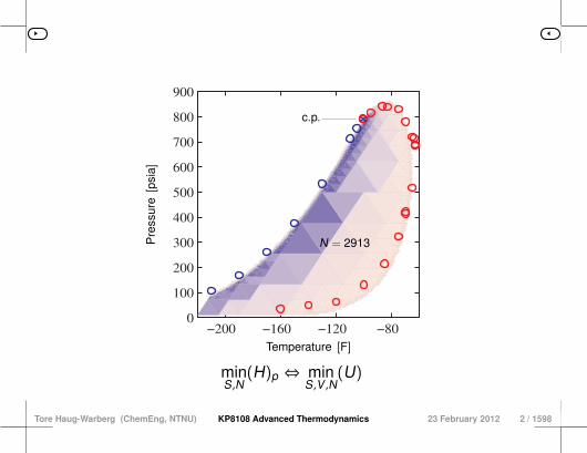
c.p.
N = 2913
minS,N
(H)p ⇔ minS,V ,N
(U)
Tore Haug-Warberg (ChemEng, NTNU) KP8108 Advanced Thermodynamics 23 February 2012 2 / 1598

Part-ContentsTitlepage . . . . . . . . . . . . . . . . . . . . . . . . . . . . . . . . . . . . . . . . . . . . . . . . . 1
1 List of symbols . . . . . . . . . . . . . . . . . . . . . . . . . . . . . . . . . . . . . . . . . . . . . . 6
2 Thermodynamic concepts . . . . . . . . . . . . . . . . . . . . . . . . . . . . . . . . . . . . . . . . 21
3 Prelude . . . . . . . . . . . . . . . . . . . . . . . . . . . . . . . . . . . . . . . . . . . . . . . . . . 54
4 The Legendre transform . . . . . . . . . . . . . . . . . . . . . . . . . . . . . . . . . . . . . . . . . 105
5 Euler’s Theorem on Homogeneous Functions . . . . . . . . . . . . . . . . . . . . . . . . . . . . . 167
6 Postulates and Definitions . . . . . . . . . . . . . . . . . . . . . . . . . . . . . . . . . . . . . . . . 221
7 Equations of state . . . . . . . . . . . . . . . . . . . . . . . . . . . . . . . . . . . . . . . . . . . . 239
8 State changes at constant composition . . . . . . . . . . . . . . . . . . . . . . . . . . . . . . . . . 340
9 Closed control volumes . . . . . . . . . . . . . . . . . . . . . . . . . . . . . . . . . . . . . . . . . 417
10 Dynamic systems . . . . . . . . . . . . . . . . . . . . . . . . . . . . . . . . . . . . . . . . . . . . 488
11 Open control volumes . . . . . . . . . . . . . . . . . . . . . . . . . . . . . . . . . . . . . . . . . . 532
Tore Haug-Warberg (ChemEng, NTNU) KP8108 Advanced Thermodynamics 23 February 2012 3 / 1598

Part-Contents (2)12 Gas dynamics . . . . . . . . . . . . . . . . . . . . . . . . . . . . . . . . . . . . . . . . . . . . . . 588
13 Departure Functions . . . . . . . . . . . . . . . . . . . . . . . . . . . . . . . . . . . . . . . . . . . 653
14 Simple vapour–liquid equilibrium . . . . . . . . . . . . . . . . . . . . . . . . . . . . . . . . . . . . 696
15 Multicomponent Phase Equilibrium . . . . . . . . . . . . . . . . . . . . . . . . . . . . . . . . . . . 746
16 Chemical equilibrium . . . . . . . . . . . . . . . . . . . . . . . . . . . . . . . . . . . . . . . . . . . 818
17 Simultaneous reactions . . . . . . . . . . . . . . . . . . . . . . . . . . . . . . . . . . . . . . . . . 869
18 Heat engines . . . . . . . . . . . . . . . . . . . . . . . . . . . . . . . . . . . . . . . . . . . . . . . 944
19 Entropy production and available work . . . . . . . . . . . . . . . . . . . . . . . . . . . . . . . . . 1011
20 Plug flow reactor . . . . . . . . . . . . . . . . . . . . . . . . . . . . . . . . . . . . . . . . . . . . . 1068
21 Material Stability . . . . . . . . . . . . . . . . . . . . . . . . . . . . . . . . . . . . . . . . . . . . . 1160
22 Thermofluids . . . . . . . . . . . . . . . . . . . . . . . . . . . . . . . . . . . . . . . . . . . . . . . 1214
24 T , s and p, v-Diagrams for Ideal Gas Cycles . . . . . . . . . . . . . . . . . . . . . . . . . . . . . . 1271
Tore Haug-Warberg (ChemEng, NTNU) KP8108 Advanced Thermodynamics 23 February 2012 4 / 1598
Part-Contents (3)25 SI units and Universal Constants . . . . . . . . . . . . . . . . . . . . . . . . . . . . . . . . . . . . 1279
26 Newton–Raphson iteration . . . . . . . . . . . . . . . . . . . . . . . . . . . . . . . . . . . . . . . 1295
27 Direct Substitution . . . . . . . . . . . . . . . . . . . . . . . . . . . . . . . . . . . . . . . . . . . . 1309
28 Linear Programming . . . . . . . . . . . . . . . . . . . . . . . . . . . . . . . . . . . . . . . . . . . 1318
29 Nine Concepts of Mathematics . . . . . . . . . . . . . . . . . . . . . . . . . . . . . . . . . . . . . 1337
30 Code Snippets . . . . . . . . . . . . . . . . . . . . . . . . . . . . . . . . . . . . . . . . . . . . . . 1355
Tore Haug-Warberg (ChemEng, NTNU) KP8108 Advanced Thermodynamics 23 February 2012 5 / 1598
Part 2
Thermodynamic concepts
see also Part-Contents
Tore Haug-Warberg (ChemEng, NTNU) KP8108 Advanced Thermodynamics 23 February 2012 21 / 1598

Contents
Tore Haug-Warberg (ChemEng, NTNU) KP8108 Advanced Thermodynamics 23 February 2012 22 / 1598
2 Thermodynamic . . .New issues
1 System
2 State
3 Process
4 Extensive vs. intensive
5 Equilibrium
6 Heat and work
Tore Haug-Warberg (ChemEng, NTNU) KP8108 Advanced Thermodynamics 23 February 2012 23 / 1598
2 Thermodynamic . . .ThermodynamicsThe language1 Language shapes our ability to think independently and to commu-
nicate and collaborate with other people.
2 It has enabled us to go far beyond simply meeting our basic needsassociated with survival and social interaction.
3 Our ability to observe, describe and record our thoughts aboutphysical phenomena is vital to a subject like thermodynamics.
4 For us it is particularly important to reach a common physical un-derstanding of abstract concepts such as energy and entropya, but aslanguages are always evolving, the premises for a shared conceptionare constantly shifting.
5 All authors have to contend with that dilemma, and few of us havethe good fortune to be writing for future generations.
6 The benefit of writing about a phenomenological subject such asthermodynamics is that as long as the observed phenomena remainunchanged, the subject will endure.
7 The challenge you face with a classical subject is combining thepreservation of an intellectual heritage with the injection of new ideas,and it is rather utopian to believe that the latter is possible in our case.
8 Since the rise of thermodynamics over the period 1840–1880, theoriginal beliefs have been replaced by a more (ope)rational interpreta-tion.
9 Meanwhile, the content has become so well-established and thor-oughly tested that there is little room for innovation, although there isstill scope to inject fresh life into old ideas.
24 / 1598
a As illustrated by Professor Gustav Lorentzen’s article: Bør Stortinget oppheve 2. hov-edsetning? (Should the Norwegian parliament abolish the second law of thermody-namics?), Ingeniør-nytt, 23(72), 1987 — written as a contribution to the debate on ther-mal power stations in Norway.
Notation1 Our understanding of thermodynamics depends on some vital, and
precisely defined, concepts that form part of a timeless vocabulary.
2 Accurate use of language improves our insight into the subject,thereby reducing the risk of misunderstandings.
3 However, an exaggerated emphasis on precision may overwhelmreaders and thus be counterproductive.
4 In this chapter we will revise and explain the key concepts in ther-modynamic analysisab in accurate, but nevertheless informal, terms.
5 Some of the concepts are concrete, whilst others are abstract, andit is by no means easy to understand them on a first read-through.
6 However, the aim is to convince readers that a good grasp of thebasic concepts is within reach, and that such a grasp is a prerequisitefor mastering the remaining chapters of the book.
25 / 1598
a James A. Beattie and Irwin Oppenheim. Principles of Thermodynamics. Elsevier,1979.b Rubin Battino, Laurence E. Strong, and Scott E. Wood. J. Chem. Eng. Educ.,74(3):304–305, mar 1997.
1 Thermodynamics describes natural phenomena in idealised terms.
2 The scope of the description can vary, and must be adapted to ourneeds at any given time.
6 3 The more details we want to understand, the more information wemust include in the description.4 The abstract concept of a “system” is at the heart of our under-
standing.5 A thermodynamic system simplifies physical reality into a mathe-
matical model. We can then use the model to perform thought experiments thatreveal certain characteristics of the system’s behaviour.7 Note that the physical size and shape of the system is quite irrele-
vant — all simple thermodynamic systems have uniform properties andcan always be described by a single set of state variables regardless ofthe actual geometry.8 That is an absolute principle.
Tore Haug-Warberg (ChemEng, NTNU) KP8108 Advanced Thermodynamics 23 February 2012 26 / 1598

2 Thermodynamic . . .§ 001 § 153 § 2
syste
mboundary
system
environment
Explain in your own words what is meant by the concepts:system, boundary and environment or surroundings.
Tore Haug-Warberg (ChemEng, NTNU) KP8108 Advanced Thermodynamics 23 February 2012 27 / 1598
2 Thermodynamic . . .§ 001 System
1 A system is a limited part of the universe with a boundary thatmay be a mathematical surface of zero thickness, or a physical barrierbetween it and the surroundings1.
2 A reservoir is a system that can interact with other systems withoutundergoing any change in its state variables. 3 Our physical surroundings such as the air, sea, lakes and bedrock
represent unlimited reservoirs for individual human beings, but not forthe entire world populationa.4 Similarly, a hydropower reservoir represents a thermodynamic
reservoir for the turbine, but not for the power company.5 This may appear trivial, but it is still worth trying to justify the above
statements to yourself or a fellow student.
a The first proof that the oceans were polluted by man came from Thor Heyerdahl’sRa II expedition in 1970. These reservoirs, and
other simple systems, have properties that are spatially and direction-ally uniform (the system is homogeneous with isotropic properties).
6 A real-world system will never be perfectly uniform, nor completelyunaffected by its surroundings, but it is nevertheless possible to makesome useful simplifying assumptions.7 Thus, a closed system, in contrast to an open one, is unable to
exchange matter with its surroundings.8 An isolated system can neither exchange matter nor energy.9 Note that the term control volume is used synonymously with open
system.10 The boundary is then called a control surface.11 In this context an adiabatic boundary is equivalent to a perfect in-sulator, and a diabatic boundary is equivalent to a perfect conductor.
1 We must be able to either actively control the system’s mass and composition, im-pulse (or volume) and energy, or passively observe and calculate the conserved quan-tities at all times. All transport properties ρ must satisfy limx→0+ ρ = limx→0− ρ so that ρis the same for the system and the surroundings across the control surface. In physics,this is called a continuum description. The exception to this is the abrupt change instate variables observed across a shock front. Well-known examples of this includehigh-explosive detonations and the instantaneous boiling of superheated liquids. It is
Tore Haug-Warberg (ChemEng, NTNU) KP8108 Advanced Thermodynamics 23 February 2012 28 / 1598

2 Thermodynamic . . .Properties
1 The state of a thermodynamic system is determined by the sys-tem’s properties — and vice versa.
3 2 The logic is circular, but experimentally the state is defined when allof the thermodynamic properties of the system have been measured. For example, the energy of the system is given by the formula
U = (∂U/∂X1)X1 + (∂U/∂X2)X2 + · · · once the state variables Xi andthe derived properties (∂U/∂Xi) are known.
6 4 This determines the value of U in one specific state.5 If we need to know the value of U in a number of different states, it
is more efficient to base our calculations on a mathematical model. (∂U/∂Xi) can then be calculated from the function U(X1,X2, . . .)
through partial differentiation with respect to Xi.
7 The measurements are no longer directly visible to us, but are in-stead encoded in the shape of model parameters (that describe the ob-servations to some degree at least).8 Normally it is only the first and secord derivatives of the model that
are relevant for our calculations, but the study of so-called critical pointsrequires derivatives up to the third or maybe even the fifth order.9 Such calculations put great demands on the physical foundation of
the model.
Tore Haug-Warberg (ChemEng, NTNU) KP8108 Advanced Thermodynamics 23 February 2012 29 / 1598
2 Thermodynamic . . .Variables
1 State variables only relate to the current state of the system.
2 In other words, they are independent of the path taken by the sys-tem to reach that state.
7 3 The number of state variables may vary, but for each (independent)interaction that exists between the system and its surroundings theremust be one associated state variable.4 In the simplest case, there are C + 2 such variables, where C is
the number of independent chemical components and the number 2represents temperature and pressure.5 The situation determines the number of chemical composition vari-
ables required.6 For example, natural fresh water can be described using C = 1
component (gross chemical formula H2O) in a normal steam boiler, orusing C = 5 components involving 9 chemical compounds in an isotopeenrichment planta.
a Naturally occurring water consists of a chemical equilibrium mixture of 1 H 1 H 16 O+2 H 2 H 16 O = 2(1 H 2 H 16 O) and others, formed by the isotopes 1 H, 2 H, 16 O, 17 O
and 18 O. The state of the system can be changed through what we call aprocess.
8 Terms such as isothermal, isobaric, isochoric, isentropic, isen-thalpic, isopiestic and isotonic are often used to describe simple physi-cal processes.
Tore Haug-Warberg (ChemEng, NTNU) KP8108 Advanced Thermodynamics 23 February 2012 30 / 1598
2 Thermodynamic . . .Variables (2)
9 Without considering how to bring about these changes in prac-tice, the terms refer to various state variables that are kept constant,such that the state change takes place at constant temperature, pres-sure, volume, entropy, enthalpy, (vapour) pressure or osmotic pressurerespectively.10 Generically the lines that describe all of these processes are some-
times called isopleths.11 Another generic expression, used in situations where the proper-ties of ideal gases are of prime importance (aerodynamics, combus-tion, detonation, and compression) is the polytropic equation of statep2/p1 = (V1/V2)γ.12 Here γ ∈ R can take values such as 0, 1 and cp/cv , which respec-tively describe the isobaric, isothermal and isentropic transformation ofthe gas.
Tore Haug-Warberg (ChemEng, NTNU) KP8108 Advanced Thermodynamics 23 February 2012 31 / 1598
2 Thermodynamic . . .§ 002 § 1 § 3
Explain in your own words what is meant by the terms:state, property, process and path.
Tore Haug-Warberg (ChemEng, NTNU) KP8108 Advanced Thermodynamics 23 February 2012 32 / 1598

2 Thermodynamic . . .§ 002 The state concept
1 A thermodynamic state is only fully defined once all of the relevantthermodynamic properties are known.
3 2 In this context, a thermodynamic property is synonymous with astate variable that is independent of the path taken by the systema.
a In simple systems, viscosity, conductivity and diffusivity also depend on the currentthermodynamic state, in contrast to rheology, which describes the flow properties of asystem with memory. Two examples of the latter are the plastic deformation of metalsand the viscosity of paint and other thixotropic liquids. In simple systems, the properties are (by definition) independent of
location and direction, but correctly identifying the system’s state vari-ables is nevertheless one of the main challenges in thermodynamics.
9 4 One aid in revealing the properties of the system is the process,which is used to describe the change that takes place along a givenpath from one state to another.5 In this context, a path is a complete description of the history of the
process, or of the sequence of state changes, if you like.6 Thermodynamic changes always take time and the paths are there-
fore time-dependent, but for a steady (flow) process the time is unim-portant and the path is reduced to a static state description of the inputand output states.7 The same simplification applies to a process that has unlimited time
at its disposal.8 The final state is then the equilibrium state, which is what is of
prime concern in thermodynamic analysis.
y
x
A cycle is the same as a closed path. The cycle can either betemporal (a periodic process) or spatial (a cyclic process). 10 This choice greatly affects the system description. In a steadystate, the variables do not change with time, whereas in dynamic sys-tems they change over time. Between these two extremes you have aquasi-static state: the state changes as a function of time, but in such away that the system is at all times in thermodynamic equilibrium, as de-scribed in greater detail in Paragraph 4.
Tore Haug-Warberg (ChemEng, NTNU) KP8108 Advanced Thermodynamics 23 February 2012 33 / 1598
2 Thermodynamic . . .§ 002 The state concept (2)
11 A state that is in thermodynamic equilibrium appears static at themacroscopic level, because we only observe the average properties ofa large number of particles, but it is nontheless dynamic at the molecu-lar level.
14 12 This means that we must reformulate the equilibrium principlewhen the system is small, i.e. when the number of particles n→ 0.13 At this extreme, intensive properties such as temperature, pressureand chemical potential will become statistical variables with some de-gree of uncertainty.
1±ε kg
1 kg+
−
In a theoretical reversible process, it is possible to reverse anychange of state by making a small change to the system’s interactionwith its surroundings.
17 15 Thus, two equal weights connected by a string running over a fric-tionless pulley will undergo a reversible change of state if the surround-ings add an infinitely small mass to one of the weights.16 This is an idealised model that does not apply in practice to anirreversible system, where a finite force will be required to reverse theprocess. Let us assume, for example, that the movement creates friction in
the pulley. You will then need a small, but measurable, change in massin order to set the weights in motion one way or the other.
Tore Haug-Warberg (ChemEng, NTNU) KP8108 Advanced Thermodynamics 23 February 2012 34 / 1598
2 Thermodynamic . . .§ 002 The state concept (3)
18 The total energy of the system is conserved, but the mechanicalenergy is converted into internal (thermal) energy in the process — so itis irreversible.19 If the friction is suddenly eliminated the weights will accelerate.
20 This change is neither reversible nor irreversible.21 Instead, it is referred to as lossless, which means that the mechan-ical energy is conserved without it necessarily being possible to reversethe process.22 For that to happen, the direction of the gravitational field would alsoneed to be reversed.
Tore Haug-Warberg (ChemEng, NTNU) KP8108 Advanced Thermodynamics 23 February 2012 35 / 1598

2 Thermodynamic . . .Extensive / intensive
1 2 In thermodynamics there are usually many (N > 2) state variables,as well as an infinite number of derived properties (partial derivatives). Experimentally it has been shown that the size of a system is pro-
portional to some of its properties. These are called extensive proper-ties, and include volume, mass, energy, entropy, etc.
3 Intensive properties, meanwhile, are independent of the size of thesystem, and include temperature, pressure and chemical potential.
8 4 Mathematically these properties are defined by Euler functions ofthe 1st and 0th degree respectively, as described in the separate chap-ter on the topic.5 There are also properties that behave differently.6 For example, if you increase the radius of a sphere, its surface area
and volume increase by r2 and r3 respectively.7 This contrasts with the circumference, which increases linearly with
the radius (it is extensive), and the ratio between the circumference andthe radius, which always remains 2π (it is intensive). The system’s mass is a fundamental quantity, which is closely re-
lated to inertia, acceleration and energy. An alternative way of measur-ing mass is by looking at the number of moles of the various chemicalcompounds that make up the system.
12 9 A mol is defined as the number of atomsa which constitute exactly0.012 kg of the carbon isotope 12 C, generally known as the Avogadroconstant NA = 6.022136(7)1023.10 In this context, molality and molarity are two measures of concen-tration stated in moles per kilogramme of solvent and moles per litre ofsolution respectively.11 These measures are not of fundamental importance to thermody-namics, but they are important concepts in physical chemistry, and aresometimes used in thermodynamic modelling.
a A mole is defined in terms of the prototype kilogramme in Paris and not vice-versa.Atomic mass is measured in atomic mass units, where the mass of one atom of the12 C isotope is defined as 12 amu. The 1 amu was originally defined as being equalin mass to one hydrogen atom, which deviates a little from the current definition. Thedeviation is due to a difference in nuclear energy between the two nuclei and is relatedto Einstein’s relation E = ∆mc2. Systems of variable mass contain a minimum number of indepen-
dent components that together make up the chemical composition ofthe system.
Tore Haug-Warberg (ChemEng, NTNU) KP8108 Advanced Thermodynamics 23 February 2012 36 / 1598

2 Thermodynamic . . .Extensive / intensive (2)
14 13 A component should here be considered a degree of freedom inGibbs’ phase rule F = C+2−P, where C is the number of componentsand P is the number of phases at equilibrium (see Paragraph 4). Only the composition at equilibrium can be described in these sim-
ple terms, which is because we are forced to specify as few as possiblevariables that depend on mass or the number of moles.15 This restriction influences our choice of components, and in prac-
tice the question is whether chemical reactions are taking place in thesystem, although the conventions of the applied discipline are equallyimportant.16 Generally components are selected from the system’s chemicalconstituents or species, or from its reactants, whereas for electrolytesand salt mixtures it is natural to use the ions that make up the system’schemical composition as componentsa.
a Components do not necessarily represent physical constituents. One example isternary recipocral systems (salt mixtures) of the type NaCl+KBr = NaBr+KCl, whichhave 4 possible substances (salts), but only 3 independent components. For example,the salt NaCl can be described by the vector (1,0,0,0), or (0,−1,1,1), or any linearcombination of these two vectors. This illustrates the use of a seemingly non-physical(in this case negative) number of moles for one of the components. The specificationdoes make sense, however, because the true amounts of each of the ions in themixture are non-negative, and hence real physical quantitites.
Tore Haug-Warberg (ChemEng, NTNU) KP8108 Advanced Thermodynamics 23 February 2012 37 / 1598
2 Thermodynamic . . .§ 003 § 2 § 4
Explain in your own words what is meant by a propertybeing intensive or extensive. If you divide an extensiveproperty by the number of moles in the system or its
mass, you get a molar or specific property respectively.Show that the property obtained is intensive.
Tore Haug-Warberg (ChemEng, NTNU) KP8108 Advanced Thermodynamics 23 February 2012 38 / 1598

2 Thermodynamic . . .§ 003 Size
1 In thermodynamics, size is not only a measure of the volume of asystem, but also of any properties related to its mass.
3 2 This implies that two systems with identical state descriptions be-come a system of double the size when combined. Properties that can be doubled in this way, such as entropy S,
volume V and the number of moles N, are proportional to the size ofthe system, and are referred to as extensive variables.
10 4 This means that all of the extensive variables must be increased bythe same factor.5 You cannot simply double the volume while keeping the number of
moles constant — entropy, volume and the number of moles must all bedoubled together.6 At the same time, other derived extensive properties like energy,
total heat capacity, etc. are scaled the same amount.7 Another group of properties is not affected by any change in the
size of the system.8 These properties are referred to as intensivea properties.9 Well-known examples include temperature T , pressure p and
chemical potential µ.
a The vague definitions of extensive and intensive used here will later be replaced byones involving Euler’s homogeneous functions of the 1st and 0th degree respectively. Certain pairs of extensive and intensive variables combine to form
a product with a common unit (most commonly energy), and feature inimportant relationships such as U = TS − pV + µ1N1 + µ2N2 + · · · .
11 These pairs of T and S, p and V , and µi and Ni are called conjugatevariables.
Tore Haug-Warberg (ChemEng, NTNU) KP8108 Advanced Thermodynamics 23 February 2012 39 / 1598

2 Thermodynamic . . .§ 003 Size (2)
15 12 A mechanical analogy is the flow rate ρ~V (extensive) and the grav-itational potential g∆z (intensive) at a hydropower station.13 The power generated by the turbine can be written g∆zρ~V , whichis the product of an intensive and extensive variable.14 Equivalent analogies can be found in electrical and mechanical en-gineering. Dividing one extensive property by another gives you a new, in-
tensive variable that represents the ratio between the two properties. 16 Let e.g. f = ax and g = bx be two extensive properties expressedas functions of x.
Then ρ = f/g = a/b is independent of x, in other words ρ is intensive.17 These kinds of variables are widely used to describe systems in away that does not refer to their size, but many fields have different prac-tices, and it is often unclear whether the definition is being expressedon a mass or mole basis (which is the most common source of misun-derstanding).18 The difference between a specific and a molar quantity is that oneis expressed per kilogramme and the other per mole of the substance(or mixture).19 Common examples include specific and molar heat capacity, spe-cific and molar volume, etc.
Tore Haug-Warberg (ChemEng, NTNU) KP8108 Advanced Thermodynamics 23 February 2012 40 / 1598
2 Thermodynamic . . .Degrees of freedom
1 Let us consider a thermodynamic system that does not changewith time, which means that it must be in equilibrium.
8 2 This minimises the degrees of freedom we have to specify.3 At high temperature chemical equilibrium, for example, it is suffi-
cient to state the quantity of each of the atoms present.4 The distribution of the atoms amongst the substances in the mix-
ture is determined by the principle of equilibrium (see below) and thesystem’s equation of state.5 In the case of phase equilibria, the chemical substances are sim-
ilarly distributed across the system’s phase boundaries and it is suffi-cient to specify the total composition of the entire system.6 As a rule of thumb these problems are easy to specifiy, but they
do nevertheless require numerical solution by iteration which in manycases is a challenging task.7 If the system has no internal degrees of freedom in the form of
chemical reactions or phase transformations, the equilibrium state willbe determined by an ordinary (but multivariate) function, generally with-out iteration. The general principles of equilibrium mean that the energy of the
system will be minimised with respect to all the degrees of freedom thatform the basis for the system description.
10 9 Alternatively the entropy is maximised with respect to its systemvariables. The degrees of freedom are at all times controlled by the physical
nature of the system, and this determines which extremal principle toapply.11 The theorectical foundations for this topic are discussed in a later
chapter on Legendre transformations.
Tore Haug-Warberg (ChemEng, NTNU) KP8108 Advanced Thermodynamics 23 February 2012 41 / 1598

2 Thermodynamic . . .§ 004 § 3 § 5Kinetics1 True equilibrium does not assert itself instantaneously, and from
our perspective it is not possible to judge whether equilibrium can beattained, or whether the system has kinetic limitations that prevent this.
2 All that thermodynamics does is describe the state of the systemat equilibrium, and not how long the process takes.
3 To describe in detail how the system changes over time we needan understanding of kinetics and transport theory.
4 Kinetics is the study of forces and the motion of bodies, whilst reac-tion kinetics looks specifically at rates of chemical reactions and phasetransitions.
5 Transport theory is a concept taken from nonequilibrium thermody-namics that can be used to describe the changes that take place in asystem until it reaches equilibrium.
6 As a general rule, all transport problems must be formulated aspartial differential equations, whereas thermodynamic equilibrium prob-lems can always be expressed using algebraic equationsa.
7 This difference in mathematical treatment reflects the gradients inthe system.
8 If they are not significant, it is sufficient to determine one represen-tative value for each of the scalar fields of temperature, pressure andchemical potential.
9 This distinguishes a thermodynamic problem from a transportproblem, where the scalar fields must be determined simultaneouslythroughout the space.
42 / 1598
a This is the difference between distributed and lumped description.
syste
mboundary
environment
phase b’ndary
α
βγ
Explain in your own words the following terms associatedwith equilibrium and equilibrium states: phase, phaseboundary, aggregate state, equilibrium and stability.
Tore Haug-Warberg (ChemEng, NTNU) KP8108 Advanced Thermodynamics 23 February 2012 43 / 1598

2 Thermodynamic . . .§ 004 Equilibrium
12 A phase is defined as being a homogeneous, macroscopic subsys-
tem separated from the rest of the system by a phase boundary.3 It must be possible to separate a phase from other phases through
mechanical means alone.4 This is an important prerequisite.5 The system’s equilibrium phases are often designated by the Greek
letters α, β, γ, etc.6 The entropy density, energy density and mass density are con-
stant within the phases, but they vary discontinuously across the phaseboundaries.7 Temperature, pressure and chemical potential, meanwhile, are
constant throughout the entire system (assuming equilibrium).8 Spatially a phase can be discretely distributed across the available
volume, cf. fog particles in air and drops of fat in milk.9 If the whole system only consists of one phase, it is said to be
homogeneous.10 Otherwise, it is heterogenous.11 A phase is referred to as incompressible if the volume is dependenton the pressure, but in reality all phases are compressible to a greateror lesser extent (particularly gases).12 In principle a phase has two possible states of matter: crystallineand non-crystalline (glass and fluids).13 For practical purposes a fluid may sometimes be referred to asa gas without a specific volume, a liquid with surface tension, or anelectrically conductive plasma, but in thermodynamics there is a gradualtransition between these terms, and there are no strict criteria as to whatfalls within which category.
stable
metastable
unstable
Equilibrium is the state attained by the system when t →∞.
14 If the system returns to the same equilibrium state after exposureto a large random perturbation (disturbance), the equilibrium is said tobe stable.
15 A metastable equilibrium is stable when exposed to minor pertur-bations, but it becomes unstable in the event of major displacements.
19 16 An unstable equilibrium is a mathematical limit case.17 It describes a material state that breaks down if exposed to infinitelysmall perturbations.18 It is impossible to physically create this kind of equilibrium, but it isnevertheless very important from a theoretical point of view, as it sets alimit on what can physically exist based on simple laws of physics andmathematics. If the stability limit is exceeded, the system will split into two or
more equilibrium phases (from the mechanical analogy in the figure itis equally likely that the ball will fall to the right as to the left).
Tore Haug-Warberg (ChemEng, NTNU) KP8108 Advanced Thermodynamics 23 February 2012 44 / 1598

2 Thermodynamic . . .(In)exact differential Surroundings1 The assumptions and limitations set out in this chapter, and in thebook as a whole, in relation to thermodynamic system analysis, aresufficient for the purposes of analysing the effects of a large number ofchanges of state, but they do not tell us anything about how the systemrelates to its surroundings.
2 In order to analyse that, we must introduce two further terms,namely work W and heat Q .
3 These two properties control the system’s path as a function of itsphysical relationship to its surroundings.
4 On the one hand you have the abstract analysis of the system,which deals with state functions and mathematical formulae, and on theother you have an equally idealised interpretation of the surroundings.
5 Within this context, heat and work are defined as two differentmodes of exchanging energy.
6 It is important to note that heat and work are not state variablesof the system: they simply describe two different mechanisms for ex-changing energy between the system and its surroundings.
45 / 1598
1 State variables are variables that form part of a state function.
2 A state function always produces an exact differential, but not alldifferentials in physics are exact2.
3 One example from thermodynamics is (dU)n = δQ − δW , whichdescribes the energy balance for a closed system. Here the energy Uis a state function with the total differential (dU)n.
4 For any change δQ − δW there is a unique value of (dU)n.
6 5 However, the reverse is not true. For any change (dU)n there are in principle an infinite number ofcombinations of δQ and δW , since only the difference between heatand work is observable.
Tore Haug-Warberg (ChemEng, NTNU) KP8108 Advanced Thermodynamics 23 February 2012 46 / 1598

2 Thermodynamic . . .(In)exact differential (2)
2 Let e.g. f(x , y) = xy + c be a state function with x and y as its state variables. Heredf = y dx + x dy is the total differential of the function. The right side of the equationis then called exact. If as a pure thought experiment we change the plus operator onthe right side to minus, the differential becomes non-exact. It is possible to transformthe left-hand side into y2 dg = y δx − x δy, where y2 is an integrating factor for thedifferential and dg is the total differential of g(x , y) = xy -1 + c, but the new differentialy δx − x δy remains non-exact, since it cannot be expressed as the total differential ofany known function.
Tore Haug-Warberg (ChemEng, NTNU) KP8108 Advanced Thermodynamics 23 February 2012 47 / 1598

2 Thermodynamic . . .§ 005 § 4 § 6
δW
δQ
dU=δ
Q− δW
Explain in your own words the meaning of the terms:heat, work and energy. Are all three state variables?
Tore Haug-Warberg (ChemEng, NTNU) KP8108 Advanced Thermodynamics 23 February 2012 48 / 1598
2 Thermodynamic . . .§ 005 Heat and work
1 Heat and work are two closely related mechanisms for transportingenergy between the system and its surroundings.
2 Transporting energy affects the state of the system, but the heatand work are not themselves accumulated in the system.3 Work involves moving a macroscopic mass, or elementary parti-
cles, against an external force.4 A moving piston, a rotating axle, electrons in an electric circuit and
water flowing through a turbine are all examples of this.5 Heat results from large numbers of random, microscopic move-
ments that do not result in any net movement of mass.6 For heat to be converted into work, the microscopic movements
must first be coordinated.7 The 2nd law of thermodynamics then dictates that some of the heat
will be lost to a thermal reservoir of the same temperature as the sur-roundings.8 The term energy dissipation is used to emphasise the fact that
spontaneous processes always result in a reduction in available energy.9 The convention is for work done and heat supplied to be expressed
as positive values.10 Individually, neither heat nor work are state variables, but the differ-ence between them gives us the change in the system’s energy, whichis a state function.11 In other words, any given change in energy can be produced in aninfinite number of ways by varying the contributions made by heat andwork.
Tore Haug-Warberg (ChemEng, NTNU) KP8108 Advanced Thermodynamics 23 February 2012 49 / 1598
2 Thermodynamic . . .Das Ding an sich
1 2 Having defined the fundamental concepts, what we now must do isturn theory into practice.3 That will require a good understanding of the physics involved in
the problems that we will be looking at, some mathematics and in par-ticular differential equations and linear algebra, and a selection of rele-vant descriptions of substances, known as equations of state. Last but not least, we need to know the purpose of our analysis.
7 4 It is often based in a wish to find a simple model to explain thechanges in the system’s state.5 Thermodynamics is, in short, a subject that combines most of the
things taught in undergraduate chemistry, physics and mathematics atthe university.6 However, it is somewhat optimistic to believe that mechanical en-
gineering, thermodynamics, electromagnetism and other calculation-heavy subjects can fully describe the world we live in, and that we arein a position to decide how detailed an answer we want. Mathematics provides us with a useful tool, but that does not mean
that models and reality are two sides of the same coin, and hence thatwe, by carefully eliminating “all” assumptions, can reach an absolutelytrue answer.
8 Mathematical descriptions allow us to understand some character-istic events that surround us, but they do not give us the whole picture.
Tore Haug-Warberg (ChemEng, NTNU) KP8108 Advanced Thermodynamics 23 February 2012 50 / 1598

2 Thermodynamic . . .Das Ding an sich (2)
Duck or rabbit ?
9 Immanuel Kant3 unified the most im-portant strands of rationalism and empiri-cism with his interpretation of das Dingan sich. 10 He stressed that we can never be certain about the intrinsic, true
nature of anything, and that our understanding of the world is limited byour subjective experiences in time and space. Science is based on observable
events taking place in a world where timeand space are assumed to be indepen-dent of us, but from a philosophical pointof view Kant argues that we may be un-able to see all the aspects of whatever weare observing.
14 11 For example, does the picture on the left represent a duck or arabbit?12 With a bit of imagination we can spot both animals, but we can onlysee one of them at any given time.13 The full picture is not available to us, and at first glance we don’teven realise that there are two possibilitiesa.
b
b
b
bbb
b
b
b
32 J mol-1
h
x
∆rxh or ∆mıxh ?
⊗
⊗
⊗⊗
⊗ ⊗
⊗
⊗
⊗
bC bC bCbC bC bCbC bC bC
a At first glance, around half of the population will see the duck, whilst the other halfwill see the rabbit. Thermodynamics is really a subject that describes das Ding für
uns4 as opposed to das Ding an sich.
Tore Haug-Warberg (ChemEng, NTNU) KP8108 Advanced Thermodynamics 23 February 2012 51 / 1598

2 Thermodynamic . . .Das Ding an sich (3)
16 15 The figure on the right illustrates this distinction in a rather subtlemanner. The solid circles show calometric readings for the mixing enthalpy
∆mıxh of the system H2O–D2O5 at varying compositions (mole fractionsx) of the two compounds.
18 17 The continuous line has been fitted using the semi-empiric modelax(1 − x), which gives a first-order approximation of ∆mıxh. The line fits the data points very well, and we can therefore con-
clude that this simple model adequately represents the readings taken.
20 19 This posture is, in simple terms, what is meant by das Ding für uns. Based on our understanding of nature, isotopes are chemicallyidentical, but in this case the mixing enthalpy measured is equivalentto a fall in temperature of 0.43 K for an equimolar mixture of the twoisotopes, which is much greater than expected.
2721 The reason for this discrepancy is that the two components reactendothermically to form HDO.22 The net reaction involves the protonation of H2O⇔ H++OH− andthe deuteronation of D2O⇔ D++OD− which are fast reactions.23 The result is that H2O+D2O ⇔ 2 HDO reaches equilibriuma in avirtually ideal mixture.24 The last statement appears to be self-contradictory, as the compo-nents react chemically at the same time as they take part in an idealequilibrium.25 This apparent contradiction arises because of the unclear bound-ary between a chemical reaction and a physical interaction.26 For a thin gas there is an explanation for this, but for a liquid thereis no entirely satisfactory definition.
a In the system CD3OD–CH3OD, covalent bonds form between C–D and C–H, pre-venting any isotopic reaction, meaning that the change in enthalpy is only 0.79 J mol-1
or 0.01 K; cf. T. Kimura et al. J. Therm. Anal. Cal., 64:231–241, 2001, shown as opencircles in the figure. Subsituting OD to OH changes the chemistry to CD3OD–CH3OH
which again allows for proton–deuteron exchange and the equimolar change in en-thalpy increases to an intermediate value of 8.4 J mol-1 or 0.1 K. The reaction product HDO is not stable either since it decomposes
instantaneously to H2O and D2O, which prevents us from observingthe substance in its pure state.
Tore Haug-Warberg (ChemEng, NTNU) KP8108 Advanced Thermodynamics 23 February 2012 52 / 1598
2 Thermodynamic . . .Das Ding an sich (4)
29 28 Our understanding of nature is, in other words, based on evidencederived from indirect observations and mathematical models of thephysical properties in the water phase. In reality all scientific knowledge is based on theoretical models of
one kind or the other, and therefore does not imply that we have anyexact understanding of das Ding an sich.
30 The foundations of phenomenological thermodynamics are tooweak to state hard facts about the true nature of the systems it de-scribes, but strangely enough thermodynamic theory can still be usedto falsify claims that break the laws upon which it is founded6.
32 31 The theoretical basis is also sufficient for deriving important rela-tionships between the state variables, but it does not constitute inde-pendent evidence in the mathematical sense. Thermodynamic analysis is capable of confirming prior assump-
tions, or of demonstrating new relationships between existing results,but the calculations are not necessarily correct even if the model ap-pears to correspond with reality.
Tore Haug-Warberg (ChemEng, NTNU) KP8108 Advanced Thermodynamics 23 February 2012 53 / 1598

2 Thermodynamic . . .Das Ding an sich (5)
34 33 Firstly, the result is limited to the sample space for the analysisand to the underlying assumptions and secondly, there may be severalequally good explanations for a single phenomenon (as shown in theenthalpy example above). It is also worth remembering that even a small one-component
system has maybe 1015–1020 microscopic degrees of freedom that aremodelled with only three thermodynamic state variables7.
36 35 This means that a significant amount of information about the sys-tem is lost along the way. It is therefore necessary to develop our ability to recognise what
is important for the modelling, so that we can perform the right cal-culations, rather than trying to look (in vain) for the very accuratedescription.37 In keeping with that principle, we will mainly be looking at simple
models such as ideal gas and the van der Waals equation, but that doesmean that we will be very precise in our analysis of the ones that we dolook at.
3 Immanuel Kant, 1724–1804. German philosopher and logician.4 Referred to as Erscheinung in Kant’s thesis.5 D. V. Fenby and A. Chand. Aust. J. Chem., 31(2):241–245, 1978.6 The perpetuum mobile is the most famous example of this. In Norway it is in factimpossible to apply for patent protection for a perpetual motion machine, cf. the Nor-wegian Industrial Property Office’s Guidelines for processing patent applications. Theonline (2010) version of Part C: Preliminary examination; Chapter II Contents of thepatent application, except requirements; 3.3.6 Insufficient clarity excludes inventionsthat “. . . are inherently impossible to produce, as doing so would require acceptedphysical laws to be broken — this applies e.g. to perpetual motion machines.”7 Systems with many components are obviously even more complex.
Tore Haug-Warberg (ChemEng, NTNU) KP8108 Advanced Thermodynamics 23 February 2012 54 / 1598
2 Thermodynamic . . .Looking back
1 System
2 State
3 Process
4 Extensive vs. intensive
5 Equilibrium
6 Heat and work
Tore Haug-Warberg (ChemEng, NTNU) KP8108 Advanced Thermodynamics 23 February 2012 55 / 1598
Canonical potentials Manifolds Inversion Maxwell relations Gibbs–Helmholtz equation
Part 4
The Legendre transform
see also Part-Contents
Tore Haug-Warberg (ChemEng, NTNU) KP8108 Advanced Thermodynamics 23 February 2012 112 / 1598
Canonical potentials Manifolds Inversion Maxwell relations Gibbs–Helmholtz equation
Contents
1 Canonical potentials
2 Manifolds
3 Inversion
4 Maxwell relations
5 Gibbs–Helmholtz equation
Tore Haug-Warberg (ChemEng, NTNU) KP8108 Advanced Thermodynamics 23 February 2012 113 / 1598
Canonical potentials Manifolds Inversion Maxwell relations Gibbs–Helmholtz equation
4 The . . .Energy
1 2 The formal definition of the canonical thermodynamic potentials isone of the three fundamental pillars of thermodynamic theory,a togetherwith the principle of equilibrium, and the somewhat opaque distinctionbetween heat and work.bc.3 This is the background to what we will now discuss, but for the mo-
ment we will refrain from examining to what extent mathematical formu-lae are of practical relevance to the applications of the theory.4 Complications arise from the fact that there are several energy
functions to choose from, and it can be difficult to know exactly whichfunction is best suited for a particular problem.
a I.e. the functions U(S ,V ,N), H(S ,p,N), A(T ,V ,N), G(T ,p,N), etc.b Herbert Callen. Thermodynamics and an Introduction to Thermostatistics. Wiley, 2ndedition, 1985.c Michael Modell and Robert C. Reid. Thermodynamics and Its Applications. PrenticeHall, 2nd edition, 1983. From a pragmatic point of view it is convenient to remember that
U is useful for dynamic simulation, H for stationary simulation, etc. If afeasible solution to the problem already exists then this is perfectly ad-equate, but when seeking a new solution we need a deeper theoreticalunderstanding.
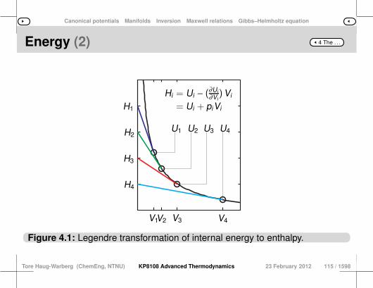
5 Here, the Legendre1 transformation is the key, as it provides asimple formula that allows us replace the free variable of a functionwith the corresponding partial derivative. For example, the variableV in internal energy U(S ,V ,N) can be replaced by (∂U/∂V)S,N , seeFigure 4.1.
Tore Haug-Warberg (ChemEng, NTNU) KP8108 Advanced Thermodynamics 23 February 2012 114 / 1598
Canonical potentials Manifolds Inversion Maxwell relations Gibbs–Helmholtz equation
4 The . . .Energy (2)
H1
H2
H3
H4
Hi = Ui − (∂Ui∂Vi
)Vi
= Ui + piVi
U1 U2 U3 U4
V1V2 V3 V4
Figure 4.1: Legendre transformation of internal energy to enthalpy.
Tore Haug-Warberg (ChemEng, NTNU) KP8108 Advanced Thermodynamics 23 February 2012 115 / 1598
Canonical potentials Manifolds Inversion Maxwell relations Gibbs–Helmholtz equation
4 The . . .Energy (3)
6 The new variable can be interpreted as the negative pressure π
and the resulting transformed function, called enthalpy H(S , π,N), is inmany cases more versatile than U itself. In fact, as we will see later, Hhas the same information content as U.7 This is one of the key reasons why the Legendre transformation is
central to both thermodynamic and mechanical theory.
1 Adrien-Marie Legendre, 1752–1833. French mathematician.
Tore Haug-Warberg (ChemEng, NTNU) KP8108 Advanced Thermodynamics 23 February 2012 116 / 1598
Canonical potentials Manifolds Inversion Maxwell relations Gibbs–Helmholtz equation
4 The . . .Transformation rules
1 Mathematically, the Legendre transformation φi of the function f isdefined by:
φi(ξi , xj , xk , . . . , xn) = f(xi , xj , xk , . . . , xn) − ξixi ,
ξi =( ∂f∂xi
)xj ,xk ,...,xn
. (4.1)
2 As mentioned above, one example of this is the transformation ofinternal energy to enthalpy:
H = UV (S , π,N) = U(S ,V ,N) − πV
π =(∂U∂V
)S,N = − p
Note that the volume derivative of U is the negative pressure π, becauseU diminishes when the system performs work on the surroundings —not vice versa.
Tore Haug-Warberg (ChemEng, NTNU) KP8108 Advanced Thermodynamics 23 February 2012 117 / 1598
Canonical potentials Manifolds Inversion Maxwell relations Gibbs–Helmholtz equation
4 The . . .Transformation rules (2)
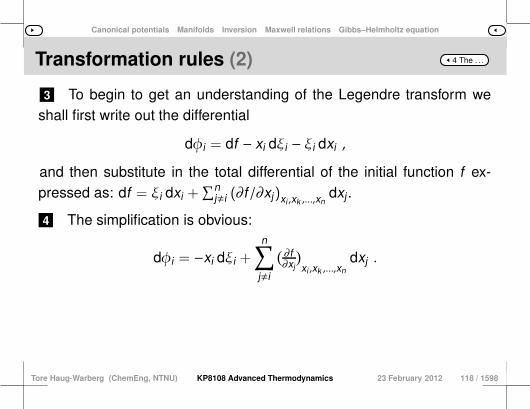
3 To begin to get an understanding of the Legendre transform weshall first write out the differential
dφi = df − xi dξi − ξi dxi ,
and then substitute in the total differential of the initial function f ex-pressed as: df = ξi dxi +
∑nj,i (∂f/∂xj)xi ,xk ,...,xn
dxj .
4 The simplification is obvious:
dφi = −xi dξi +
n∑
j,i
( ∂f∂xj
)xi ,xk ,...,xn
dxj .
Tore Haug-Warberg (ChemEng, NTNU) KP8108 Advanced Thermodynamics 23 February 2012 118 / 1598
Canonical potentials Manifolds Inversion Maxwell relations Gibbs–Helmholtz equation
4 The . . .Transformation rules (3)
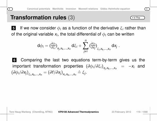
5 If we now consider φi as a function of the derivative ξi rather thanof the original variable xi, the total differential of φi can be written
dφi =(∂φi
∂ξi
)xj ,xk ,...,xn
dξi +
n∑
j,i
(∂φi
∂xj
)ξi ,xk ,...,xn
dxj .
6 Comparing the last two equations term-by-term gives us theimportant transformation properties (∂φi/∂ξi)xj ,xk ,...,xn
= −xi and(∂φi/∂xj)ξi ,xk ,...,xn
= (∂f/∂xj)xi ,xk ,...,xn= ξj .
Tore Haug-Warberg (ChemEng, NTNU) KP8108 Advanced Thermodynamics 23 February 2012 119 / 1598

Canonical potentials Manifolds Inversion Maxwell relations Gibbs–Helmholtz equation
4 The . . .Transformation rules (4)
7 The latter shows that further transformation is straightforward:
φij(ξi , ξj , xk , . . . , xn) =φi(ξi , xj , xk , . . . , xn) − ξjxj , (4.2)
ξj =(∂φi∂xj
)ξi ,xk ,...,xn
=( ∂f∂xj
)xi ,xk ,...,xn
.
Tore Haug-Warberg (ChemEng, NTNU) KP8108 Advanced Thermodynamics 23 February 2012 120 / 1598
Canonical potentials Manifolds Inversion Maxwell relations Gibbs–Helmholtz equation
4 The . . .Repeated transformation
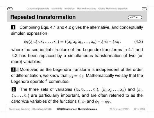
1 Combining Eqs. 4.1 and 4.2 gives the alternative, and conceptuallysimpler, expression
φij(ξi , ξj , xk , . . . , xn) = f(xi , xj , xk , . . . , xn) − ξixi − ξjxj , (4.3)
where the sequential structure of the Legendre transforms in 4.1 and4.2 has been replaced by a simultaneous transformation of two (ormore) variables.
5 2 The two alternative approaches are equivalent because ξj is thesame regardless of whether it is calculated as (∂φi/∂xj)ξi ,xk ,...,xn or as(∂f/∂xj)xi ,xk ,...,xn
3 This is clear from the differential equation above, and from Para-graph 20 on page 122.4 Knowing the initial function f and its derivatives is therefore suffi-
cient to define any Legendre transform. Moreover, as the Legendre transform is independent of the orderof differentiation, we know that φij = φji. Mathematically we say that theLegendre operator2 commutes.
6 The three sets of variables (xi , xj , . . . , xn), (ξi , xj , . . . , xn) and (ξi ,
ξj , . . . , xn) are particularly important, and are often referred to as thecanonical variables of the functions f , φi and φij = φji.
Tore Haug-Warberg (ChemEng, NTNU) KP8108 Advanced Thermodynamics 23 February 2012 121 / 1598
Canonical potentials Manifolds Inversion Maxwell relations Gibbs–Helmholtz equation
4 The . . .Repeated transformation (2)
2 Mathematical operators are often allocated their own symbols, but in thermodynamicsit is more usual to give the transformed property a new function symbol.
Tore Haug-Warberg (ChemEng, NTNU) KP8108 Advanced Thermodynamics 23 February 2012 122 / 1598

Canonical potentials Manifolds Inversion Maxwell relations Gibbs–Helmholtz equation
4 The . . .Canonical potentials
1 2 The legal system of the Roman Catholic Church, also called canonlaw, has medieval roots, and is based on a collection of texts that theChurch considers authoritative (the canon).3 Today the word canonical is used to refer to something that is or-
thodox or stated in a standard form.4 The latter definition is particularly used in mathematics, where e.g.
a polynomial written with the terms in order of descending powers issaid to be written in canonical form. In thermodynamics, we refer to canonical potentials, meaning
those that contain all of the thermodynamic information about the sys-tem.
5 Here we will show that the Legendre transforms of internal energygive us a canonical description of the thermodynamic state of a system.
6 Essentially, what we need to show is that U(S ,V ,n), A(T ,V ,n),H(S ,−p,n), etc. have the unique property that we can recreate all ofthe available information from any single one of them.
7 This is not trivial, as we will see that U(T ,V ,n) and H(T ,−p,n), forinstance, do not have this property.
Tore Haug-Warberg (ChemEng, NTNU) KP8108 Advanced Thermodynamics 23 February 2012 123 / 1598

Canonical potentials Manifolds Inversion Maxwell relations Gibbs–Helmholtz equation
4 The . . .§ 019 § 18 § 20
Derive all of the possible Legendre transforms ofinternal energy. State carefully the canonical variables
in each case. Use the definitions3 τ = (∂U/∂S)V ,N,π = (∂U/∂V)S,N and µ = (∂U/∂N)S,V to help you.
3 Let τ and π denote temperature and negative pressure respectively. This is to em-phasize that they are transformed quantities, like the chemical potential µ. In this no-tation, all intensive derivatives of internal energy are denoted by lower case Greek let-ters.
Tore Haug-Warberg (ChemEng, NTNU) KP8108 Advanced Thermodynamics 23 February 2012 124 / 1598
Canonical potentials Manifolds Inversion Maxwell relations Gibbs–Helmholtz equation
4 The . . .§ 019 Energy functions
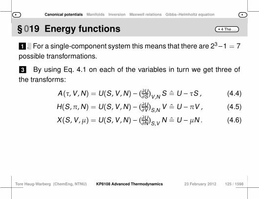
1 2 For any given thermodynamic function with m = dim(n) + 2 vari-ables there are 2m − 1 Legendre transforms. For a single-component system this means that there are 23−1 = 7
possible transformations.
3 By using Eq. 4.1 on each of the variables in turn we get three ofthe transforms:
A(τ,V ,N) = U(S ,V ,N) − (∂U∂S
)V ,N S = U − τS , (4.4)
H(S , π,N) = U(S ,V ,N) − (∂U∂V
)S,N V = U − πV , (4.5)
X(S ,V , µ) = U(S ,V ,N) − (∂U∂N
)S,V N = U − µN . (4.6)
Tore Haug-Warberg (ChemEng, NTNU) KP8108 Advanced Thermodynamics 23 February 2012 125 / 1598
Canonical potentials Manifolds Inversion Maxwell relations Gibbs–Helmholtz equation
4 The . . .§ 019 Energy functions (2)
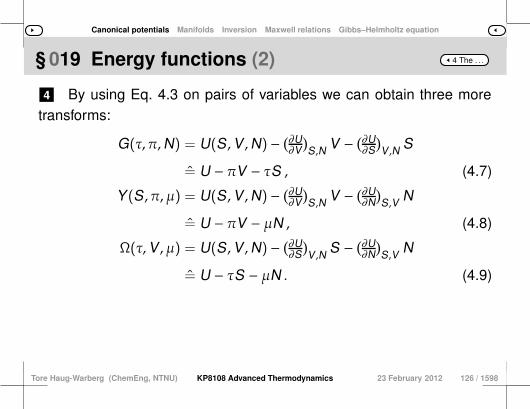
4 By using Eq. 4.3 on pairs of variables we can obtain three moretransforms:
G(τ, π,N) = U(S ,V ,N) − (∂U∂V
)S,N V − (∂U
∂S)V ,N S
= U − πV − τS , (4.7)
Y(S , π, µ) = U(S ,V ,N) − (∂U∂V
)S,N V − (∂U
∂N)S,V N
= U − πV − µN , (4.8)
Ω(τ,V , µ) = U(S ,V ,N) − (∂U∂S
)V ,N S − (∂U
∂N
)S,V N
= U − τS − µN . (4.9)
Tore Haug-Warberg (ChemEng, NTNU) KP8108 Advanced Thermodynamics 23 February 2012 126 / 1598

Canonical potentials Manifolds Inversion Maxwell relations Gibbs–Helmholtz equation
4 The . . .§ 019 Energy functions (3)
5 Finally, by using Eq. 4.2 on all three variables successivly we canobtain the null potential, which is also discussed on page 199 in Chap-ter 5:
O(τ, π, µ) = U(S ,V ,N) − (∂U∂V
)S,N V − (∂U
∂S
)V ,N S − (∂U
∂N
)S,V N
= U − πV − τS − µN
≡ 0 (4.10)
Tore Haug-Warberg (ChemEng, NTNU) KP8108 Advanced Thermodynamics 23 February 2012 127 / 1598
Canonical potentials Manifolds Inversion Maxwell relations Gibbs–Helmholtz equation
4 The . . .H A U G
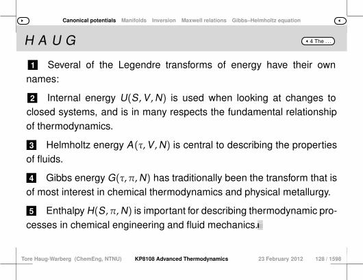
1 Several of the Legendre transforms of energy have their ownnames:
2 Internal energy U(S ,V ,N) is used when looking at changes toclosed systems, and is in many respects the fundamental relationshipof thermodynamics.
3 Helmholtz energy A(τ,V ,N) is central to describing the propertiesof fluids.
4 Gibbs energy G(τ, π,N) has traditionally been the transform that isof most interest in chemical thermodynamics and physical metallurgy.
5 Enthalpy H(S , π,N) is important for describing thermodynamic pro-cesses in chemical engineering and fluid mechanics.6 The grand canonical potential Ω(τ,V , µ) is used when describing
open systems in statistical mechanics.7 Meanwhile, the null potential O(τ, π, µ) has received less attention
than it deserves in the literature, and has no internationally acceptedname, even though the function has several interesting properties, aswe shall later see.8 This just leaves the two functions X(S , π, µ) and Y(S ,V , µ), which
are of no practical importance.9 However, it is worth mentioning that X is the only energy function
that has two, and always two, extensive variables no matter how manychemical components there are in the mixture.10 This function is therefore extremely well suited to doing stabilityanalyses of phase equilibria.11 In this case the basic geometry is simple, because the analysis isdone along a 2-dimensional manifold (a folded x, y plane) where thechemical potentials are kept constant.12 This topic is discussed further in a separate chapter on phase sta-bility.
Tore Haug-Warberg (ChemEng, NTNU) KP8108 Advanced Thermodynamics 23 February 2012 128 / 1598
Canonical potentials Manifolds Inversion Maxwell relations Gibbs–Helmholtz equation
4 The . . .§ 020 § 19 § 21
The variable ξj in Eq. 4.2 can be defined as either(∂φi/∂xj)ξi ,xk ,...,xn
or (∂f/∂xj)xi ,xk ,...,xn. Use implicit differentiation
to prove that the two definitions are equivalent.
Tore Haug-Warberg (ChemEng, NTNU) KP8108 Advanced Thermodynamics 23 February 2012 129 / 1598

Canonical potentials Manifolds Inversion Maxwell relations Gibbs–Helmholtz equation
4 The . . .§ 020 Differentiation I
1 2 Note that the variables xk , . . . , xn are common to both φi and f andmay hence be omitted for the sake of clarity.3 We will therefore limit our current analysis to the functions f(xi , xj)
and φi(ξi , xj). It is natural to start with Eq. 4.1, which we differentiate with respectto xj :
(∂φi∂xj
)ξi=
(∂(f−ξixi)∂xj
)ξi, (4.11)
where (∂ξi/∂xj)ξiis by definition zero.
4 Hence, at constant ξi:
d(f − ξixi)ξi=
( ∂f∂xi
)xj
dxi +( ∂f∂xj
)xi
dxj − ξi dxi
= ξi dxi +( ∂f∂xj
)xi
dxj − ξi dxi
=( ∂f∂xj
)xi
dxj
Tore Haug-Warberg (ChemEng, NTNU) KP8108 Advanced Thermodynamics 23 February 2012 130 / 1598

Canonical potentials Manifolds Inversion Maxwell relations Gibbs–Helmholtz equation
4 The . . .§ 020 Differentiation I (2)
6 5 or, alternatively:(d(f−ξi xi)
dxj
)ξi=
( ∂f∂xj
)xi. (4.12) The full derivative takes the same value as the corresponding par-
tial derivative (only one degree of freedom). Substitution into Eq. 4.11yields
(∂φi
∂xj
)ξi=
( ∂f∂xj
)xi= ξj (4.13)
leading to the conclusion that differentiation of φi with respect to theuntransformed variable xj gives the same derivative as for the originalfunction f .
Tore Haug-Warberg (ChemEng, NTNU) KP8108 Advanced Thermodynamics 23 February 2012 131 / 1598
Canonical potentials Manifolds Inversion Maxwell relations Gibbs–Helmholtz equation
4 The . . .§ 021 § 20 § 22 Before or after?1 It is a matter of personal preference, therefore, whether we want tocalculate ξj as (∂f/∂xj)xi
before the transformation is performed, or tocalculate (∂φi/∂xj)ξi
after the transformation has been defined.
2 Normally it is easiest to obtain all of the derivatives of the originalfunction first — especially when dealing with an explicitly defined ana-lytic function — but in thermodynamic analyses it is nevertheless usefulto bear both approaches in mind.
3 The next paragraph shows the alternative definitions we have fortemperature, pressure and chemical potential.
132 / 1598
Use the result from Paragraph 20 on page 122 toshow that the chemical potential has four equivalent
definitions: µ = (∂U/∂N)S,V = (∂H/∂N)S,π = (∂A/∂N)τ,V =
(∂G/∂N)τ,π. Specify the equivalent alternative definitionsfor temperature τ and negative pressure π.
Tore Haug-Warberg (ChemEng, NTNU) KP8108 Advanced Thermodynamics 23 February 2012 133 / 1598

Canonical potentials Manifolds Inversion Maxwell relations Gibbs–Helmholtz equation
4 The . . .§ 021 Identities I
1 Let f = U(S ,V ,N) be the function to be transformed. The questionasks for the derivatives with respect to the mole number N and it istacitly implied that only S and V are to be transformed.
2 From the Eqs. 4.4 and 4.5 we have φ1 = A(τ,V ,N) and φ2 = H(S ,π,N), which on substitution into Eq. 4.13 give:
(∂A∂N
)τ,V =
(∂U∂N
)S,V , (4.14)
(∂H∂N
)S,π =
(∂U∂N
)S,V . (4.15)
3 The transform φ12 = φ21 = G(τ, π,N) in Eq. 4.7 can be reachedeither via A or H.
Tore Haug-Warberg (ChemEng, NTNU) KP8108 Advanced Thermodynamics 23 February 2012 134 / 1598
Canonical potentials Manifolds Inversion Maxwell relations Gibbs–Helmholtz equation
4 The . . .§ 021 Identities I (2)
4 Inserted into Eq. 4.13 the two alternatives become:(∂G∂N
)τ,π
=(∂A∂N
)τ,V , (4.16)
(∂G∂N
)τ,π
=(∂H∂N
)S,π . (4.17)
7 5 Note that all the Eqs. 4.14–4.17 have one variable in common onthe left and right hand sides (V , S, τ and π respectively).6 For multicomponent systems this variable will be a vector; cf. xk ,
. . . , xn in Paragraph 20. So, in conclusion, the following is true for any single-componentsystem:
µ =(∂A∂N
)τ,V =
(∂H∂N
)S,π =
(∂G∂N
)τ,π
=(∂U∂N
)S,V . (4.18)
8 By performing the same operations on temperature and negativepressure we obtain:
τ =(∂H∂S
)π,N =
(∂X∂S
)V ,µ =
(∂Y∂S
)π,µ
=(∂U∂S
)V ,N , (4.19)
π =(∂A∂V
)τ,N =
(∂X∂V
)S,µ =
(∂Ω∂V
)τ,µ
=(∂U∂V
)S,N (4.20)
Tore Haug-Warberg (ChemEng, NTNU) KP8108 Advanced Thermodynamics 23 February 2012 135 / 1598

Canonical potentials Manifolds Inversion Maxwell relations Gibbs–Helmholtz equation
4 The . . .§ 021 Identities I (3)
Tore Haug-Warberg (ChemEng, NTNU) KP8108 Advanced Thermodynamics 23 February 2012 136 / 1598

Canonical potentials Manifolds Inversion Maxwell relations Gibbs–Helmholtz equation
4 The . . .§ 022 § 21 § 23 Freedom to choose1 This shows very clearly that we are free to choose whatever co-ordinates we find most convenient for the description of the physicalproblem we want to solve.
2 For example, in chemical equilibrium theory it is important to knowthe chemical potentials of each component in the mixture.
3 If the external conditions are such that temperature and pressureare fixed, it is natural to use µi = (∂G/∂Ni)T ,p,Nj,i , but if the entropyand pressure are fixed, as is the case for reversible and adiabatic statechanges, then µi = (∂H/∂Ni)S,p,Nj,i is a more appropriate choice.
137 / 1598
The Legendre transform was differentiated with respectto the orginal variable xj in Paragraph 20. However, the
derivative with respect to the transformed variable ξi
remains to be determined. Show that (∂φi/∂ξi)xj ,xk ,...,xn
= −xi.
Tore Haug-Warberg (ChemEng, NTNU) KP8108 Advanced Thermodynamics 23 February 2012 138 / 1598
Canonical potentials Manifolds Inversion Maxwell relations Gibbs–Helmholtz equation
4 The . . .§ 022 Differentiation II
1 2 As in Paragraph 20, the variables xk , . . . , xn are common to both fand φi, and have therefore been omitted for the sake of clarity. Let us start with φi(ξi , xj) = f(xi , xj)−ξixi from Eq. 4.1 and differen-
tiate it with respect to ξi. Note that the chain rule of differentiation( ∂f∂ξi
)xj=
( ∂f∂xi
)xj
(∂xi∂ξi
)xj
has been used to obtain the last line below:(∂φi∂ξi
)xj=
( ∂f∂ξi
)xj− (∂(ξixi)
∂ξi
)xj
=( ∂f∂ξi
)xj− xi − ξi
(∂xi∂ξi
)xj
=( ∂f∂xi
)xj
(∂xi∂ξi
)xj− xi − ξi
(∂xi∂ξi
)xj. (4.21)
Tore Haug-Warberg (ChemEng, NTNU) KP8108 Advanced Thermodynamics 23 February 2012 139 / 1598
Canonical potentials Manifolds Inversion Maxwell relations Gibbs–Helmholtz equation
4 The . . .§ 022 Differentiation II (2)
3 From Eq. 4.3 we know that (∂f/∂xi)xj= ξi, which can easily be
substituted into Eq. 4.21 to produce(∂φi∂ξi
)xj= −xi , (4.22)
which leads to the following conclusion: The derivative of φi with respectto a transformed variable ξi is the original variable xi, but with the signreversed.4 In other words, there is a special relationship between the variables
xi in f(xi , xj) and ξi in φi(ξi , xj)a.5 Due to the simple relationship set out in Eq. 4.22, the variables (ξi ,
xj) are said to be the canonical variables of φi(ξi , xj).
a The variables x and ξ are said to be conjugate variables.
Tore Haug-Warberg (ChemEng, NTNU) KP8108 Advanced Thermodynamics 23 February 2012 140 / 1598

Canonical potentials Manifolds Inversion Maxwell relations Gibbs–Helmholtz equation
4 The . . .Non-canonical differentiation
1 The Eq. 4.22 is strikingly simple, and leads to a number of simplifi-cations in thermodynamics.
2 The properties explained in the previous paragraph are of primeimportance. Before we move on, however, we should investigate whathappens if we do not describe the Legendre transform in terms ofcanonical variables.
3 Differentiating φi = f − ξixi with respect to the original varibale xi
gives:(∂φi∂xi
)xj,i
=( ∂f∂xi
)xj,i− (∂ξi
∂xi
)xj,i
xi − ξi = −( ∂2f∂xi∂xi
)xj,i
xi ,
Tore Haug-Warberg (ChemEng, NTNU) KP8108 Advanced Thermodynamics 23 February 2012 141 / 1598

Canonical potentials Manifolds Inversion Maxwell relations Gibbs–Helmholtz equation
4 The . . .§ 023 § 22 § 24Non-canonical differentiation1 The expression on the right-hand side is not particularly complex,
but unfortunately it is not canonically related to f . It is nevertheless animportant result, because φi must by definition be a function with thesame variables as f itself.
2 The change in variable from xi to ξi is an abstract concept that willonly rarely produce an explicit expression stated in terms of ξi .
3 Hence, if we want to calculate the derivative of φi by means ofan explicit function, we have to go via f and its derivatives — there issimply no way around it. A simple example shows how and why this isthe case:
(∂U∂T
)V ,N = − ( ∂2A
∂T∂T)V ,N T =
(∂S∂T
)V ,N T =
CV
T T = CV(T ,V ,N) .
4 Here the internal energy is, at least formally speaking, a function ofthe canonical variables S, V and N, but there are virtually no equationsof state that are based on these variables.
5 T , V and N are much more common in that context, so to lure Uinto revealing its secrets we must use T rather S.
6 Note, however, that in this case S = − (∂A/∂T)V ,N is a function tobe differentiated and not a free variable.
7 This illustrates in a nutshell the challenges we face in thermody-namics: Variables and functions are fragile entities with changing in-terpretations depending on whether we want to perform mathematicalanalyses or numerical calculations.
142 / 1598
Use the results obtained in Paragraph 22 to prove thatthe derivatives (∂H/∂π)S,N, (∂G/∂π)τ,N and (∂Y/∂π)S,µ
are three equivalent ways of expressing the volume Vof the system. Specify the corresponding expressions
for the entropy S and the mole number N.
Tore Haug-Warberg (ChemEng, NTNU) KP8108 Advanced Thermodynamics 23 February 2012 143 / 1598

Canonical potentials Manifolds Inversion Maxwell relations Gibbs–Helmholtz equation
4 The . . .§ 023 Identities II
1 Let us start out once more from f = U(S ,V ,N) and define4 thetransform φ2 = H(S , π,N) = U − πV . Inserted into Eq. 4.22, this givesus (∂H/∂π)S,N = −V .
2 Systematically applying Eq. 4.22 to all of the energy functions inParagraph 19 on page 117 yields5:
−V =(∂H∂π
)S,N =
(∂G∂π
)τ,N =
(∂Y∂π
)S,µ , (4.23)
−S =(∂A∂τ
)V ,N =
(∂G∂τ
)π,N =
(∂Ω∂τ
)V ,µ , (4.24)
−N =(∂X∂µ
)S,V
=(∂Y∂µ
)S,π
=(∂Ω∂µ
)τ,V
. (4.25)
Tore Haug-Warberg (ChemEng, NTNU) KP8108 Advanced Thermodynamics 23 February 2012 144 / 1598
Canonical potentials Manifolds Inversion Maxwell relations Gibbs–Helmholtz equation
4 The . . .§ 023 Identities II (2)
4 The symbol π = −p is used here as the pressure variable. This is quite deliberate,in order to avoid the eternal debate about the sign convention for p. As used here,τ, π and µ are subject to the same transformation rules. This means that the samerules apply to e.g. (∂H/∂π)S ,N = −V and (∂A/∂τ)V ,N = −S, whereas the traditionalapproach using (∂H/∂p)S ,N = V and (∂A/∂T)V ,N = −S involves different rules for pand T derivatives. Note, however, that it makes no difference whether −p or p is keptconstant during the differentiation.5 Sharp students will note the absence of −S = (∂O/∂τ)π,µ, V = (∂O/∂π)τ,µ and −N =
(∂O/∂µ)τ,p . These relations have no clear thermodynamic interpretation, however,because experimentally τ, π, µ are dependent variables, see also Paragraph 26 onpage 157.
Tore Haug-Warberg (ChemEng, NTNU) KP8108 Advanced Thermodynamics 23 February 2012 145 / 1598
Canonical potentials Manifolds Inversion Maxwell relations Gibbs–Helmholtz equation
4 The . . .§ 024 § 23 § 25 Systematics1 Knowing the properties of the Legendre transform, as expressed
by Eqs. 4.13 and 4.22, allows us to express all of the (energy) functionsU, H, A , . . . O that we have considered so far in terms of their canonicalvariables.
2 The pattern that lies hidden in these equations can easily be con-densed into a table of total differentials for each of the functions (seebelow).
146 / 1598
Use the results from Paragraphs 21 and 23 on pages125 and 133 to find the total differentials of all the
energy functions mentioned in Paragraph 19.
Tore Haug-Warberg (ChemEng, NTNU) KP8108 Advanced Thermodynamics 23 February 2012 147 / 1598

Canonical potentials Manifolds Inversion Maxwell relations Gibbs–Helmholtz equation
4 The . . .§ 024 Differentials I
1 The total differentials of the energy functions can be stated by tak-ing the results from Eqs. 4.18–4.20 and 4.23–4.25 as a starting point:
dU (S ,V ,N) = τ dS + π dV + µ dN , (4.26)
dA (τ ,V ,N) = −S dτ + π dV + µ dN , (4.27)
dH (S , π,N) = τ dS − V dπ + µ dN , (4.28)
dX (S ,V , µ) = τ dS + π dV −N dµ , (4.29)
dG (τ , π,N) = −S dτ − V dπ + µ dN , (4.30)
dY (S , π, µ) = τ dS − V dπ −N dµ , (4.31)
dΩ (τ ,V , µ) = −S dτ + π dV −N dµ , (4.32)
dO (τ , π, µ) = −S dτ − V dπ −N dµ . (4.33)
Tore Haug-Warberg (ChemEng, NTNU) KP8108 Advanced Thermodynamics 23 February 2012 148 / 1598
Canonical potentials Manifolds Inversion Maxwell relations Gibbs–Helmholtz equation
4 The . . .Manifolds
1 In what has been written so far we note that all of the state variablesτ, S, π, V , µ and N appear in conjugate pairs such as τdS, −S dτ,πdV , −V dπ, µ dN or −N dµ.
3 2 This is an important property of the energy functions. The obvious symmetry reflects Eq. 4.22, which also implies thatthe Legendre transform is “its own inverse”.
4 However, this is only true if the function is either strictly convexor strictly concave, as the relationship breaks down when the secondderivative f(xi , xj , xk , . . . , xn) is zero somewhere within the domain ofdefinition of the free variables (see also Section 4.3).
Tore Haug-Warberg (ChemEng, NTNU) KP8108 Advanced Thermodynamics 23 February 2012 149 / 1598
Canonical potentials Manifolds Inversion Maxwell relations Gibbs–Helmholtz equation
4 The . . .Manifolds (2)
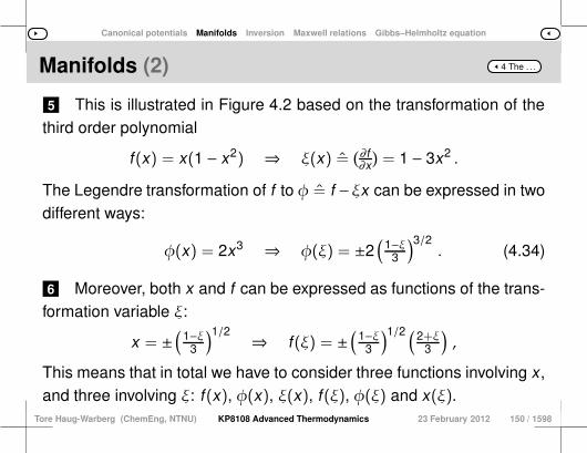
5 This is illustrated in Figure 4.2 based on the transformation of thethird order polynomial
f(x) = x(1 − x2) ⇒ ξ(x) =(∂f∂x)= 1 − 3x2 .
The Legendre transformation of f to φ = f −ξx can be expressed in twodifferent ways:
φ(x) = 2x3 ⇒ φ(ξ) = ±2(
1−ξ3
)3/2. (4.34)
6 Moreover, both x and f can be expressed as functions of the trans-formation variable ξ:
x = ±(
1−ξ3
)1/2⇒ f(ξ) = ±
(1−ξ
3
)1/2 (2+ξ
3
),
This means that in total we have to consider three functions involving x,and three involving ξ: f(x), φ(x), ξ(x), f(ξ), φ(ξ) and x(ξ).
Tore Haug-Warberg (ChemEng, NTNU) KP8108 Advanced Thermodynamics 23 February 2012 150 / 1598
Canonical potentials Manifolds Inversion Maxwell relations Gibbs–Helmholtz equation
4 The . . .Manifolds (3)
7 In order to retain the information contained in f(x), we need to knoweither φ(x) and ξ(x), or f(ξ) and x(ξ), or simply φ(ξ). In principle, thelatter is undoubtedly the best option, and this is the immediate reasonwhy φ(ξ) is said to be in canonical form.
8 Nevertheless, there is an inversion problem when φ is interpretedas a function of ξ rather than x.
10 9 This is clearly demonstrated by the above example, where x is anambiguous function of ξ, which means that φ(ξ), and similarly f(ξ), arenot functions in the normal sense. Instead, they are examples of what we call manifolds (loosely
speaking folded surfaces defined by a function) as illustrated in Fig-ures 4.2c–4.2d6.
6 A function is a point-to-point rule that connects a point in the domain of definition witha corresponding point in the function range.
Tore Haug-Warberg (ChemEng, NTNU) KP8108 Advanced Thermodynamics 23 February 2012 151 / 1598

Canonical potentials Manifolds Inversion Maxwell relations Gibbs–Helmholtz equation
4 The . . .Consistency requirements
1 Finally, let us look at what differentiating φ with respect to ξ implies.From Section 22, we know that the answer is −x, but
(∂φ
∂ξ
)= ∓
(1−ξ
3
)1/2
initially gives us a manifold in ξ with two solutions, as shown in Fig-ure 4.2.
2 It is only when we introduce x(ξ) from Eq. 4.34 that the full pictureemerges: (∂φ/∂ξ) = −x.
5 3 This does not mean that we need x(ξ) to calculate the values of(∂φ/∂ξ).4 However, the relationship between x, ξ and (∂φ/∂ξ) is needed for
system identification. If the three values have been independently measured, then therelation (∂φ/∂ξ) = −x can be used to test the experimental values forconsistency.
Tore Haug-Warberg (ChemEng, NTNU) KP8108 Advanced Thermodynamics 23 February 2012 152 / 1598

Canonical potentials Manifolds Inversion Maxwell relations Gibbs–Helmholtz equation
4 The . . .Consistency requirements (2)
6 The existence of these kinds of tests, which can involve a variety ofphysical measurements, is one of the great strengths of thermodynam-ics.
Tore Haug-Warberg (ChemEng, NTNU) KP8108 Advanced Thermodynamics 23 February 2012 153 / 1598

Canonical potentials Manifolds Inversion Maxwell relations Gibbs–Helmholtz equation
Figure a–b). The function f = x(1 −x2) and its Legendre transform φ =
2x3 defined as the intersection of thetangent bundle of f and the ordinateaxis. Note that f shows a maximumand a minimum while φ has no ex-trema.
x
f(x)
a)
x
φ(x)
b)
ξ
f(ξ)
c)
ξ
φ(ξ)
d)
Figure c–d). The same two functionsshown as parametric curves with ξ =
(∂f/∂x) = 1−3x2 along the abscissa.The fold in the plane(s) is located atthe inflection point (∂2f/∂x∂x) = 0.
Figure 4.2: The Legendre transformation of f = x(1− x2) to φ = f − ξx whereξ = (∂f/∂x) = 1 − 3x2. The two domains of definition are x ∈ [−
√2/3,
√2/3]
and ξ ∈ [−1, 1]. Together, the four graphs demonstrate how an explicit functionof x, i.e. f(x) or φ(x), is turned into an implicit manifold when expressed interms of ξ, i.e. f(ξ) or φ(ξ).
Tore Haug-Warberg (ChemEng, NTNU) KP8108 Advanced Thermodynamics 23 February 2012 154 / 1598
Canonical potentials Manifolds Inversion Maxwell relations Gibbs–Helmholtz equation
4 The . . .Vapour–liquid
1 2 The above example also has practical relevance.3 Many equations of state, and particularly those for the fluid state,
are explicit equations of the form p = p(T ,V ,N).4 These equations of state can be used to calculate the Helmholtz
energy of the fluid.5 The problem in relation to manifolds becomes clear when this en-
ergy is transformed into Gibbs energy, which requires us to know theterm V = V(p) in the definition G(p) = A(V(p)) + pV(p).6 Along the sub-critical isotherms the relation V = V(p) is equivalent
to a manifold with 3 roots as illustrated in Figure 14.6 on page 736.7 This results in a characteristic folding of the energy surface as ex-
amplified by the p, µ diagram in Figure 14.2 on page 708; where themolar volume v is used as a parameter for p(v) along the abscissa andfor µ(v) along the ordinate axis. In view of these practical considerations, we cannot claim that Leg-
endre transforms are globally invertible, but it is true to say that theyare locally invertible on curve segments where the sign of (∂2f/∂x∂x)remains unchanged. We shall therefore take the precaution of treatingeach curve segment as a separate function.
8 For instance, in vapor–liquid equilibrium calculations we shall des-ignate one of the curve segments as being vapour and the other as be-ing liquid, although there is no thermodynamic justification for this dis-tinction, other than the fact that (∂2A/∂V∂V)T ,N = 0 somewhere alongthe isotherm.
Tore Haug-Warberg (ChemEng, NTNU) KP8108 Advanced Thermodynamics 23 February 2012 155 / 1598

Canonical potentials Manifolds Inversion Maxwell relations Gibbs–Helmholtz equation
4 The . . .From φ to f ?
1 In this section we will explain how, and under what conditions, itis possible to convert the Legendre transform φ back to the originalfunction f .
2 This operation will be based on the transformation rule set out inEq. 4.1
φ(y) = f − (∂f∂x
)x , (4.35)
where the properties of the variable y are, as yet, unknown.
Tore Haug-Warberg (ChemEng, NTNU) KP8108 Advanced Thermodynamics 23 February 2012 156 / 1598
Canonical potentials Manifolds Inversion Maxwell relations Gibbs–Helmholtz equation
4 The . . .From φ to f ? (2)
3 What we need to know is whether the same transformation ruleapplies to the inverse transform of φ(y), such that
f ?= φ − (∂φ
∂y
)y , (4.36)
and, if so, what y is (we have an inkling that y = (∂f/∂x), but we needto prove it).
4 Substituting Eq. 4.36 into Eq. 4.35, rearranging the expressionslightly, and applying the chain rule, gives us:
− (∂φ∂y
)y = − (∂φ
∂x) (∂x∂y
)y ?=
(∂f∂x
)x . (4.37)
Tore Haug-Warberg (ChemEng, NTNU) KP8108 Advanced Thermodynamics 23 February 2012 157 / 1598

Canonical potentials Manifolds Inversion Maxwell relations Gibbs–Helmholtz equation
4 The . . .From φ to f ? (3)
5 Next we substitute Eq. 4.35 into Eq. 4.37:
−((∂f∂x) − ( ∂2f
∂x∂x)x − (∂f
∂x)) (∂x
∂y)y ?=
(∂f∂x
)x
( ∂2f∂x∂x
)x(∂x∂y)y ?=
(∂f∂x
)x
(∂x∂y)y ?=
(∂f∂x
) ( ∂2f∂x∂x
)-1. (4.38)
Tore Haug-Warberg (ChemEng, NTNU) KP8108 Advanced Thermodynamics 23 February 2012 158 / 1598
Canonical potentials Manifolds Inversion Maxwell relations Gibbs–Helmholtz equation
4 The . . .Integration
1 For the inverse transform to exist, it must be true that (∂2f/∂x∂x) ,0. This is a necessary condition.
2 It is also worth adding that in general, partial differential equationsdo not have an analytical solution. However, thermodynamic problemsare often unusually simple, and that is also the case here.
3 Let us define ξ = (∂f/∂x), which gives us(∂x∂y
)y ?= ξ
(∂ξ∂x
)-1.
Tore Haug-Warberg (ChemEng, NTNU) KP8108 Advanced Thermodynamics 23 February 2012 159 / 1598

Canonical potentials Manifolds Inversion Maxwell relations Gibbs–Helmholtz equation
4 The . . .Integration (2)
4 Introducing the logarithmic variables dln y = dy /y and dln ξ =
dξ /ξ produces an elegant solution to the problem (note how the chainrule is used in reverse in the second-last line):
( ∂x∂ ln y
)=
(∂ ln ξ∂x
)-1(∂ lnξ∂x
) ( ∂x∂ ln y
)= 1
(∂ ln ξ∂ ln y
)= 1 (4.39)
Tore Haug-Warberg (ChemEng, NTNU) KP8108 Advanced Thermodynamics 23 February 2012 160 / 1598
Canonical potentials Manifolds Inversion Maxwell relations Gibbs–Helmholtz equation
4 The . . .Solution criteria
1 The most general solution can be expressed as y = cξ =
c (∂f/∂x), where c is an arbitrary factor. It is natural to choose c = 1,which means that y ≡ ξ, as we know from our earlier discussion of theLegendre transform, but any value of c ∈ R+ will give the same result,as the inverse transformin Eq. 4.36 is insensitive to scaling.
2 We say that x and ξ are the natural (or canonical) variables of thefunctions f(x) and φ(ξ), as they allow transformation in both directionswithout the loss of any information.
4 3 As an aside, it should be mentioned that the function φ(x) does nothave this property, because y = x is not a solution to Eq. 4.36. In the context of thermodynamics, this means that e.g.
A(T ,V ,n) can be inverse transformed to U(S ,V ,n), provided that(∂2U/∂S∂S)V ,n , 0.
Tore Haug-Warberg (ChemEng, NTNU) KP8108 Advanced Thermodynamics 23 February 2012 161 / 1598

Canonical potentials Manifolds Inversion Maxwell relations Gibbs–Helmholtz equation
4 The . . .Solution criteria (2)
5 However, the transformation rule is symmetrical, and the same re-quirement must also apply in the other direction: U(S ,V ,n) can only betransformed into A(T ,V ,n) if (∂2A/∂T∂T)V ,n , 0.
6 The two requirements may appear contradictory, but in actual factthey are overlapping, because:
( ∂2U∂S∂S
)V ,n =
(∂T∂S
)V ,n =
(∂S∂T
)-1V ,n = − ( ∂2A
∂T∂T
)-1V ,n
7 In states in which one of the derivatives tends to zero, and the otherone tends to infinity, the system is on the verge of being unstable.
8 Depending on the variables involved, this relates to either thermal(T , S), mechanical (p, V ) or chemical (µi, Ni) stability.9 These kinds of states are always buried inside a region with two or
more phases, being found in what is referred to as the spinodal regionof the system (from the gr. spinode, meaning “cusp”).
Tore Haug-Warberg (ChemEng, NTNU) KP8108 Advanced Thermodynamics 23 February 2012 162 / 1598

Canonical potentials Manifolds Inversion Maxwell relations Gibbs–Helmholtz equation
4 The . . .§ 025 § 24 § 26
Use the result from Paragraph 22 on page 129 toshow that performing two Legendre transformationson f , first with respect to xi and then with respect to
ξi, returns the original function.
Tore Haug-Warberg (ChemEng, NTNU) KP8108 Advanced Thermodynamics 23 February 2012 163 / 1598
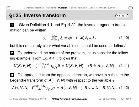
Canonical potentials Manifolds Inversion Maxwell relations Gibbs–Helmholtz equation
4 The . . .§ 025 Inverse transform
1 Given Definition 4.1 and Eq. 4.22, the inverse Legendre transfor-mation can be written
φi −(∂φi∂ξi
)xjξi = φi − (−xi)ξi ≡ f , (4.40)
but it is not entirely clear what variable set should be used to define f .
2 To understand the nature of the problem, let us consider the follow-ing example. From Eq. 4.4 it follows that:
U(S ,V ,N) − (∂U(S,V ,N)∂S
)V ,N S = U(S ,V ,N) − τS = A(τ,V ,N) . (4.41)
3 To approach it from the opposite direction, we have to calculate theLegendre transform of A(τ,V ,N) with respect to the variable τ:
A(τ,V ,N)−(∂A(τ,V ,N)∂τ
)V ,N τ = A(τ,V ,N)−(−S)τ ≡ U(−S ,V ,N) . (4.42)
Tore Haug-Warberg (ChemEng, NTNU) KP8108 Advanced Thermodynamics 23 February 2012 164 / 1598
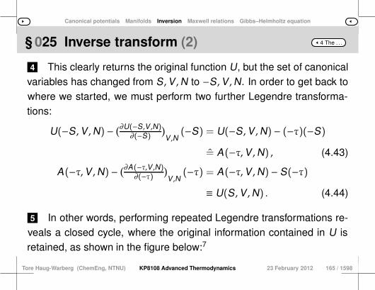
Canonical potentials Manifolds Inversion Maxwell relations Gibbs–Helmholtz equation
4 The . . .§ 025 Inverse transform (2)
4 This clearly returns the original function U, but the set of canonicalvariables has changed from S ,V ,N to −S ,V ,N. In order to get back towhere we started, we must perform two further Legendre transforma-tions:
U(−S ,V ,N) − (∂U(−S,V ,N)∂(−S)
)V ,N
(−S) = U(−S ,V ,N) − (−τ)(−S)
= A(−τ,V ,N) , (4.43)
A(−τ,V ,N) − (∂A(−τ,V ,N)∂(−τ)
)V ,N
(−τ) = A(−τ,V ,N) − S(−τ)
≡ U(S ,V ,N) . (4.44)
5 In other words, performing repeated Legendre transformations re-veals a closed cycle, where the original information contained in U isretained, as shown in the figure below:7
Tore Haug-Warberg (ChemEng, NTNU) KP8108 Advanced Thermodynamics 23 February 2012 165 / 1598
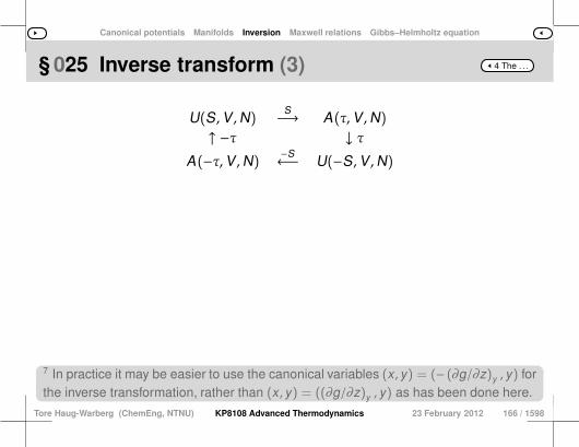
Canonical potentials Manifolds Inversion Maxwell relations Gibbs–Helmholtz equation
4 The . . .§ 025 Inverse transform (3)
U(S,V ,N)S−→ A(τ,V ,N)
↑ −τ ↓ τA(−τ,V ,N)
−S←− U(−S,V ,N)
7 In practice it may be easier to use the canonical variables (x , y) = (− (∂g/∂z)y , y) forthe inverse transformation, rather than (x , y) = ((∂g/∂z)y , y) as has been done here.
Tore Haug-Warberg (ChemEng, NTNU) KP8108 Advanced Thermodynamics 23 February 2012 166 / 1598

Canonical potentials Manifolds Inversion Maxwell relations Gibbs–Helmholtz equation
4 The . . .Invertibility
1 This example shows that the Legendre transform is (locally) invert-ible, which means that we can choose whatever energy function is mostsuitable for our purposes.
2 Moreover, Eq. 4.10 tells us that the Legendre transform of U withrespect to all of the state variables S, V and N is a function with veryspecial properties. The function, which is known as the null potential, isidentical to zero over the entire definition domain, and as such it has noinverse.3 Our line of reasoning breaks down for this function, and we must
expect O(T , p, µ) to have properties that differ from those of U and theother energy functions.4 Note that this is not a general mathematical property of the Leg-
endre transform; rather it follows inevitably from the fact that U and allof the other extensive properties are described by first-order homoge-neous functions to which Euler’s theorem can be applied.5 These functions display a kind of linearity that results in their total
Legendre transforms being identical to zero.6 Hence, the differentials are also zero over the entire definition do-
main.7 In thermodynamics, this is called the Gibbs–Duhem equation.
Tore Haug-Warberg (ChemEng, NTNU) KP8108 Advanced Thermodynamics 23 February 2012 167 / 1598

Canonical potentials Manifolds Inversion Maxwell relations Gibbs–Helmholtz equation
4 The . . .§ 026 § 25 § 27
Show that performing a Legendre transformation ofinternal energy U(S ,V ,N) with respect to all the canonical
variables S ,V ,N gives the null potential O(τ, π, µ) =
0. Next, show that the differential of O is identical tothe Gibbs–Duhem equation; see also Paragraph 34
in Chapter 5.
Tore Haug-Warberg (ChemEng, NTNU) KP8108 Advanced Thermodynamics 23 February 2012 168 / 1598
Canonical potentials Manifolds Inversion Maxwell relations Gibbs–Helmholtz equation
4 The . . .§ 026 Null potential
1 2 The differential of the null potential in Eq. 4.10 is of course 0. However, since this result is valid for the entire domain of definitionit must have a bearing on the degrees of freedom of the system.
3 Mathematically, the O-function forms a hyperplane in dim(n) + 2dimensions.4 This becomes clear if we differentiate O(τ, π, µ) in Eq. 4.10: dU −
τdS − S dτ − V dπ − πdV − µ dN − N dµ = 0.5 If we spot that τdS +πdV +µ dN is the total differential of internalenergy, we can simplify the expression to:
S dτ+ V dπ+ N dµ = 0 . (4.45)
6 This result is identical to the Gibbs–Duhem Eq. 5.23, which playsan important role in checking the thermodynamic consistency of exper-imental data.7 This is because Eq. 4.45 tells us about the relationship between τ,π, µ.8 If a series of measurements is taken in order to obtain experimentalvalues for all of the variables τ, π, µ, then the Gibbs–Duhem equationallows us to check the quality of the measurements, given that Eq. 4.45,or Eq. 4.10 for that matter, must be fulfilled.9 In practice, this is possible because the chemical potentiala,
10 can be expressed as a function of temperature and negative pres-sure, or alternatively as f(τ, π, µ) = 0.
a For single component or multicomponent systems at fixed concentration.
Tore Haug-Warberg (ChemEng, NTNU) KP8108 Advanced Thermodynamics 23 February 2012 169 / 1598
Canonical potentials Manifolds Inversion Maxwell relations Gibbs–Helmholtz equation
4 The . . .Seven samurai
1 We have in this chapter introduced seven energy functions: U, H,A , G, X , Y and O , and six state variables: S, V , N, t , p and µ.
2 On reflection it is clear that only four of these variables are inde-pendent, because the discussion has relied entirely on the fact that in-ternal energy U is a function of S, V and N.
3 All of the other varaibles have been defined at a later stage eitheras partial derivatives or as transformed functions of U.4 There is therefore a substantial degree of redundancy in the vari-
ables that we are dealing with.5 This redundancy becomes even clearer when the energy functions
are differentiated twice with respect to their canonical variables.
Tore Haug-Warberg (ChemEng, NTNU) KP8108 Advanced Thermodynamics 23 February 2012 170 / 1598

Canonical potentials Manifolds Inversion Maxwell relations Gibbs–Helmholtz equation
4 The . . .§ 027 § 26 § 28
Set out all of the Maxwell relations that can be derivedby applying the Leibniz8 rule ∂2f/∂xi∂xj = ∂2f/∂xj∂xi
to the functions U,A ,H,Y ,G,Ω,X and O , restrictingyourself to single-component systems.
8 Gottfried Wilhelm von Leibniz, 1646–1716. German mathematician.
Tore Haug-Warberg (ChemEng, NTNU) KP8108 Advanced Thermodynamics 23 February 2012 171 / 1598

Canonical potentials Manifolds Inversion Maxwell relations Gibbs–Helmholtz equation
4 The . . .§ 027 Maxwell relations
1 Let us begin by illustrating what is meant by a Maxwell9 relationusing U(S ,V ,N) as our starting point. From the definitions of τ and π itfollows that:
( ∂2U∂S∂V
)N =
( ∂2U∂V∂S
)N ⇒
[∂∂S
(∂U∂V
)S,N
]V ,N
=[∂∂V
(∂U∂S
)V ,N
]S,N
⇒ (∂π∂S
)V ,N =
(∂τ∂V
)S,N .
2 Similarly, cyclic permutation of the variables S ,V and N yields:( ∂2U∂S∂N
)V =
( ∂2U∂N∂S
)V ⇒ (∂µ
∂S)V ,N =
(∂τ∂N
)S,V ,
( ∂2U∂V∂N
)S =
( ∂2U∂N∂V
)S ⇒ (∂µ
∂V
)S,N =
(∂π∂N
)S,V .
3 By systematically comparing the second derivatives of all of theLegendre transforms mentioned in Paragraph 19 on page 117, we getthe results shown below.
Tore Haug-Warberg (ChemEng, NTNU) KP8108 Advanced Thermodynamics 23 February 2012 172 / 1598

Canonical potentials Manifolds Inversion Maxwell relations Gibbs–Helmholtz equation
4 The . . .§ 027 Maxwell relations (2)
5 4 Also see Paragraph 24 on page 136 for a complementary table oftotal differentials and first derivatives. Note that the Maxwell relations which are derived from the null
potential O(τ, π, µ) have no physical interpretation, as experimentally τ,π, µ are dependent variables.6 This means that e.g. (∂τ/∂π)µ is unpredictable because Eq. 4.45
on integrated form is equivalent to a relation g such that g(τ, π, µ) = 0.7 These relations have therefore been omitted from the table.
(∂π∂S
)V ,N=
(∂τ∂V
)S,N
(∂µ∂S
)V ,N=
(∂τ∂N
)S,V
(∂µ∂V
)S,N=
(∂π∂N
)S,V
− (∂S∂V
)τ,N =
(∂π∂τ
)V ,N − (∂S
∂N)τ,V =
(∂µ∂τ
)V ,N
(∂π∂N
)τ,V =
(∂µ∂V
)τ,N
− (∂τ∂π
)S ,N=
(∂V∂S
)π,N
(∂τ∂N
)S ,π=
(∂µ∂S
)π,N − (∂V
∂N)S,π=
(∂µ∂π
)S,N(∂τ
∂V)S ,µ=
(∂π∂S
)V ,µ − (∂τ
∂µ
)S ,V
=(∂N∂S
)V ,µ − (∂π
∂µ
)S,V
=(∂N∂V
)S,µ
(∂S∂π
)τ,N =
(∂V∂τ
)π,N − (∂S
∂N)τ,π =
(∂µ∂τ
)π,N − (∂V
∂N)τ,π =
(∂µ∂π
)τ,N
− (∂τ∂π
)S ,µ =
(∂V∂S
)π,µ − (∂τ
∂µ
)S ,π
=(∂N∂S
)π,µ
(∂V∂µ
)S,π
=(∂N∂π
)S,µ
− (∂S∂V
)τ,µ =
(∂π∂τ
)V ,µ
(∂S∂µ
)τ,V
=(∂N∂τ
)V ,µ − (∂π
∂µ
)τ,V
=(∂N∂V
)τ,µ
9 James Clerk Maxwell, 1831–1879. Scottish physicist.
Tore Haug-Warberg (ChemEng, NTNU) KP8108 Advanced Thermodynamics 23 February 2012 173 / 1598

Canonical potentials Manifolds Inversion Maxwell relations Gibbs–Helmholtz equation
4 The . . .Alternative procedure
1 We are familiar with the key characteristics of Legendre trans-forms, having looked at topics like transformation geometry, differen-tiation rules, inverse transforms and Maxwell relations. We shall nowfocus on the simple rule used in Figure 4.1, which shows that the Leg-endre transform is equal to the intersection of the tangent bundle of theoriginal function and the ordinate axis.
2 The subject becomes even more interesting now, as we are goingto prove another rule, which is even simpler, although not so easy toderive. The key to this is a simple change in variables from y and x in(∂y/∂x) to y/x and 1/x in the expression (∂(y/x)/∂(1/x)).3 This relationship is generally known as the Gibbs–Helmholtz equa-
tion.
Tore Haug-Warberg (ChemEng, NTNU) KP8108 Advanced Thermodynamics 23 February 2012 174 / 1598
Canonical potentials Manifolds Inversion Maxwell relations Gibbs–Helmholtz equation
4 The . . .§ 028 § 27 § 29
Verify the Gibbs–Helmholtz equation (∂(G/τ)/∂(1/τ))π,N ≡ H.See if you can generalise this result.
Tore Haug-Warberg (ChemEng, NTNU) KP8108 Advanced Thermodynamics 23 February 2012 175 / 1598

Canonical potentials Manifolds Inversion Maxwell relations Gibbs–Helmholtz equation
4 The . . .§ 028 Gibbs–Helmholtz
1 2 By differentiating and then substituting (∂G/∂τ)π,N = −S and G +
TS = H, we can confirm that the equation is correct, but there is moreto it than that. From the mathematical identity
∂(y/x)∂(1/x) ≡ y + 1
x∂y
∂(1/x) ≡ y − x ∂y∂x
we can conclude that(∂(f/xi)∂(1/xi)
)xj ,xk ,...,xn
= f − ξixi = φi , (4.46)
cf. the Legendre transform in Eq. 4.1. The identity applies generally,including to φij and to any other derived transforms.
4 3 This means that Eq. 4.46 provides an alternative way of calculatingthe value of a Legendre transform, without this changing the originaldefinition. One of the classic applications of the Gibbs–Helmholtz equation
is in calculating the temperature derivative of the equilibrium constant,as shown in Chapter 16, where ln K = −∆rxG/RT is shown to be analmost linear function of 1/T with a slope of ∆rxh/R.5 An equally useful equation is (∂(A/τ)/∂(1/τ))V ,N ≡ U, and in fact
there are a whole series of similar equations that are based on the sameprinciple.
Tore Haug-Warberg (ChemEng, NTNU) KP8108 Advanced Thermodynamics 23 February 2012 176 / 1598

Canonical potentials Manifolds Inversion Maxwell relations Gibbs–Helmholtz equation
4 The . . .Continued differentiation
1 It remains to be shown that it is straightforward to differentiate theGibbs–Helmholtz equation. To illustrate this, let us use the derivative ofthe equation given in the worked example above:
(∂H∂π
)τ,N =
(∂∂π
(∂(G/τ)∂(1/τ)
)π,N
)τ,N
=(
∂∂(1/τ)
(∂(G/τ)∂π
)τ,N
)π,N
=(∂(V/τ)∂(1/τ)
)π,N
.
Note that the enthalpy has been differentiated with respect to nega-tive pressure, which is a canonical variable; the result follows an easilyrecognisable pattern.
3 2 We will come back to this form of the Gibbs–Helmholtz equation inChapter 8, but there it will be used to integrate equations of state at afixed composition. Finally, it is worth adding that every time we derive an expres-
sion of the form y − x (∂y/∂x) we can choose to replace it with(∂(y/x)/∂(1/x)).4 These two alternatives look different, but they are nevertheless
mathematically identical.
Tore Haug-Warberg (ChemEng, NTNU) KP8108 Advanced Thermodynamics 23 February 2012 177 / 1598
Part 5
Euler’s Theorem on Homogeneous Functions
see also Part-Contents
Tore Haug-Warberg (ChemEng, NTNU) KP8108 Advanced Thermodynamics 23 February 2012 178 / 1598
Contents
Tore Haug-Warberg (ChemEng, NTNU) KP8108 Advanced Thermodynamics 23 February 2012 179 / 1598
5 Euler’s . . .State description
1 The thermodynamic state of a so-called simple system is describedmathematically by the mapping f : Rn+2 → R where n ≥ 0 stands forthe number of chemical components1 in the system.
3 2 For the system to be physically realisable, it must be macroscopi-cally uniform. Apart from this constraint, the domain of definition of a multicom-
ponent system is infinitly large, but the mathematical treatment is con-siderably simplified by the fact that it can be verified experimentally thatf is linear along all state vectors starting at the origin.
4 The practical consequences of this linearity2 will be clarified whenwe start investigating the mathematical properties of f , but let us firstformalise our statement by stating that the function f(x1, . . . , xn) is ho-mogeneous of order k ∈ Z provided that the parametrised functionf(λx) is proportional to λk in the direction of x = (x1, . . . , xn).
Tore Haug-Warberg (ChemEng, NTNU) KP8108 Advanced Thermodynamics 23 February 2012 180 / 1598

5 Euler’s . . .State description (2)
6 5 Here, the parameter λ ∈ R+ is a dimensionless measure of thedistance from the origin to the coordinate tuple λx ∈ Rn. More precisely, the function f(x1, . . . , xn, ξn+1, . . . , ξm) is homoge-
neous of order k in the variables x1, . . . , xn if the following criteria aresatisfied:
F(X1, . . . ,Xn, ξn+1, . . . , ξm) = λk f(x1, . . . , xn, ξn+1, . . . , ξm) , (5.1)
Xi = λxi . (5.2)
1 An empty chamber has no chemical components, but it nevertheless constitutes athermodynamic system of electromagnetic radiation with two degrees of freedom.2 Herbert Callen. Thermodynamics and an Introduction to Thermostatistics. Wiley, 2ndedition, 1985.
Tore Haug-Warberg (ChemEng, NTNU) KP8108 Advanced Thermodynamics 23 February 2012 181 / 1598

5 Euler’s . . .Homogeneity
1
X
F k=−1
k=0
k=1
k=2
Note that F has exactly the same functiondefinition as f . Hence, it is only by conven-tion that we distinguish the two forms. Wemay therefore write:
FxX
f
2 It is then assumed that ξn+1, . . . , ξm donot take part in the homogeneity of f . 3 They are of course used in the function descriptions of F , and in
all the partial derivatives of F , but they do not take part in the scaling offree variables in Eq. 5.2. That
means the scaling law in Eq. 5.1 is valid forall choices of ξn+1, . . . , ξm.
Tore Haug-Warberg (ChemEng, NTNU) KP8108 Advanced Thermodynamics 23 February 2012 182 / 1598

5 Euler’s . . .Homogeneity (2)
7 4 Strange at first sight, maybe, but the grouping of variables into dis-joint subsets is quite natural in physics.5 For example the kinetic energy of an n-particle ensemble EK (m,
υ) = 12
∑ni miυ2
i is homogeneous of order 1 with respect to themasses mi and homogeneous of order 2 with respect to the veloci-ties υi.6 The same function is homogenous of order 3 if mass and velocity
are considered simultaneously as independent variables. Taking this a step further, one can say that f = xyz is homogeneousof order 1 in x if y, z are taken to be constant parameters (the sameargument holds circularly for y and z), and homogeneous of order 3 inx, y, z if all of the quantities are treated as free function variables.
Tore Haug-Warberg (ChemEng, NTNU) KP8108 Advanced Thermodynamics 23 February 2012 183 / 1598
5 Euler’s . . .From our daily lives
1 Of particular interest to us are the energy functions3 U,A , . . . ,Owith state variables belonging to S ,V ,N or τ, π, µ.
2 The energy functions, and entropy, volume and mole number, arehomogeneous functions of order 1, while temperature, pressure4 andchemical potential are homogeneous functions of order 0.
3 In the context of thermodynamics these quantities are referred toas extensive and intensive state variables respectively5.
Tore Haug-Warberg (ChemEng, NTNU) KP8108 Advanced Thermodynamics 23 February 2012 184 / 1598
5 Euler’s . . .From our daily lives (2)
3 In thermodynamics it is common to write F = X〈f〉 in this case, where X is a physicalquantity, i.e. a quantity with an associated unit of measurement. We could look, forexample, at the total number of moles for all components in the system while it is keptat a constant composition (constant mole fractions). In this case F(X) = λf(x) whereX = λx and X = X [X]. Here, denotes the magnitude of X and [] denotes its unit ofmeasurement. Let us now choose x = X/X i.e. λ = X . It is then possible to writeF(X) = X · f(X/X ) = X [X] · f(X/X )/ [X] = X · f(X/X )/ [X]. It is for instancequite common to write the total Gibbs energy for the system as G(τ,π,N) = Ng(τ,π,x)where x is a vector of mole fractions, or, alternatively, as G = Ng(τ, π) if x = [1]. Thefunction g = 〈f〉 denotes molar Gibbs energy in both cases. Correspondingly, we canwrite U = Nu(s, v), H = Nh(s, π) etc. for the other molar energies.4 Here, τ and π are used for temperature and negative pressure respectively, as al-ready introduced in Chapter 4. In this context we want to stress that the properties (incommon with the chemical potential µ) are intensive quantities.5 A physical quantity is extensive if it is proportional to the system size and intensive ifit is insensitive to the system size.
Tore Haug-Warberg (ChemEng, NTNU) KP8108 Advanced Thermodynamics 23 February 2012 185 / 1598
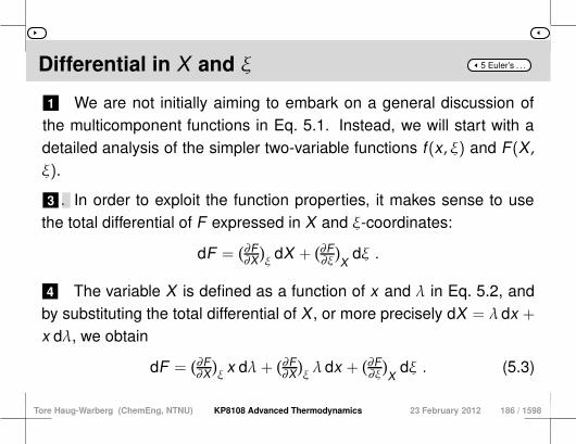
5 Euler’s . . .Differential in X and ξ
1 We are not initially aiming to embark on a general discussion ofthe multicomponent functions in Eq. 5.1. Instead, we will start with adetailed analysis of the simpler two-variable functions f(x, ξ) and F(X ,ξ).
3 2 The results will later be generalised in Chapter General Theory,and we lose nothing by taking an easy approach here. In order to exploit the function properties, it makes sense to use
the total differential of F expressed in X and ξ-coordinates:
dF =(∂F∂X
)ξ
dX +(∂F∂ξ
)X
dξ .
4 The variable X is defined as a function of x and λ in Eq. 5.2, andby substituting the total differential of X , or more precisely dX = λdx +
x dλ, we obtain
dF =(∂F∂X
)ξ
x dλ+(∂F∂X
)ξλdx +
(∂F∂ξ
)X
dξ . (5.3)
Tore Haug-Warberg (ChemEng, NTNU) KP8108 Advanced Thermodynamics 23 February 2012 186 / 1598
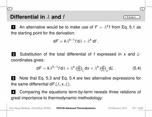
5 Euler’s . . .Differential in λ and f
1 An alternative would be to make use of F = λk f from Eq. 5.1 asthe starting point for the derivation:
dF = kλk−1f dλ+ λk df .
2 Substitution of the total differential of f expressed in x and ξ-coordinates gives:
dF = kλk−1f dλ+ λk (∂f∂x
)ξ
dx + λk (∂f∂ξ
)x
dξ . (5.4)
3 Note that Eq. 5.3 and Eq. 5.4 are two alternative expressions forthe same differential dF (λ, x, ξ).
4 Comparing the equations term-by-term reveals three relations ofgreat importance to thermodynamic methodology:
Tore Haug-Warberg (ChemEng, NTNU) KP8108 Advanced Thermodynamics 23 February 2012 187 / 1598

5 Euler’s . . .Case dλ
1 Comparing the dλ terms reveals that (∂F/∂X)ξ x = kλk−1f . Mul-tiplying both sides by λ gives (∂F/∂X)ξ λx = kλk f , which if we substi-tute in Eq. 5.1 and Definition 5.2 can be transformed into:
(∂F∂X
)ξ
X = kF . (5.5)
3 2 The closed form of Eq. 5.5 indicates that there is a general solutionto the indefinite integral F(X , ξ) =
∫(dF)ξ =
∫(∂F/∂X)ξ dX . The result is known as Euler6s first theorem for homogeneous func-
tions, or simply as the Euler integration of F .
6 Leonhard Euler, 1707–1783. Swiss mathematician.
Tore Haug-Warberg (ChemEng, NTNU) KP8108 Advanced Thermodynamics 23 February 2012 188 / 1598

5 Euler’s . . .Case dx
1 Comparing the dx terms reveals that (∂F/∂X)ξ λ = λk (∂f/∂x)ξ.Dividing each side by λ leads to:
(∂F∂X
)ξ= λk−1 (∂f
∂x)ξ. (5.6)
3 2 Because F has the same function definition as f (it is only thenames of the free variables that differ) it follows that ∂F/∂X and ∂f/∂xare equivalent functions. Hence, (∂F/∂X)ξ is a homogeneous function of order k − 1.
4 Differentiation with respect to X therefore reduces the order of ho-mogeneity of F by one.
Tore Haug-Warberg (ChemEng, NTNU) KP8108 Advanced Thermodynamics 23 February 2012 189 / 1598

5 Euler’s . . .Case dξ
1 Comparing the dξ-terms reveals that the homogeneity of thederivative with respect to ξ is unchanged:
(∂F∂ξ
)X= λk (∂f
∂ξ
)x, (5.7)
3 2 Using the same arguments as in the case above this implies thatthe derivative of F with respect to ξ is a new homogeneous function ofdegree k . Differentiation with respect to ξ therefore conserves the homogene-
ity in X .
Tore Haug-Warberg (ChemEng, NTNU) KP8108 Advanced Thermodynamics 23 February 2012 190 / 1598

5 Euler’s . . .Note
1 It should be stressed that the Euler integration in Eq. 5.5 is notlimited to one particular interpretation of X .
2 In fact, any scaled variable x = λ-1X satisfies the equation:(∂f∂x
)ξ
x = kf .
3 The validity of this statement is confirmed by first combiningEqs. 5.5 and 5.6, and then substituting in Eq. 5.1 and Definition 5.2.4 This result emphasises the practical importance of Euler’s theorem
as outlined in Eq. 5.5.
Tore Haug-Warberg (ChemEng, NTNU) KP8108 Advanced Thermodynamics 23 February 2012 191 / 1598
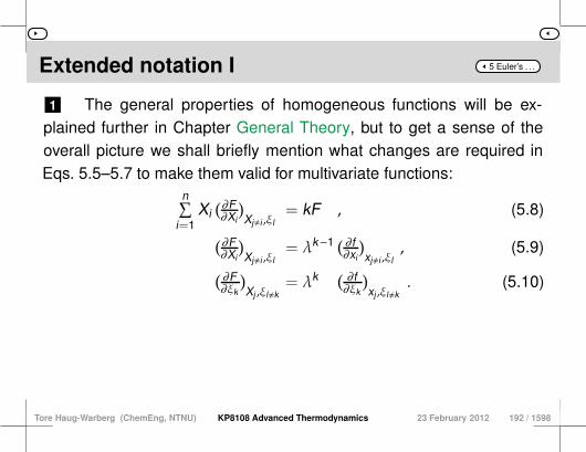
5 Euler’s . . .Extended notation I
1 The general properties of homogeneous functions will be ex-plained further in Chapter General Theory, but to get a sense of theoverall picture we shall briefly mention what changes are required inEqs. 5.5–5.7 to make them valid for multivariate functions:
n∑i=1
Xi(∂F∂Xi
)Xj,i ,ξl
= kF , (5.8)
(∂F∂Xi
)Xj,i ,ξl
= λk−1 ( ∂f∂xi
)xj,i ,ξl
, (5.9)( ∂F∂ξk
)Xj ,ξl,k
= λk ( ∂f∂ξk
)xj ,ξl,k
. (5.10)
Tore Haug-Warberg (ChemEng, NTNU) KP8108 Advanced Thermodynamics 23 February 2012 192 / 1598
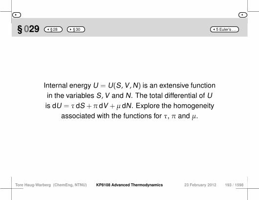
5 Euler’s . . .§ 029 § 28 § 30
Internal energy U = U(S ,V ,N) is an extensive functionin the variables S ,V and N. The total differential of Uis dU = τdS +πdV +µ dN. Explore the homogeneity
associated with the functions for τ, π and µ.
Tore Haug-Warberg (ChemEng, NTNU) KP8108 Advanced Thermodynamics 23 February 2012 193 / 1598
5 Euler’s . . .§ 029 Intensive functions
1 The variables τ, π and µ mentioned above must first be defined.Mathematically, the total differential of U(S ,V ,N) is:
dU =(∂U∂S
)V ,N dS +
(∂U∂V
)S,N dV +
(∂U∂N
)S,V dN .
3 2 Comparing this with the differential given in the text implies thatτ = (∂U/∂S)V ,N, π = (∂U/∂V)S,N and µ = (∂U/∂N)S,V , see also Para-graph 19 on page 117 in Chapter 4. Substitution of k = 1, Xi = S, Xj ∈ V ,N and ξl = ∅
7 in Eq. 5.9yields:
τ(S ,V ,N) =(∂U(S,V ,N)
∂S)V ,N = λ0 (∂u(s,v,n)
∂s)v,n = τ(s, v, n) . (5.11)
4 The function τ(S ,V ,N) is obviously homogeneous of order 0 in thevariables S ,V ,N because it is independent of the scaling factor λ.
Tore Haug-Warberg (ChemEng, NTNU) KP8108 Advanced Thermodynamics 23 February 2012 194 / 1598
5 Euler’s . . .§ 029 Intensive functions (2)
6 5 The temperature is commonly referred to as an intensive variableand is taken to be independent of the system sizea.
a Valid only when the system is sufficiently big i.e. when the number of particles is largeenough to fix the temperature. Similarly, differentiation of U with respect to V and N yields
π(S ,V ,N) =(∂U(S,V ,N)
∂V)S,N = λ0 (∂u(s,v,n)
∂v)s,n = π(s, v, n) , (5.12)
µ(S ,V ,N) =(∂U(S,V ,N)
∂N)S,V = λ0 (∂u(s,v,n)
∂n)s,v = µ(s, v, n) , (5.13)
where the (negative) pressure and the chemical potential are intensivevariables as well.
7 Actually an empty set. Here it is used to denote a missing variable or an emptyvector.
Tore Haug-Warberg (ChemEng, NTNU) KP8108 Advanced Thermodynamics 23 February 2012 195 / 1598

5 Euler’s . . .§ 030 § 29 § 31
Internal energy U = U(S ,V ,N) is an extensive functionin the variables S ,V and N. The total differential ofU is dU = τdS + πdV + µ dN. What is the correct
integral form of U? Explain the physical significanceof this integral.
Tore Haug-Warberg (ChemEng, NTNU) KP8108 Advanced Thermodynamics 23 February 2012 196 / 1598
5 Euler’s . . .§ 030 Euler integration
1 Substituting k = 1, Xi ∈ S ,V ,N and ξl = ∅ into Eq. 5.8, togetherwith the definitions from Paragraph 29 on page 182 i.e. τ = (∂U/∂S)V ,N,π = (∂U/∂V)S,N and µ = (∂U/∂N)S,V yields Euler’s equation applied tointernal energy:
U = τS + πV + µN . (5.14)
2 We are not being asked about multicomponent mixtures, butEq. 5.14 is quite general and can (by analogy with Eq. 5.8) be extendedto:
U = τS + πV +n∑
i=1µiNi = τS + πV + µTn (5.15)
Tore Haug-Warberg (ChemEng, NTNU) KP8108 Advanced Thermodynamics 23 February 2012 197 / 1598
5 Euler’s . . .Remark
1 The total differential of internal energy for a single componentsystem is dU = τdS + πdV + µ dN.
3 2 The differential can be integrated without actually solving anypartial differential equations because τ, π, µ are intensive (size-independent) variables. Physically, this means that the system can be built up from zero
size8 in a manner that keeps τ, π, µ constant during the process.
5 4 This is achieved by combining a large number of small systems atfixed temperature, (negative) pressure and chemical potential. When these subsystems are merged into one big system there will
be no changes in the intensive properties, because the requirements forthermodynamic equilibrium are automatically fulfilled, see also Chap-ter 21 on page 1162.
8 By definition, a system of zero size has zero internal energy, i.e. U = 0. In thiscontext, “zero size” refers to zero volume, zero mass and zero entropy. Note, however,that it is not sufficient to assume zero mass, because even an evacuated volume willhave radiation energy proportional to T 4!
Tore Haug-Warberg (ChemEng, NTNU) KP8108 Advanced Thermodynamics 23 February 2012 198 / 1598

5 Euler’s . . .§ 031 § 30 § 32
Gibbs energy G(τ, π,N) is an extensive function ofthe mole number N at a given temperature τ and(negative) pressure π. The total differential of G is
dG = −S dτ−V dπ+µ dN. Explore the homogeneityassociated with the functions S and V .
Tore Haug-Warberg (ChemEng, NTNU) KP8108 Advanced Thermodynamics 23 February 2012 199 / 1598

5 Euler’s . . .§ 031 Extensive functions
1 2 We will apply the same procedure as was used in Paragraph 29 onpage 182. First of all the functions S ,V and µ must be defined. Mathemati-
cally, the total differential of G(τ, π,N) is:
dG =(∂G∂τ
)π,N dτ+
(∂G∂π
)τ,N dπ+
(∂G∂N
)τ,π
dN .
3 Comparing this with the differential in the problem formulationyields −S(τ, π,N) = (∂G/∂τ)π,N , −V(τ, π,N) = (∂G/∂π)τ,N and µ =
(∂G/∂N)τ,π.
5 4 From Eq. 5.10 we can deduce that both volume and entropy arehomogeneous functions of order 1 in the mole number at specified tem-perature and (negative) pressure, i.e. they are extensive variables. From Eq. 5.9 it can be seen that the chemical potential is (still) a
homogeneous function of order 0, see also Eq. 5.13.
Tore Haug-Warberg (ChemEng, NTNU) KP8108 Advanced Thermodynamics 23 February 2012 200 / 1598
5 Euler’s . . .§ 032 § 31 § 33Non-canonical variables1 Any further discussion of homogeneity should ideally be based on
the properly identified canonical state variables of the function.
2 However, this is not an absolute condition, as the thermodynamicstate of a system is uniquely determined when any of its independentvariable sets is fully specified.
3 For example U is extensive in S ,V ,N while G is extensive in N at agiven τ and π, but we can alternatively state the opposite and say thatU is extensive in N at a given τ and π and that G is extensive in S ,V ,N.
4 There are plenty of alternative ways to describe the system, but acombination of three arbitrary state variables is not always sufficient.
5 To demonstrate this, let us look at the specification H, τ,N.
6 For example, the ideal gas enthalpy can be written Hıg = H(τ,N).At a given τ,N the system is underspecified, because there is no waywe can determine the pressure.
7 If we try to specify H in addition to τ and N, this will give us aredundant (or even contradictory) statement.
8 To avoid problems of this kind we shall therefore make use ofcanonical variables unless otherwise stated.
201 / 1598
The Gibbs energy of a binary mixture is given as ahomogeneous function of order 1 in the mole numbersN1 and N2 (at fixed T and p). Make a contour diagram
illustrating the function G = aN1x2+N1 ln x1+N2lnx2 whereN2 is plotted along the ordinate axis and N1 along the
abscissa. Let x1 = N1/(N1 +N2) and x2 = N2/(N1 +N2).Show that the isopleths corresponding to constantG (the contour lines) are equidistant for a series of
evenly distributed Gibbs energy values. Use a = 2.4in your calculations.
Tore Haug-Warberg (ChemEng, NTNU) KP8108 Advanced Thermodynamics 23 February 2012 202 / 1598
5 Euler’s . . .§ 032 Gibbs energy I
1 The function is nonlinear in N1 and N2, and the isopleths must becalculated iteratively using e.g. Newton–Raphson’s method: N2,k+1 =
N2,k − (Gk −G)/µ2, where µ2 = ax21 + ln x2 is the partial derivative of G
with respect to N2.
2 A fixed value is selected for N1, and N2 is iterated until Gk→∞ hasconverged to G, see the Matlab-program 1.4 in Appendix 30.
4 3 The result obtained is shown in Figure 5.1 on page 193. Note that each isopleth defines a non-convex region, which can beinterpreted as a fundamental thermodynamic instability.
Tore Haug-Warberg (ChemEng, NTNU) KP8108 Advanced Thermodynamics 23 February 2012 203 / 1598

5 Euler’s . . .§ 032 Gibbs energy I (2)
5 The corresponding two-phase region (the symmetry of the modelreduces the phase equilibrium criterion to µ1 = µ2) can be calculatedfrom the total differential of G, rewritten here into the tangent of theisopleth:
(dN2dN1
)T ,p,G
= − µ1µ2.
7 6 It can be proved (do it!) that the tangent intersects with the y and xaxes at G/µ2 and G/µ1 respectively. This indicates that the phase equilibrium condition is fulfilled when-
ever two points on the same isopleth have common tangents (remem-ber that G takes constant values along each isopleth such that the cri-terion is reduced to µ1 = µ2).
Tore Haug-Warberg (ChemEng, NTNU) KP8108 Advanced Thermodynamics 23 February 2012 204 / 1598
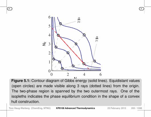
0 2 4 60
1
2
3
4
5
6
N1
N2
Gµ1
Gµ2
Figure 5.1: Contour diagram of Gibbs energy (solid lines). Equidistant values(open circles) are made visible along 3 rays (dotted lines) from the origin.The two-phase region is spanned by the two outermost rays. One of theisopleths indicates the phase equilibrium condition in the shape of a convexhull construction.
Tore Haug-Warberg (ChemEng, NTNU) KP8108 Advanced Thermodynamics 23 February 2012 205 / 1598
5 Euler’s . . .§ 033 § 32 § 34
Homogeneity causes a whole range of remarkableresults. One formula obtained by differentiating Eq. 5.5
is:
X d(∂F∂X
)ξ− k
(∂F∂ξ
)X
dξ = (k − 1)(∂F∂X
)ξ
dX ,
For k = 1 this implies that (∂2F/∂X∂X)ξ = 0 and(∂F/∂ξ)X = (∂2F/∂X∂ξ)X . Verify these results and
give a physical explanation for them.
Tore Haug-Warberg (ChemEng, NTNU) KP8108 Advanced Thermodynamics 23 February 2012 206 / 1598
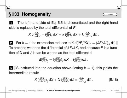
5 Euler’s . . .§ 033 Homogeneity
1 The left-hand side of Eq. 5.5 is differentiated and the right-handside is replaced by the total differential of F :
X d(∂F∂X
)ξ+
(∂F∂X
)ξ
dX = k(∂F∂X
)ξ
dX + k(∂F∂ξ
)X
dξ .
2 For k = 1 the expression reduces to X d(∂F/∂X)ξ = (∂F/∂ξ)X dξ. 3 Note that X and dξ are arbitrary.
To proceed we need the differential of ∂F/∂X , and because F is a func-tion of X and ξ it can be written as the total differential
d(∂F∂X
)ξ=
( ∂2F∂X∂X
)ξ
dX +( ∂2F∂X∂ξ
)dξ ,
5 4 where dX is also arbitrary. Substituted into the equation above (letting k = 1), this yields theintermediate result:
X( ∂2F∂X∂X
)ξ
dX + X( ∂2F∂X∂ξ
)dξ =
(∂F∂ξ
)X
dξ . (5.16)
Tore Haug-Warberg (ChemEng, NTNU) KP8108 Advanced Thermodynamics 23 February 2012 207 / 1598

5 Euler’s . . .§ 033 Homogeneity (2)
7 6 The trick is to recognise that X , dX and dξ are independent vari-ables. This implies that two non-trivial relations follow from Eq. 5.16 (one
equation in three variables gives two non-trivial relations), irrespectiveof the actual values of X , dX , ξ and dξ:
( ∂2F∂X∂X
)ξ= 0 , (5.17)
X( ∂2F∂X∂ξ
)=
(∂F∂ξ
)X
(5.18)
Tore Haug-Warberg (ChemEng, NTNU) KP8108 Advanced Thermodynamics 23 February 2012 208 / 1598

5 Euler’s . . .Parametric form
1 From a physical point of view any extensive function F(X , ξ) canbe expressed in the form F = β(ξ)X .
2 This stems from the fact that F(0, ξ) = 0 in addition to ∂2F/∂X∂X =
0, see Eq. 5.179 The derivative of F with respect to ξ is therefore anextensive function β′(ξ)X where the second derivative of F with respectto both X and ξ is equal to the intensive parameter β′(ξ).3 The numerical value of ∂F/∂ξ can easily be obtained by integrating
∂2F/∂X∂ξ using the Euler method as shown in Eq. 5.18.
9 It should be noted that it is the second derivative function which is zero. It is notsufficient to say that the second derivative is zero at a given point.
Tore Haug-Warberg (ChemEng, NTNU) KP8108 Advanced Thermodynamics 23 February 2012 209 / 1598
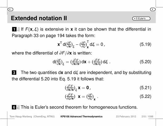
5 Euler’s . . .Extended notation II
1 2 In the general case, x and ξ would be vector quantities. If F(x, ξ) is extensive in x it can be shown that the differential inParagraph 33 on page 194 takes the form:
xT d(∂F∂x
)ξ− (∂F
∂ξ
)T
xdξ = 0 , (5.19)
where the differential of ∂F/∂x is written:
d(∂F∂x
)ξ=
( ∂2F∂x∂x
)dx +
( ∂2F∂x∂ξ
)dξ . (5.20)
3 The two quantities dx and dξ are independent, and by substitutingthe differential 5.20 into Eq. 5.19 it follows that:
( ∂2F∂x∂x
)ξ
x = 0 , (5.21)( ∂2F∂ξ∂x
)x =
(∂F∂ξ
)x. (5.22)
6 4 From a logical point of view Eq. 5.22 is a true generalisation of 5.18,whereas Eq. 5.17 represents a specialisation of 5.21.5 This means that the second derivative of F(X , ξ) with respect to X
is zero for all single-variable functions, while the corresponding HessianF(x, ξ) for multivariate systems is singular in the direction of x, where x
is proportional to one of the eigenvectors of the Hessian. This is Euler’s second theorem for homogeneous functions.
Tore Haug-Warberg (ChemEng, NTNU) KP8108 Advanced Thermodynamics 23 February 2012 210 / 1598
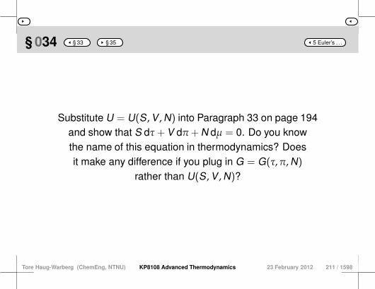
5 Euler’s . . .§ 034 § 33 § 35
Substitute U = U(S ,V ,N) into Paragraph 33 on page 194and show that S dτ+V dπ+N dµ = 0. Do you knowthe name of this equation in thermodynamics? Doesit make any difference if you plug in G = G(τ, π,N)
rather than U(S ,V ,N)?
Tore Haug-Warberg (ChemEng, NTNU) KP8108 Advanced Thermodynamics 23 February 2012 211 / 1598

5 Euler’s . . .§ 034 Gibbs–Duhem
1 Substituting F = U(x, ξ) into Eq. 5.19 where xT = (S ,V ,N) andξ = ∅, reduces the expression to xT d(∂U/∂x) = 0. From the definitionsof τ, π and µ in Paragraph 29 on page 182 we can write
S dτ+ V dπ+ N dµ = 0 , (5.23)
3 2 which is better known as the Gibbs–Duhem equation. Alternatively, if F = G(x, ξ) where x = N and ξT = (τ, π), thenEq. 5.19 takes the form:
N d(∂G∂N
)τ,π− (∂G
∂τ
)π,N dτ − (∂G
∂π
)τ,N dπ = 0 .
4 The partial derivatives of G with respect to N, τ and π have beenidentified as µ,−S and −V in Paragraph 31 on page 188.
5 The expression can therefore be reformulated as N dµ + S dτ +
V dπ = 0 which is identical to the Gibbs–Duhem equation.
Tore Haug-Warberg (ChemEng, NTNU) KP8108 Advanced Thermodynamics 23 February 2012 212 / 1598
5 Euler’s . . .§ 034 Gibbs–Duhem (2)
6 In fact, all Legendre transforms of U end up giving the same Gibbs–Duhem equation.
Tore Haug-Warberg (ChemEng, NTNU) KP8108 Advanced Thermodynamics 23 February 2012 213 / 1598

5 Euler’s . . .Comment
1 We have not been asked for any extensions, but by analogy toEqs. 5.8 and 5.15 the Gibbs–Duhem equation may be extended to amulticomponent form:
S dτ+ V dπ+n∑
i=1Ni dµi = S dτ+ V dπ+ nT dµ = 0 . (5.24)
4 2 Note that the Gibbs–Duhem equation follows inevitably from theproperties of extensive functions when differentiated, which in turn re-flect their homogeneity.3 This is true for all functions of this kind, and not only thermody-
namic ones. The homogeneity, which effectively removes one degree of free-dom in the function expression, shows up as a mutual dependency inthe nth derivatives (of U).
6 5 As a result, only n − 1 of the intensive state variables are indepen-dent. In single component systems this means that any arbitrary inten-
sive variable can be expressed as a function of (at most) two other in-tensive variables, see also Paragraph 39 on page 214.
Tore Haug-Warberg (ChemEng, NTNU) KP8108 Advanced Thermodynamics 23 February 2012 214 / 1598
5 Euler’s . . .
1 It is important to realise that the information contained in U is con-served during the Legendre transformation to H,A , . . . ,O .
2 For example, knowing the Gibbs energy G(τ, π,N) really impliesfull knowledge of U(S ,V ,N), and vice versa.
3 The Gibbs–Duhem equation can therefore be derived from any ofthe energy functions.
4 In particular this also applies to the differential of the null-potentialO(τ, π, µ) which is identical to Eq. 5.23, see Paragraph 26 on page 157.
Tore Haug-Warberg (ChemEng, NTNU) KP8108 Advanced Thermodynamics 23 February 2012 215 / 1598

5 Euler’s . . .§ 035 § 34 § 36
Use the result from Paragraph 33 on page 194 todetermine the second derivatives (∂2G/∂N∂N)τ,π,
(∂2Y/∂S∂S)π,µ and (∂2Ω/∂V∂V)τ,µ, where G = G(τ,
π,N) and Y = Y(S , π, µ) and Ω = Ω(τ,V , µ).
Tore Haug-Warberg (ChemEng, NTNU) KP8108 Advanced Thermodynamics 23 February 2012 216 / 1598

5 Euler’s . . .§ 035 Linear potentials
1 The three functions G,Y and Ω are extensive in N,S and V re-spectively, i.e. in one variable each.
2 This makes Eq. 5.17 valid and the substitution of the definitions forτ, π and µ yields:
( ∂2G∂N∂N
)τ,π
=(∂µ∂N
)τ,π
= 0 , (5.25)( ∂2Y∂S∂S
)π,µ
=(∂τ∂S
)π,µ
= 0 , (5.26)( ∂2Ω∂V∂V
)τ,µ
=(∂π∂V
)τ,µ
= 0 . (5.27)
Tore Haug-Warberg (ChemEng, NTNU) KP8108 Advanced Thermodynamics 23 February 2012 217 / 1598
5 Euler’s . . .§ 036 § 35 § 37
Show that the Hessian of A = A(τ,V ,N) has onlyone independent element when the temperature τ istaken to be a constant parameter. Use Eq. 5.21 as
your starting point.
Tore Haug-Warberg (ChemEng, NTNU) KP8108 Advanced Thermodynamics 23 February 2012 218 / 1598

5 Euler’s . . .Example
1 Helmholtz energy is extensive in V ,N at any given temperature τ.
2 Bearing in mind Eq. 5.21 the Hessian of A can be expressed as afunction of only one independent variable because the matrix, in addi-tion to being symmetric, must satisfy the relation:
( ∂2A∂x∂x
)τ
x =
(∂π∂V
)τ,N
(∂π∂N
)τ,V
(∂µ∂V
)τ,N
(∂µ∂N
)τ,V
V
N
=
0
0
.
3 The fact that the matrix, like all Hessians, must be symmetric, inthis case leads to (∂π/∂N)τ,V = (∂µ/∂V)τ,N.
4 Altogether there are 4 matrix elements, with 3 associated relations.
Tore Haug-Warberg (ChemEng, NTNU) KP8108 Advanced Thermodynamics 23 February 2012 219 / 1598

5 Euler’s . . .§ 036 Hessians
1 The solution of the homogeneous (!) system of equations can beformulated in an infinite number of ways, one of which is:
NV
(∂µ∂N
)τ,V
NV −1−1 V
N
VN
=
00
. (5.28)
2 Note that the second derivative of Helmholtz energy with respectto the mole number is non-zero in Eq. 5.28, while the correspondingsecond derivative of Gibbs energy is zero in Eq. 5.25:
fra 5.25:(∂µ∂N
)τ,π
= 0 ,
og fra 5.28:(∂µ∂N
)τ,V , 0 .
3 This emphasises the fact that it is important to have a proper un-derstanding of the many peculiarities of the energy functions, and it alsohighlights that it is essential to know which variables are held constantduring differentiation.
Tore Haug-Warberg (ChemEng, NTNU) KP8108 Advanced Thermodynamics 23 February 2012 220 / 1598

5 Euler’s . . .§ 037 § 36 § 38
Find analytical expressions for (∂G/∂τ)π,N and (∂G/∂π)τ,Nby using the Euler method to integrate the partial molar
entropy and partial molar volume.
Tore Haug-Warberg (ChemEng, NTNU) KP8108 Advanced Thermodynamics 23 February 2012 221 / 1598

5 Euler’s . . .§ 037 Partial molarity
1 Replace F by G(ξ,n) in Eq. 5.22, where ξT = (τ, π) and nT =
(N1, . . . ,Nn). This gives, without much difficulty:
(∂G∂τ
)π,N
(∂G∂π
)τ,N
=
( ∂2G∂τ∂nT
)π
( ∂2G∂π∂nT
)τ
n = −
( ∂S∂nT
)τ,π
( ∂V∂nT
)τ,π
n = −
sTn
vTn
.
2 The partial derivatives of S and V on the right hand side are calledthe partial molar entropy and partial molar10 volume respectively.
4 3 These and other partial molar quantities occur so frequently in thethermodynamic theory of mixtures that they have been given their owndifferential operator, see Paragraph 10 on page 76. A more compact notation is therefore S = nTs and V = nTv.
10 A partial molar quantity is defined as f = (∂F/∂n)τ,π, irrespective of whether or notF has τ,π,N1, . . . ,Nn as canonical variables (it is only for Gibbs energy that there is acorrespondence between the two sets of variables).
Tore Haug-Warberg (ChemEng, NTNU) KP8108 Advanced Thermodynamics 23 February 2012 222 / 1598

5 Euler’s . . .§ 038 § 37 § 39
Show that G(S ,V ,N) is really an extensive function ofthe variables S ,V and N, thus verifying the conjecture
set out in the introduction to this chapter (on page 190).
Tore Haug-Warberg (ChemEng, NTNU) KP8108 Advanced Thermodynamics 23 February 2012 223 / 1598
5 Euler’s . . .§ 038 Proof
1 From the definition G(τ, π,N) = U − τS − πV , where U = U(S ,V ,N), τ = (∂U/∂S)V ,N and π = (∂U/∂V)S,N, it follows that we can expressGibbs energy as a function of S ,V and N, because the right-hand sideof the equation only includes U and functions derived from U:
G(S ,V ,N) = U(S ,V ,N) − τ(S ,V ,N)S − π(S ,V ,N)V .
2 We already know that τ and π are intensive variables, whereasU,S and V are extensive variables.
Tore Haug-Warberg (ChemEng, NTNU) KP8108 Advanced Thermodynamics 23 February 2012 224 / 1598

5 Euler’s . . .§ 038 Proof (2)
3 From this it follows that
G(S ,V ,N) = λu(s, v, n) − λτ(s, v, n)s − λπ(s, v, n)v= λg(s, v, n) ,
which clearly demonstrates that G is homogeneous, in accordance withthe conjecture.4 Note that the last equation tacitly assumes the homogeneity rela-
tions S = λs,V = λv and N = λn.
Tore Haug-Warberg (ChemEng, NTNU) KP8108 Advanced Thermodynamics 23 February 2012 225 / 1598
5 Euler’s . . .§ 039 § 38 § 40
Starting from Paragraph 35 on page 204, can you tellhow many thermodynamic variables are needed to
determine the intensive state of a system?
Tore Haug-Warberg (ChemEng, NTNU) KP8108 Advanced Thermodynamics 23 February 2012 226 / 1598

5 Euler’s . . .§ 039 The state concept
1 A thermodynamic system is normally described by n + 2 indepen-dent state variables.
2 However, the intensive state can be determined once n + 1 (inten-sive) variables are known.
4 3 This fact is illustrated by Eqs. 5.25–5.27, where the derivative ofan intensive property with respect to an extensive variable is zero if theother variables are intensive, and are held constant during differentia-tion. In fact, the (single) extensive variable determines the system size
but has no influence on τ, π and µ.
5 For a single-component system we can describe the intensive statein three different ways:
τ = τ(π, µ) ,
π = π(τ, µ) ,
µ = µ(τ, π) .
Tore Haug-Warberg (ChemEng, NTNU) KP8108 Advanced Thermodynamics 23 February 2012 227 / 1598

Ideal gas law Molecules Photons Phonons Free electrons Virial Van der Waals Murnaghan
Part 7
Equations of state
see also Part-Contents
Tore Haug-Warberg (ChemEng, NTNU) KP8108 Advanced Thermodynamics 23 February 2012 252 / 1598

Ideal gas law Molecules Photons Phonons Free electrons Virial Van der Waals Murnaghan
Contents
1 Ideal gas law
1 Helmholtz potential2 Gibbs potential3 Grand canonical potential
2 Molecules
1 Translation2 Vibration3 Rotation4 Other intra-molecular degrees of freedom
3 Photons
4 Phonons
5 Free electrons
Tore Haug-Warberg (ChemEng, NTNU) KP8108 Advanced Thermodynamics 23 February 2012 253 / 1598
Ideal gas law Molecules Photons Phonons Free electrons Virial Van der Waals Murnaghan
Contents (2)
6 Virial
7 Van der Waals
8 Murnaghan
Tore Haug-Warberg (ChemEng, NTNU) KP8108 Advanced Thermodynamics 23 February 2012 254 / 1598

Ideal gas law Molecules Photons Phonons Free electrons Virial Van der Waals Murnaghan
7 Equations . . .State description
1 Although thermodynamics builds on some basic, fundamentalprinciples of physical science, which form part of a well-defined mathe-matical theory, it is essentially an empirical science.
3 2 This is particularly true of the many semi-empirical models that areused in engineering research. That is how it was in the past, and that is how it will continue to be
in the future, because with the exception of a handful of simplificationsused in statistical mechanics1 there are no precise models, and therewill always be the need for essentially physical models with adjustableparameters.
6 4 A thermodynamic state description needs one or more functions ofstate that define the asymptotes of the system (mixture) in a consistentmanner.5 Applying parameters to the functions gives engineers the flexibility
they need, while it also ensures thermodynamic consistency. In this chapter we learn about a variety of useful concepts, such asideal gases, virial development, the Einstein–Debye phonon model andvan der Waals theory, but first of all we need to define the concept of anequation of state.
Tore Haug-Warberg (ChemEng, NTNU) KP8108 Advanced Thermodynamics 23 February 2012 255 / 1598

Ideal gas law Molecules Photons Phonons Free electrons Virial Van der Waals Murnaghan
7 Equations . . .State description (2)
7 Let us start with any canonical differential, e.g. of internal energy
dU = T dS − p dV +n∑
i=1µi dNi , (7.1)
defined using the canonical variables S ,V ,Ni.
8 If we know the fundamental state functions referred to as the equa-tions of state of the system
T = T(S ,V ,n) , (7.2)
p = p(S ,V ,n) , (7.3)
µi = µi(S ,V ,n) , (7.4)
then Eq. 7.1 can be integrated using Euler’s 1st theorem to give U =
TS − pV +∑n
i=1 µiNi, as shown in Paragraph 30 in Chapter 5. However,
Tore Haug-Warberg (ChemEng, NTNU) KP8108 Advanced Thermodynamics 23 February 2012 256 / 1598
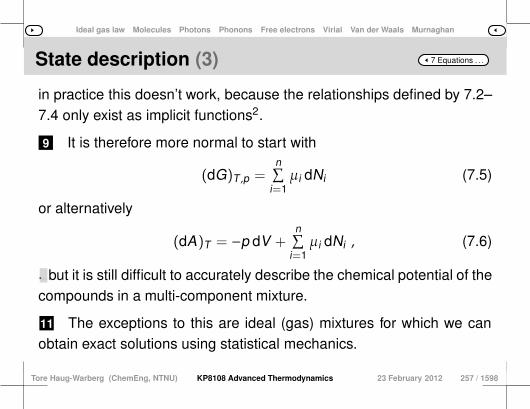
Ideal gas law Molecules Photons Phonons Free electrons Virial Van der Waals Murnaghan
7 Equations . . .State description (3)
in practice this doesn’t work, because the relationships defined by 7.2–7.4 only exist as implicit functions2.
9 It is therefore more normal to start with
(dG)T ,p =n∑
i=1µi dNi (7.5)
or alternatively
(dA)T = −p dV +n∑
i=1µi dNi , (7.6)
10 which can be integrated in the same way if the state function(s)µi(T , p,n) or p(T ,V ,n) and µi(T ,V ,n) are known,a
a Many textbooks refer to p(T ,V ,n) as if there were no other state functions, but thatis wrong! but it is still difficult to accurately describe the chemical potential of thecompounds in a multi-component mixture.
11 The exceptions to this are ideal (gas) mixtures for which we canobtain exact solutions using statistical mechanics.
Tore Haug-Warberg (ChemEng, NTNU) KP8108 Advanced Thermodynamics 23 February 2012 257 / 1598
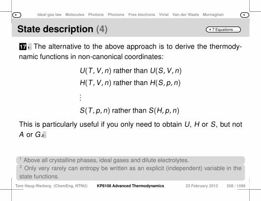
Ideal gas law Molecules Photons Phonons Free electrons Virial Van der Waals Murnaghan
7 Equations . . .State description (4)
17 12 By taking the ideal gas model as a reference, it is relatively easy toobtain the residual functions Gr,p(T , p,n) =
∫(V(T , p,n)− V ıg)dp
13 or A r,v(T ,V ,n) =∫(p(T ,V ,n) − pıg)dV ,
14 which describe the difference between a real mixture and an equiv-alent ideal gas under the same physical conditions.15 If we combine this with an expression for the energy of the refer-ence gas, we get the Gibbs or Helmholtz energy of the mixture, and afull set of state functions can then be derived using differentiation.16 This leaves us with just V(T , p,n) or p(T ,V ,n) as the state func-tions. The alternative to the above approach is to derive the thermody-
namic functions in non-canonical coordinates:
U(T ,V , n) rather than U(S ,V , n)
H(T ,V , n) rather than H(S , p, n)...
S(T , p, n) rather than S(H, p, n)
This is particularly useful if you only need to obtain U, H or S, but notA or G.18 Typically, this is the case for physical state changes that occur at a
constant composition like for instance fluid flow in pipes, compressorsand valves.19 For systems of variable composition, where the chemical poten-tial is important, it is more suitable to use A and G because µi =
(∂A/∂Ni)T ,V ,Nj,i = (∂G/∂Ni)T ,p,Nj,i
20 can be obtained later using differentiation with respect to thecanonical variables.21 If we choose to disregard canonical theory for a moment, thenthe chemical potential must be defined as µi = (∂H/∂Ni)T ,p,Nj,i −T (∂S/∂Ni)T ,p,Nj,i = hi − Tsi
22 or a similar expression based on U, but this approach normallyinvolves more work.
1 Above all crystalline phases, ideal gases and dilute electrolytes.2 Only very rarely can entropy be written as an explicit (independent) variable in thestate functions.
Tore Haug-Warberg (ChemEng, NTNU) KP8108 Advanced Thermodynamics 23 February 2012 258 / 1598

Ideal gas law Molecules Photons Phonons Free electrons Virial Van der Waals Murnaghan
7 Equations . . .Ideell (perfect) gas
1 2 The term ideal (perfect) gas refers to ideal, and from a physicalpoint of view hypothetical, descriptions of the conditions in a real gas. An ideal gas consists of individual particles (atoms, molecules or
radicals) that move freely and independently in space, without any kindof interaction.
5 3 This is the ideal situation because it involves ignoring the inter-molecular forces that exist between the particles in a real gas.4 This includes all of the interactions caused by induced dipoles (van
der Waals forces), dipole-dipole forces, dipole-quadrupole forces, etc. In spite of this massive simplification, the total energy of the gas isnot equal to zero, as the particles have their kinetic energy (translation),moment of inertia (rotation), internal degrees if freedom (vibration, in-ternal rotation, torsion, electronic excitation) and chemical binding en-ergy.
7 6 Furthermore, electron and nuclear spin can also play a role. Ideal gases are only valid as a special case of the true thermody-namic state when pressure approaches zero, and can never be mea-sured directly in a real (physical) system.8 Nevertheless, we must be allowed to consider the ideal gas law
one of the great scientific discoveries.9 Perhaps it is just as important as Maxwell’s equations, which de-
scribe electromagnetism, although that is a very subjective judgement,as Maxwell’s equations are a complex set of four linked partial differ-ential equations, whereas the ideal gas law is just a simple algebraicequation.10 What they have in common, then, is not their mathematical formu-lae, but rather their understanding of the underlying physics and of thepractical and theoretical implications.
Tore Haug-Warberg (ChemEng, NTNU) KP8108 Advanced Thermodynamics 23 February 2012 259 / 1598
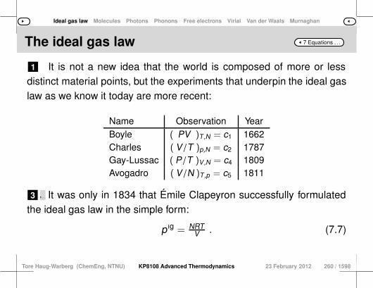
Ideal gas law Molecules Photons Phonons Free electrons Virial Van der Waals Murnaghan
7 Equations . . .The ideal gas law
1 It is not a new idea that the world is composed of more or lessdistinct material points, but the experiments that underpin the ideal gaslaw as we know it today are more recent:
Name Observation YearBoyle ( PV )T ,N = c1 1662Charles ( V/T )p,N = c2 1787Gay-Lussac ( P/T )V ,N = c4 1809Avogadro (V/N )T ,p = c5 1811
3 2 Given what we know today, the above table accurately representsthe scientific progress, but at the time the scientists lacked our histori-cal perspective, and we should be cautious about attributing entirely ra-tional motivations for their observations. It was only in 1834 that Émile Clapeyron successfully formulated
the ideal gas law in the simple form:
pıg = NRTV . (7.7)
Tore Haug-Warberg (ChemEng, NTNU) KP8108 Advanced Thermodynamics 23 February 2012 260 / 1598
Ideal gas law Molecules Photons Phonons Free electrons Virial Van der Waals Murnaghan
7 Equations . . .The ideal gas law (2)
5 4 The question we are going to look at is to what extent, and if so how,this law can be used to derive expressions for the Helmholtz energy ofthe gas. We can see that the unit of the product p · V is the same as
for A , which means that there may be a deeper relationship betweenpressure–volume and the energy functions.
vmode (bug): 6 The argument that follows is a great example of how physical andmathematical analysis can be successfully combined with experimentalresults (thanks to the insight of the old scientists, not the author).7 We will admittedly need to make some choices along the way,
which mean that the results are not entirely conclusive, but this mustbe seen in the context of established practice for measuring and report-ing basic thermodynamic functions.
Tore Haug-Warberg (ChemEng, NTNU) KP8108 Advanced Thermodynamics 23 February 2012 261 / 1598
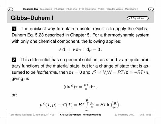
Ideal gas law Molecules Photons Phonons Free electrons Virial Van der Waals Murnaghan
7 Equations . . .Gibbs–Duhem I
1 The quickest way to obtain a useful result is to apply the Gibbs–Duhem Eq. 5.23 described in Chapter 5. For a thermodynamic systemwith only one chemical component, the folowing applies:
s dτ+ v dπ+ dµ = 0 .
2 This differential has no general solution, as s and v are quite arbi-trary functions of the material state, but for a change of state that is as-sumed to be isothermal, then dτ = 0 and v ıg = V/N = RT/p = −RT/π,giving us
(dµıg)T = RTπ dπ ,
or:
µıg(T , p) − µ(T) = RTp∫p
dππ = RT ln
(pp
).
Tore Haug-Warberg (ChemEng, NTNU) KP8108 Advanced Thermodynamics 23 February 2012 262 / 1598
Ideal gas law Molecules Photons Phonons Free electrons Virial Van der Waals Murnaghan
7 Equations . . .Gibbs–Duhem I (2)
Tore Haug-Warberg (ChemEng, NTNU) KP8108 Advanced Thermodynamics 23 February 2012 263 / 1598
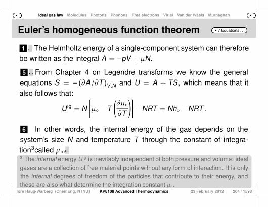
Ideal gas law Molecules Photons Phonons Free electrons Virial Van der Waals Murnaghan
7 Equations . . .Euler’s homogeneous function theorem
1 2 It is also important to remember that thermodynamic energy func-tions are first-order homogeneous functions to which Euler’s theoremapplies. The Helmholtz energy of a single-component system can therefore
be written as the integral A = −pV + µN.
5 3 Substituting in pıg and µıg from the above equations gives us:
A ıg = −NRT + Nµ(T) + NRT ln(
NRTpV
).
4 We have thus derived the Helmholtz energy from the ideal gas law,using the fact that Euler’s theorem applies to the extensive properties ofthe gas, and the Gibbs–Duhem equation, which is itself a direct resultof Euler’s theorem. From Chapter 4 on Legendre transforms we know the general
equations S = − (∂A/∂T)V ,N and U = A + TS, which means that italso follows that:
Uıg = N
[µ − T
(∂µ∂T
)]− NRT = Nh − NRT .
6 In other words, the internal energy of the gas depends on thesystem’s size N and temperature T through the constant of integra-tion3called µ.7 The latter constant must be determined experimentally in each in-
dividual case, or theoretically–experimentally if there are good simula-tion models for the chemical compound (based on spectrometric mea-surements).8 Our provisional conclusion is therefore that we can calculate the
Helmholtz energy of an ideal gas with only one chemical componentand its internal energy. From this the other energy functions can beobtained in a similar way using Legendre transforms, apart from onetemperature dependent constant.
3 The internal energy Uıg is inevitably independent of both pressure and volume: idealgases are a collection of free material points without any form of interaction. It is onlythe internal degrees of freedom of the particles that contribute to their energy, andthese are also what determine the integration constant µ.
Tore Haug-Warberg (ChemEng, NTNU) KP8108 Advanced Thermodynamics 23 February 2012 264 / 1598
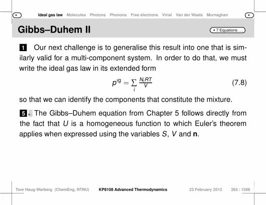
Ideal gas law Molecules Photons Phonons Free electrons Virial Van der Waals Murnaghan
7 Equations . . .Gibbs–Duhem II
1 Our next challenge is to generalise this result into one that is sim-ilarly valid for a multi-component system. In order to do that, we mustwrite the ideal gas law in its extended form
pıg =∑i
NiRTV (7.8)
so that we can identify the components that constitute the mixture.
5 2 This is a function of state in the form p(T ,V ,n), which gives us agood way to approach the question of Helmholtz energy A(T ,V ,n), butin order to determine A using the Euler method of integration as shownin Chapter 5, we also need to know the equation of state µıg
i (T ,V ,n).3 This function cannot be obtained experimentally in the same way
as pıg, and must therefore be derived theoretically.4 One way to do this is to apply the Gibbs–Duhem equation again:
S dτ+ V dπ+∑i
Ni dµi = 0 . The Gibbs–Duhem equation from Chapter 5 follows directly fromthe fact that U is a homogeneous function to which Euler’s theoremapplies when expressed using the variables S, V and n.
Tore Haug-Warberg (ChemEng, NTNU) KP8108 Advanced Thermodynamics 23 February 2012 265 / 1598
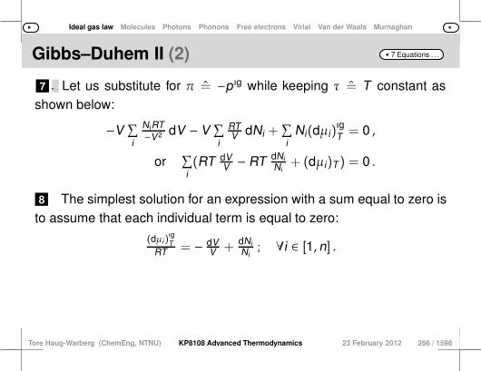
Ideal gas law Molecules Photons Phonons Free electrons Virial Van der Waals Murnaghan
7 Equations . . .Gibbs–Duhem II (2)
7 6 This means that there is an interdependence between the differ-entials of U which can be usefully exploited, and using the equation ofstate π = −pıg and the Gibbs–Duhem equation we will obtain a possi-ble solution for µi. Let us substitute for π = −pıg while keeping τ = T constant as
shown below:
−V∑i
NiRT−V2 dV − V
∑i
RTV dNi +
∑i
Ni(dµi)ıgT = 0 ,
or∑i(RT dV
V − RT dNiNi
+ (dµi)T ) = 0 .
8 The simplest solution for an expression with a sum equal to zero isto assume that each individual term is equal to zero:
(dµi)ıgT
RT = − dVV + dNi
Ni; ∀i ∈ [1, n] .
Tore Haug-Warberg (ChemEng, NTNU) KP8108 Advanced Thermodynamics 23 February 2012 266 / 1598

Ideal gas law Molecules Photons Phonons Free electrons Virial Van der Waals Murnaghan
7 Equations . . .Gibbs–Duhem II (3)
13 9 Thermodynamics is a phenomenological science, and we cannotbe sure that the above expression correctly describes the gas mixture,but at least it is a possible solution.10 However, the result agrees with experimental observations of dilutegases, which in the limit case p → 0 behave like a chaotic collection ofparticles without any interaction, and where the macroscopic propertiesassociated with each particle are independent of the other particles.11 Interestingly, deriving the chemical potiential of a component of anideal gas using statistical mechanics gives us exactly the same an-swera.12 This is a convincing demonstration of the great power of formalthermodynamic analysis.
a Statistical mechanical theory is based on a microscopic description of the propertiesof particles, and involves calculating their average values based on a relatively smallnumber of axioms. Whereas at the macroscopic level we have to accept that ourresult is merely a possible result, the theoretician can assert that it is a correct resultfor a gas consisting of hypothetical particles without any physical extension or mutualinteraction. In other words, a perfect gas. Integrating the differential gives us
1RT (µıg
i (T ,V ,n) − µi (T)) = − ln V
V+ ln Ni
Ni.
Note that the constant of integration µi , which will hereafter be calledthe standard state of component i, is a function of temperature.14 This means that for any given temperature T we must calculate or
estimate a new value for µi .15 If the function of state were available in the form p(S ,V ,n), then µiwould become a genuine constant of integration.16 In practice there are very few systems that can be described in thisway, but radiation from black bodies, as described in Paragraph 45, isone example.
Tore Haug-Warberg (ChemEng, NTNU) KP8108 Advanced Thermodynamics 23 February 2012 267 / 1598

Ideal gas law Molecules Photons Phonons Free electrons Virial Van der Waals Murnaghan
7 Equations . . .Standard potential
1 The normal convention is to assume a pure-component standardstate where V/Ni = RT/p and where p = 1 bar, or, in older referenceworks, where p = 1 atm.
3 2 The standard state µi should in that case be interpreted as rep-resenting µi (T , p), or more properly µıg
i (T , p,N1 = 0, . . . ,Ni = 1 mol,. . . ,Nn = 0). Bearing in mind this fundamental understanding of what µi means,
the chemical potential of the component can be expressed as
µıgi (T ,V ,n) = µi (T , p) + RT ln
(NiRTpV
). (7.9)
Here we should particularly note that (dµıgi )T ,V ,n = 0 must be true for all
values of p.
Tore Haug-Warberg (ChemEng, NTNU) KP8108 Advanced Thermodynamics 23 February 2012 268 / 1598

Ideal gas law Molecules Photons Phonons Free electrons Virial Van der Waals Murnaghan
7 Equations . . .Standard potential (2)
10 4 This is of course the case by definition, since T , V and n completelydetermine the thermodynamic state, but at the same time p acts as aparameter in the expression for µıg
i .5 It is therefore slightly unclear what happens if p changes.6 The passive role of the standard pressure becomes more obvious
if we partially differentiate µıgi with respect to p.
7 This gives us (∂µi /∂p)T − RT/p = 0, or put another way: if wechoose to change p then we must also correct µi to ensure that thetotal impact on µıg
i is zero.8 It is important for our own self-esteem to acknowledge that in or-
der to accurately determine the standard state one needs informationat a high level including precise calorimetric measurements, advancedspectroscopy and quantum physics, or a combination of these things,and that these activities lie outside our area of responsibility.9 We must therefore adapt our way of working to the available ther-
modynamic databases, and not vice-versa, which means that it is im-portant to use the data properly. Essentially, standard states are presented in three different ways in
the literature:
µi (T , p) = µi (T , p) (7.10)
µi (T , p) = ∆fhi (T) − Tsi (T , p) (7.11)
µi (T , p) = ∆fhi (T) + (hi (T) − hi (T)) − Tsi (T , p) . (7.12)
11 These equations follow from the definition G = U + pV − TS =
H − TS from Chapter 4 applied to the standard state as defined in theabove paragraph.
Tore Haug-Warberg (ChemEng, NTNU) KP8108 Advanced Thermodynamics 23 February 2012 269 / 1598
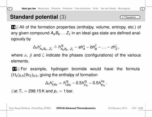
Ideal gas law Molecules Photons Phonons Free electrons Virial Van der Waals Murnaghan
7 Equations . . .Standard potential (3)
14 12 Moreover, it is an experimental fact that all molecules, with the ex-ception of monoatomic ones, have internal energy due to the bondingwithin the molecule.13 Normally this energy is reported as the enthalpy of formation∆fhi (T) of the compound. All of the formation properties (enthalpy, volume, entropy, etc.) of
any given compound AaBb . . .Zz in an ideal gas state are defined anal-ogously by
∆fhAaBb ...Zz
= hıgAaBb ...Zz
− ahαA − bhβB − . . . − zhζZ ,
where α, β and ζ indicate the phases (configurations) of the variouselements.
17 15 The phase can be liquid or solid, in which case the crystalline con-figuration is given, or a hypothetical ideal gas for gaseous elements.16 The chemical formula AaBb . . .Zz should here be seen as the ele-mental composition, i.e. not the atomic composition, of the molecule. For example, hydrogen bromide would have the formula
(H2)0.5(Br2)0.5, giving the enthalpy of formation
∆fhHBr = hıg
HBr− 0.5hıg
H2− 0.5h lıq
Br2.
18 The reason for this discrepancy, with respect to the establishedpractice for chemical equilibrium reactions, is that according to the IU-PAC convention the enthalpy of a chemical element is defined as zerofor the stable configuration of the elementa
a Such as H2(g), Ar(g), S(rhombıc), Br2(lıq), Al(s), etc. at T = 298.15 K and p = 1 bar.
Tore Haug-Warberg (ChemEng, NTNU) KP8108 Advanced Thermodynamics 23 February 2012 270 / 1598
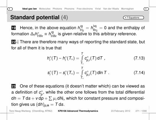
Ideal gas law Molecules Photons Phonons Free electrons Virial Van der Waals Murnaghan
7 Equations . . .Standard potential (4)
19 Hence, in the above equation hıgH2
= h lıqBr2
= 0 and the enthalpy offormation ∆fhHBr
≡ hıgHBr
is given relative to this arbitrary reference.
22 20 In particular, note that ∆fhBr2 , 0, as the enthalpy reference bydefinition relates to bromine in the liquid phase and not for bromine inthe (ideal) gas phase.21 This is the main principle that determines how the thermodynamicstandard state is reported, but there are, of course, exceptions to therule: at least one important database (JANAF) uses the more specificdefinition hi (T) = 0 for the elements at all temperatures T , while an-other database perhaps uses T = 0 K as its reference and yet anotherone may use gi (T, p) instead of si (T, p). There are therefore many ways of reporting the standard state, but
for all of them it is true that
hi (T) − hi (T) =T∫
T
cp,i(T)dT , (7.13)
si (T) − si (T) =T∫
T
cp,i(T)dln T . (7.14)
23 One of these equations (it doesn’t matter which) can be viewed asa definition of cp , while the other one follows from the total differentialdh = T ds + v dp +
∑µi dNi, which for constant pressure and composi-
tion gives us (dh)p,n = T ds.Tore Haug-Warberg (ChemEng, NTNU) KP8108 Advanced Thermodynamics 23 February 2012 271 / 1598

Ideal gas law Molecules Photons Phonons Free electrons Virial Van der Waals Murnaghan
7 Equations . . .The superposition principle
1 2 The sections 2.1–2.4 explain a little bit about the fundamental phys-ical principles that, in their different ways, contribute to cv,i . In practice, all thermodynamic reference works are based on a
large number of carefully recorded measurements supported by oneor more theoretical calculations, which together produce figures for∆fhi (T), si (T, p) and cp,i(T).
3 The enthalpy of formation is generally measured using calorimetry,whereas the heat capacity of an ideal gas component essentially ad-heres to the superposition principle 4
cp,i = c transv,i + crot
v,i + cvıbv,i + celec
v,i + R
and can be calculated from spectrometric measurements.4 The JANAF tablesa are a good example of how far this develop-ment has gone.5 For relatively small molecules (fewer than 8–10 atoms) it is nowpossible to estimate cp,i more precisely than using high-quality calori-metric measurements.a JANAF thermochemical tables. 3rd edition. Part I,II. J. Phys. Chem. Ref. Data, Suppl.,14(1), 1985.
4 The gas constant R in the above equation is a result of the defintiion of H = U + pV ,which for an ideal gas gives us Hıg = Uıg +(pV)ıg = Uıg +NRT . If we then differentiatewith respect to temperature we get cp,i = cv ,i + R.
Tore Haug-Warberg (ChemEng, NTNU) KP8108 Advanced Thermodynamics 23 February 2012 272 / 1598
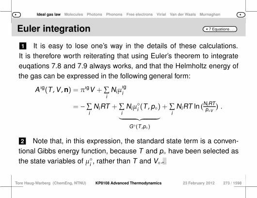
Ideal gas law Molecules Photons Phonons Free electrons Virial Van der Waals Murnaghan
7 Equations . . .Euler integration
1 It is easy to lose one’s way in the details of these calculations.It is therefore worth reiterating that using Euler’s theorem to integrateeuqations 7.8 and 7.9 always works, and that the Helmholtz energy ofthe gas can be expressed in the following general form:
A ıg(T ,V ,n) = πıgV +∑i
Niµıgi
= −∑i
NiRT +∑i
Niµi (T , p)
︸ ︷︷ ︸G(T ,p)
+∑i
NiRT ln(NiRT
pV
).
2 Note that, in this expression, the standard state term is a conven-tional Gibbs energy function, because T and p have been selected asthe state variables of µi , rather than T and V.3 In some strange manner, something has gone wrong here, but
what?4 It is clear that we no longer have a canonical description of
A (T ,V ,n), and that the unfortunate decision to combine T , V and n
from the original set of variables of p ıg, with p from the standard stateof µıg
i , is creating unintended confusion.
Tore Haug-Warberg (ChemEng, NTNU) KP8108 Advanced Thermodynamics 23 February 2012 273 / 1598

Ideal gas law Molecules Photons Phonons Free electrons Virial Van der Waals Murnaghan
7 Equations . . .Note 7.10
12 The consequences become even clearer if we take A ıg as our
starting point for differentiating Uıg = (∂(A ıg/T)/∂(1/T))V ,n or −S ıg =
(∂A ıg/∂T)V ,n.3 The partial derivative of A ıg is in both cases defined at constant
volume, but how is it possible to implement this for µi (T , p)?4 Let us use Uıg as an example.5 We start with
A ıg
T = −∑i
NiR +∑i
Niµi (T ,p)
T +∑i
NiR ln(NiRTpV )
6 followed by
d(A ıg
T )V ,n =∑i
Ni
(∂(µi /T)
∂(1/T)
)
p
d( 1T ) +
(∂(µi /T)
∂p
)
Tdp
−∑i
NiR[T d( 1
T ) +1p dp
].
7 Finally we use the Gibbs–Helmholtz equations from Paragraph 28on page 164 together with (∂(µi /T)/∂p)T = R/p from the equivalentdiscussion on page 256.8 The differential can now be expressed in the form
Uıg(T ,n) =(d(A ıg/T)
d(1/T)
)
V ,n=
∑i
Nihi (T) −∑i
NiRT = Hıg − pıgV ,
9 which shows that Uıg is only a function of T and n because p andV cancel out during the derivation.10 The total derivative now has one degree of freedom, and there-fore takes the same value as the partial derivative (∂(A ıg/T)/∂(1/T))
throughout the domain of definition.11 But why is it necessary to go via the total differential?12 Well, because otherwise we risk writing (∂(µi /T)/∂(1/T))V ,n = ui .13 Firstly µi is a function of V and not of V , and secondly V varieswith T when p has been chosen as the standard state.14 It is easy to make a mistake in those circumstances, and it is there-fore safest to go via the total differential.15 The derivation also illustrates how risky it is to introduce non-canonical variables for the thermodynamic potentials. In summary, the following equations apply to ideal gas mixtures:
A ıg(T ,V ,n) =∑i
Niµi (T , p) +
∑i
NiRT[ln
(NiRTpV
) − 1]
(7.15)
−S ıg(T ,V ,n) =∑i
Nisi (T , p) +∑i
NiR ln(NiRT
pV
)(7.16)
Uıg(T ,n) = Hıg(T ,n) − NRT (7.17)
Hıg(T ,n) =∑i
Nihi (T) . (7.18)
Tore Haug-Warberg (ChemEng, NTNU) KP8108 Advanced Thermodynamics 23 February 2012 274 / 1598
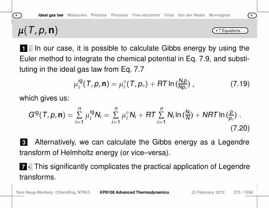
Ideal gas law Molecules Photons Phonons Free electrons Virial Van der Waals Murnaghan
7 Equations . . .µ(T , p,n)
1 2 Historicallly speaking, T , p,n has long been the favoured set ofvariables for modelling all chemical systems, probably because tem-perature and pressure are particularly easy to control in a laboratory. In our case, it is possible to calculate Gibbs energy by using the
Euler method to integrate the chemical potential in Eq. 7.9, and substi-tuting in the ideal gas law from Eq. 7.7
µıgi (T , p,n) = µi (T , p) + RT ln
(NipNp
), (7.19)
which gives us:
Gıg(T , p,n) =n∑
i=1µıg
i Ni =n∑
i=1µi Ni + RT
n∑i=1
Ni ln(Ni
N)+ NRT ln
( pp
).
(7.20)
3 Alternatively, we can calculate the Gibbs energy as a Legendretransform of Helmholtz energy (or vice–versa).
7 4 This is undoubtedly possible, but since Gıg and A ıg have differentcanonical variables, we also need to invert p(T ,V ,n) to V(T , p,n).5 If this is impossible, the result of the transformation will be an im-
plicit functiona.6 For most equations of state, with the exception of ideal gases, the
2nd virial equation and certain other models, an explicit transformationfrom T , p,n to T ,V ,n is impossible.
a The specification V(p) has 3 solutions in the steam/liquid phases, and is not a func-tion in the ordinary sense of the word. On the other hand, p(V) is an unambiguousspecification, which means that there is no problem with doing a Legendre transformof Helmholtz energy to Gibbs energy. This significantly complicates the practical application of Legendre
transforms.
Tore Haug-Warberg (ChemEng, NTNU) KP8108 Advanced Thermodynamics 23 February 2012 275 / 1598
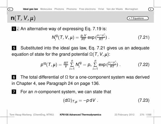
Ideal gas law Molecules Photons Phonons Free electrons Virial Van der Waals Murnaghan
7 Equations . . .n(T ,V ,µ)
1 2 The ideal gas law is a simple model, which allows us to choose anysystem variables that we like.3 For example, we can rewrite µ(T , p,n) or µ(T ,V ,n) as expressions
for n(T ,V ,µ).4 Very few models allow us to do this, and so we will make use of the
opportunity now that we have it. An alternative way of expressing Eq. 7.19 is:
Nıgi (T ,V ,µ) = pV
RT exp(µi−µi
RT). (7.21)
5 Substituted into the ideal gas law, Eq. 7.21 gives us an adequateequation of state for the grand potential Ω(T ,V ,µ):
pıg(T ,µ) = RTV
n∑i=1
Nıgi = p
n∑i=1
exp(µi−µi
RT). (7.22)
6 The total differential of Ω for a one-component system was derivedin Chapter 4, see Paragraph 24 on page 136.
7 For an n-component system, we can state that
(dΩ)T ,µ = −p dV . (7.23)
Tore Haug-Warberg (ChemEng, NTNU) KP8108 Advanced Thermodynamics 23 February 2012 276 / 1598

Ideal gas law Molecules Photons Phonons Free electrons Virial Van der Waals Murnaghan
7 Equations . . .n(T ,V ,µ) (2)
8 The differential (dΩ)T ,µ can be integrated directly, as long as thefunction of state p(T ,V ,µ) is expressed explicitly. Eq. 7.22 is explicit,and if we integrate using Euler’s method at a given T and µ we obtain
Ωıg(T ,V ,µ) = −pıgV = −pVn∑
i=1exp
(µi−µiRT
). (7.24)
9 It may at first sight appear that p is a free variable in the aboveequations, but if we change p, then µi (T , p) varies accordingly, alwayskeeping the value of Ωıg unchanged (show this).
11 10 Also note that pıg(T , µi) is a function of only two variables inEq. 7.22, whereas Ωıg(T ,V , µi) in Eq. 7.24 requires three variables. The intensive state is evidently given when n + 1 intensive vari-
ables have been determined, while the extensive state requires n + 2variables.
12 This is a general result, which is not limited to ideal gases5.13 From Paragraph 35 in Chapter 5 we know that the partial differen-tials of functions with only one extensive variable fulfil the requirementsfor homogeneitya:
∂T∂S
p,µ1,...,µn =
∂p∂V
T ,µ1,...,µn =
∂µ1
∂N1
T ,p,µ2,...,µn
= . . . =∂µn
∂Nn
T ,p,µ1,...,µn−1
= 0 .
14 The intensive variables are clearly independent of the size of thesystem, and the state is therefore given when n + 1 intensive variableshave been determined, cf. Paragraph 39 on page 214.15 However, in order to determine the size of the system, we alsoneed an extensive variable.16 In other words, a thermodynamic system requires n + 2 state vari-ables, in spite of the fact that the intensive state can be described withonly n + 1 variables.
a Zero is zero, most people probably think, but the partial differentials have differentunits in this case, and the similarity only applies to the measure (the absolute value) ofthese quantities.
5 In contrast to e.g. Uıg = U(T ,n), which only applies to ideal gases.Tore Haug-Warberg (ChemEng, NTNU) KP8108 Advanced Thermodynamics 23 February 2012 277 / 1598

Ideal gas law Molecules Photons Phonons Free electrons Virial Van der Waals Murnaghan
7 Equations . . .§ 040 § 39 § 41
Derive the partial derivatives of Ωıg(T ,V , µj) with respectto T , V and µi. Show that the results can be interpreted
as −S ıg, −pıg and −Nıgj , without discussing the properties
of the Legendre transform.
Tore Haug-Warberg (ChemEng, NTNU) KP8108 Advanced Thermodynamics 23 February 2012 278 / 1598
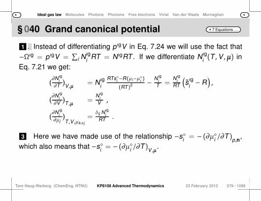
Ideal gas law Molecules Photons Phonons Free electrons Virial Van der Waals Murnaghan
7 Equations . . .§ 040 Grand canonical potential
1 2 It’s a good idea to start by establishing some shadow values beforestarting on the differentiation process itself. Instead of differentiating pıgV in Eq. 7.24 we will use the fact that
−Ωıg = pıgV =∑
i Nıgi RT = NıgRT . If we differentiate Nıg
i (T ,V ,µ) inEq. 7.21 we get:
(∂Nıgi
∂T)V ,µ = Nıg
iRTsi −R(µi−µi )
(RT)2 − Nıgi
T =Nıg
iRT
(sıg
i − R),
(∂Nıgi
∂V)T ,µ =
Nıgi
V ,
(∂Nıgi
∂µj
)T ,V ,µk,j
=δij Nıg
iRT .
3 Here we have made use of the relationship −si = − (∂µi /∂T)p,n,which also means that −si = − (∂µi /∂T)
V ,µ.
Tore Haug-Warberg (ChemEng, NTNU) KP8108 Advanced Thermodynamics 23 February 2012 279 / 1598
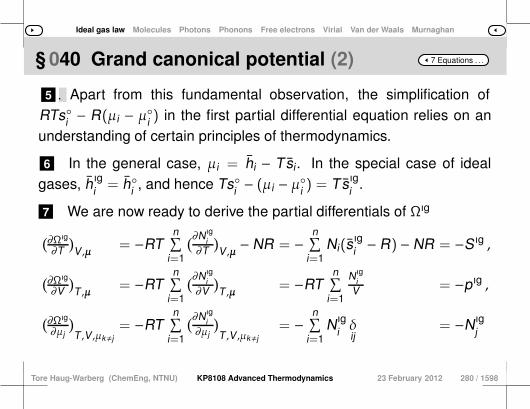
Ideal gas law Molecules Photons Phonons Free electrons Virial Van der Waals Murnaghan
7 Equations . . .§ 040 Grand canonical potential (2)
5 4 Think about this result for a moment. Apart from this fundamental observation, the simplification ofRTsi − R(µi − µi ) in the first partial differential equation relies on anunderstanding of certain principles of thermodynamics.
6 In the general case, µi = hi − Tsi. In the special case of idealgases, hıg
i = hi , and hence Tsi − (µi − µi ) = Tsıgi .
7 We are now ready to derive the partial differentials of Ωıg
(∂Ωıg
∂T)V ,µ = −RT
n∑i=1
(∂Nıgi
∂T)V ,µ − NR = −
n∑i=1
Ni(sıgi − R) − NR = −S ıg ,
(∂Ωıg
∂V)T ,µ = −RT
n∑i=1
(∂Nıgi
∂V)T ,µ = −RT
n∑i=1
Nıgi
V = −pıg ,
(∂Ωıg
∂µj
)T ,V ,µk,j
= −RTn∑
i=1
(∂Nıgi
∂µj
)T ,V ,µk,j
= −n∑
i=1Nıg
i δij= −Nıg
j
Tore Haug-Warberg (ChemEng, NTNU) KP8108 Advanced Thermodynamics 23 February 2012 280 / 1598
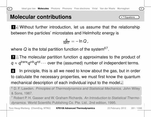
Ideal gas law Molecules Photons Phonons Free electrons Virial Van der Waals Murnaghan
7 Equations . . .Molecular contributions
1 2 The ideal gas law was established in several stages over the courseof the 17th-19th centuries, as an experimental law for the so-called per-manent gases (air, N2, H2, etc.).3 We now know that there is a direct link between the macroscopic
characteristics of the gas and the microscopic properties of the individ-ual molecules.4 The related discipline is called statistical mechanics or statistical
thermodynamics.5 It would be far too big a job to discuss this theory in detail, but
we will take the time to look at some of the details that underpin ourunderstanding of ideal gases. Without further introduction, let us assume that the relationship
between the particles’ microstates and Helmholtz energy is
ANRT = − ln Q ,
where Q is the total partition function of the system67.
7 6 For a system with n particles in defined locations, Q = qn, but ifthe particles are not in a fixed location (as in a gas), then Q = 1
n!qn. The molecular partition function q approximates to the product of
q ≈ qtransqvıbqrot · · · over the (assumed) number of independent terms.
8 In principle, this is all we need to know about the gas, but in orderto calculate the necessary properties, we must first know the quantummechanical description of each individual input to the model.9 We can only barely scratch the surface of quantum mechanics, and
the descriptions given in this section have therefore been kept as simpleas possible.10 However, before we start looking at microstates, we will first estab-lish the fundamental macroscopic thermodynamic equations that applyto ideal gases.
6 D. F. Lawden. Principles of Thermodynamics and Statistical Mechanics. John Wiley& Sons, 1987.7 Robert P. H. Gasser and W. Graham Richards. An Introduction to Statistical Thermo-dynamics. World Scientific Publishing Co. Pte. Ltd., 2nd edition, 1995.
Tore Haug-Warberg (ChemEng, NTNU) KP8108 Advanced Thermodynamics 23 February 2012 281 / 1598

Ideal gas law Molecules Photons Phonons Free electrons Virial Van der Waals Murnaghan
7 Equations . . .Free translation
1 A particle-in-a-box has three identical degrees of translational free-dom.
3 2 Even though the particle can in principle move freely within thecontrol volume, its kinetic energy is quantified (only standing waves arepermitted). In a cubic box, each direction will have its own quantum number jx ,
jy and jz , which is given the same unit of energy ε = h2/8ml2.
4 The associated partition function8 can be written
qtrans =∞∑
jx=1
∞∑jy=1
∞∑jz=1
exp(−(j2x+j2y+j2z )ε
kT).
5 For high quantum numbers j2 = j2x + j2y + j2z ≫ 0 is a virtuallycontinuous function over (an eighth of) the surface of a sphere with aradius of j.
Tore Haug-Warberg (ChemEng, NTNU) KP8108 Advanced Thermodynamics 23 February 2012 282 / 1598
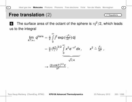
Ideal gas law Molecules Photons Phonons Free electrons Virial Van der Waals Murnaghan
7 Equations . . .Free translation (2)
6 The surface area of the octant of the sphere is πj2/2, which leadsus to the integral
limkT≫ε
qtrans = π2
∞∫
0
j2 exp(−j2ε
kT)dj
= π2(kTε
)3/2∞∫
0
x2e−x2dx
︸ ︷︷ ︸√π/4
, x2 =j2εkT ,
→ (2πmkT)3/2Vh3 .
Tore Haug-Warberg (ChemEng, NTNU) KP8108 Advanced Thermodynamics 23 February 2012 283 / 1598

Ideal gas law Molecules Photons Phonons Free electrons Virial Van der Waals Murnaghan
7 Equations . . .Free translation (3)
7 When going from summation to integration, it has been assumedthat kT ≫ εx . Combining this with j2 ≫ 0 gives us j2ε/kT < 1 overmuch of the area of integration, which ensures that the integral is agood approximation of the sum.
8 Per Chr. Hemmer. Statistisk mekanikk. Tapir Forlag, 1970. In Norwegian.
Tore Haug-Warberg (ChemEng, NTNU) KP8108 Advanced Thermodynamics 23 February 2012 284 / 1598
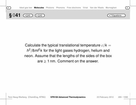
Ideal gas law Molecules Photons Phonons Free electrons Virial Van der Waals Murnaghan
7 Equations . . .§ 041 § 40 § 42
Calculate the typical translational temperature ε/k =
h2/8ml2k for the light gases hydrogen, helium andneon. Assume that the lengths of the sides of the box
are ≥ 1 nm. Comment on the answer.
Tore Haug-Warberg (ChemEng, NTNU) KP8108 Advanced Thermodynamics 23 February 2012 285 / 1598

Ideal gas law Molecules Photons Phonons Free electrons Virial Van der Waals Murnaghan
7 Equations . . .§ 041 Particle-in-a-box
1 The table below gives the values for ε/k and the standard boil-ingpoint of these three low-boiling-point compounds.
Mwg/mol
ε/kK
TbK
H2 2.0159 1.19 20.39He 4.0026 0.60 4.224Ne 20.179 0.12 27.09
2 The length of the sides of the box is l = 1 nm (which is right at thelimit of the range of validity of classical thermodynamics).
3 Except in the case of He, ε/k is reassuringly far below the boilingpoint of the compounds, and in practice all gases have a virtually con-tinuous spectrum of translational energies9.9 Note that ε ∝ l-2. If the length of the box is changed to e.g. 10 nm, then ε/k will bereduced by a factor of 100. This means that even He behaves in the classical mannerin a macroscopic control volume.Tore Haug-Warberg (ChemEng, NTNU) KP8108 Advanced Thermodynamics 23 February 2012 286 / 1598
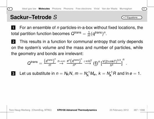
Ideal gas law Molecules Photons Phonons Free electrons Virial Van der Waals Murnaghan
7 Equations . . .Sackur–Tetrode S
1 For an ensemble of n particles-in-a-box without fixed locations, thetotal partition function becomes Q trans = 1
n!(qtrans)n.
2 This results in a function for communal entropy that only dependson the system’s volume and the mass and number of particles, whilethe geometry and bonds are irrelevant:
Q trans =(qtrans)
n
n!n→∞→ en(qtrans)
n
nnε≪kT−→ (e
n)n [V(2πmkT)3/2
h3
]n.
3 Let us substitute in n = NAN, m = N-1A Mw , k = N-1
A R and ln e = 1.
Tore Haug-Warberg (ChemEng, NTNU) KP8108 Advanced Thermodynamics 23 February 2012 287 / 1598
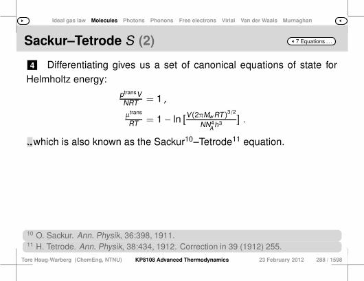
Ideal gas law Molecules Photons Phonons Free electrons Virial Van der Waals Murnaghan
7 Equations . . .Sackur–Tetrode S (2)
4 Differentiating gives us a set of canonical equations of state forHelmholtz energy:
ptransVNRT = 1 ,
µtrans
RT = 1 − ln[V(2πMw RT)3/2
NN4A h3
].
5 Two of thermodynamic properties that can be derived from this arectrans
v /R = 3/2 and standard entropy
strans(1 atm)R = −1.164855 . . .+ 5
2 ln T[K] +
32 ln Mw
[g/mol] , which is also known as the Sackur10–Tetrode11 equation.
10 O. Sackur. Ann. Physik, 36:398, 1911.11 H. Tetrode. Ann. Physik, 38:434, 1912. Correction in 39 (1912) 255.
Tore Haug-Warberg (ChemEng, NTNU) KP8108 Advanced Thermodynamics 23 February 2012 288 / 1598
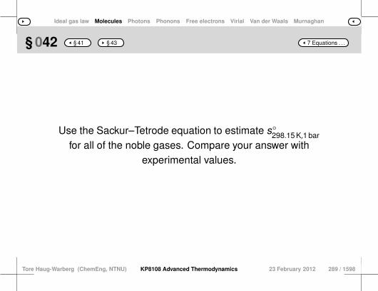
Ideal gas law Molecules Photons Phonons Free electrons Virial Van der Waals Murnaghan
7 Equations . . .§ 042 § 41 § 43
Use the Sackur–Tetrode equation to estimate s298.15 K,1 barfor all of the noble gases. Compare your answer with
experimental values.
Tore Haug-Warberg (ChemEng, NTNU) KP8108 Advanced Thermodynamics 23 February 2012 289 / 1598

Ideal gas law Molecules Photons Phonons Free electrons Virial Van der Waals Murnaghan
7 Equations . . .§ 042 Sackur–Tetrode
1 A convincing comparison of measured and calculated values isshown in Table 7.1.
2 These calculations are more precise than experimental results, butthe theory cannot be tested on multi-atomic molecules, because theinternal degrees of freedom of the molecules also contribute energy.3 This topic will be further discussed in the following sections on vi-
brational and rotational degrees of freedom.
Tore Haug-Warberg (ChemEng, NTNU) KP8108 Advanced Thermodynamics 23 February 2012 290 / 1598
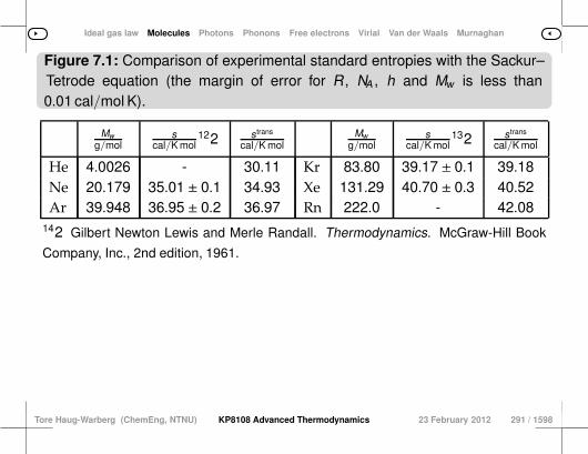
Ideal gas law Molecules Photons Phonons Free electrons Virial Van der Waals Murnaghan
Figure 7.1: Comparison of experimental standard entropies with the Sackur–Tetrode equation (the margin of error for R , NA , h and Mw is less than0.01 cal/mol K).
Mwg/mol
scal/K mol
122 strans
cal/K molMw
g/mols
cal/K mol132 strans
cal/K mol
He 4.0026 - 30.11 Kr 83.80 39.17 ± 0.1 39.18Ne 20.179 35.01 ± 0.1 34.93 Xe 131.29 40.70 ± 0.3 40.52Ar 39.948 36.95 ± 0.2 36.97 Rn 222.0 - 42.08
142 Gilbert Newton Lewis and Merle Randall. Thermodynamics. McGraw-Hill Book
Company, Inc., 2nd edition, 1961.
Tore Haug-Warberg (ChemEng, NTNU) KP8108 Advanced Thermodynamics 23 February 2012 291 / 1598
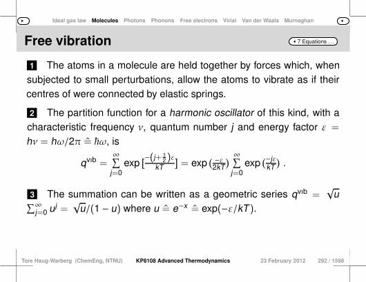
Ideal gas law Molecules Photons Phonons Free electrons Virial Van der Waals Murnaghan
7 Equations . . .Free vibration
1 The atoms in a molecule are held together by forces which, whensubjected to small perturbations, allow the atoms to vibrate as if theircentres of were connected by elastic springs.
2 The partition function for a harmonic oscillator of this kind, with acharacteristic frequency ν, quantum number j and energy factor ε =
hν = hω/2π = ~ω, is
qvıb =∞∑
j=0exp
[−(j+ 12)ε
kT]= exp
( −ε2kT
) ∞∑j=0
exp(−jε
kT).
3 The summation can be written as a geometric series qvıb =√
u∑∞j=0 uj =
√u/(1 − u) where u = e−x = exp(−ε/kT).
Tore Haug-Warberg (ChemEng, NTNU) KP8108 Advanced Thermodynamics 23 February 2012 292 / 1598
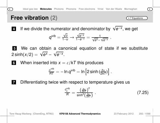
Ideal gas law Molecules Photons Phonons Free electrons Virial Van der Waals Murnaghan
7 Equations . . .Free vibration (2)
4 If we divide the numerator and denominator by√
e−x , we get
qvıb =√
u1−u →
√e−x
1−e−x = 1√ex−√
e−x.
5 We can obtain a canonical equation of state if we substitute2 sinh(x/2) =
√ex −
√e−x .
6 When inserted into x = ε/kT this produces
µvıb
RT = − ln qvıb = ln[2 sinh
( hν2kT
)].
7 Differentiating twice with respect to temperature gives us
cvıbv
R =( hν
2kT )2
sinh2( hν2kT )
. (7.25)
Tore Haug-Warberg (ChemEng, NTNU) KP8108 Advanced Thermodynamics 23 February 2012 293 / 1598
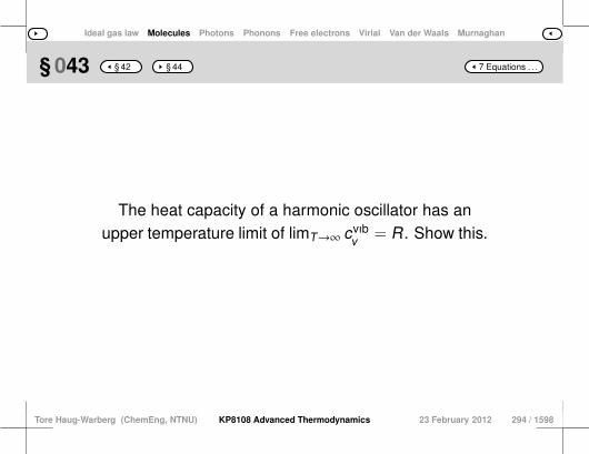
Ideal gas law Molecules Photons Phonons Free electrons Virial Van der Waals Murnaghan
7 Equations . . .§ 043 § 42 § 44
The heat capacity of a harmonic oscillator has anupper temperature limit of limT→∞ cvıb
v = R. Show this.
Tore Haug-Warberg (ChemEng, NTNU) KP8108 Advanced Thermodynamics 23 February 2012 294 / 1598
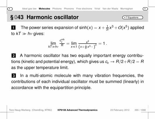
Ideal gas law Molecules Photons Phonons Free electrons Virial Van der Waals Murnaghan
7 Equations . . .§ 043 Harmonic oscillator
1 The power series expansion of sinh(x) = x + 13!x
3 +O(x5) appliedto kT ≫ hν gives:
limkT≫hν
cvıbv
R = limx≪1
x2
(x+ 13!x
3···)2 = 1 .
2 A harmonic oscillator has two equally important energy contribu-tions (kinetic and potential energy), which gives us cv → R/2+R/2 = Ras the upper temperature limit.
3 In a multi-atomic molecule with many vibration frequencies, thecontributions of each individual oscillator must be summed (linearly) inaccordance with the equipartition principle.
Tore Haug-Warberg (ChemEng, NTNU) KP8108 Advanced Thermodynamics 23 February 2012 295 / 1598
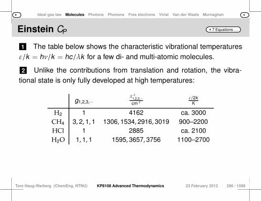
Ideal gas law Molecules Photons Phonons Free electrons Virial Van der Waals Murnaghan
7 Equations . . .Einstein CP
1 The table below shows the characteristic vibrational temperaturesε/k = hν/k = hc/λk for a few di- and multi-atomic molecules.
2 Unlike the contributions from translation and rotation, the vibra-tional state is only fully developed at high temperatures:
g1,2,3,···λ-11,2,3,···cm-1
ε/2kK
H2 1 4162 ca. 3000CH4 3, 2, 1, 1 1306, 1534, 2916, 3019 900–2200HCl 1 2885 ca. 2100H2O 1, 1, 1 1595, 3657, 3756 1100–2700
Tore Haug-Warberg (ChemEng, NTNU) KP8108 Advanced Thermodynamics 23 February 2012 296 / 1598
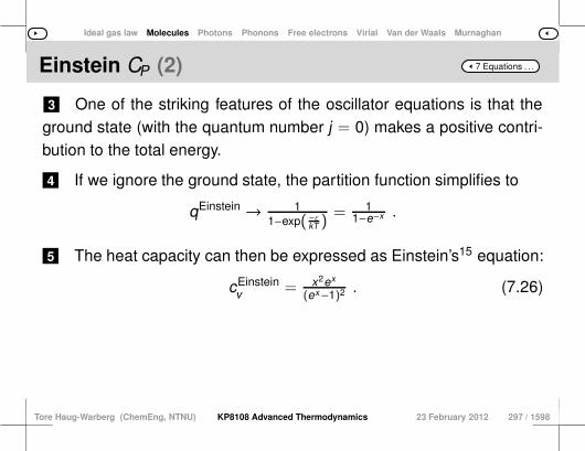
Ideal gas law Molecules Photons Phonons Free electrons Virial Van der Waals Murnaghan
7 Equations . . .Einstein CP (2)
3 One of the striking features of the oscillator equations is that theground state (with the quantum number j = 0) makes a positive contri-bution to the total energy.
4 If we ignore the ground state, the partition function simplifies to
qEinstein → 11−exp( −εkT )
= 11−e−x .
5 The heat capacity can then be expressed as Einstein’s15 equation:
cEinsteinv = x2ex
(ex−1)2 . (7.26)
Tore Haug-Warberg (ChemEng, NTNU) KP8108 Advanced Thermodynamics 23 February 2012 297 / 1598
Ideal gas law Molecules Photons Phonons Free electrons Virial Van der Waals Murnaghan
7 Equations . . .Einstein CP (3)
6 Our intuition tells us that the Eqs. 7.25 and 7.26 are equiva-lent, because the ground state only makes a constant (temperature-independent) energy contribution. The explanation for this is by nomeans obvious at first glance, but if we compare the equations, we cansee that it is the case (show this).
15 Albert Einstein, 1879–1955. German physicist.
Tore Haug-Warberg (ChemEng, NTNU) KP8108 Advanced Thermodynamics 23 February 2012 298 / 1598
Ideal gas law Molecules Photons Phonons Free electrons Virial Van der Waals Murnaghan
7 Equations . . .Free rotation
1 A rotating system with a fixed distribution of mass is called a rigidrotor. The moment of inertia of the rotor determines how much kineticenergy it stores at any given frequency.
2 In quantum mechanics, the moment of inertia of isolated atoms iszero, whereas diatomic (linear) molecules have degenerate moments ofinertia about two of their axes of rotation and a zero moment of inertiaabout the third axis.
3 In multi-atomic (non-linear) molecules, the moments of inertiaabout each axis of rotation are different, unless the symmetry of themolecule dictates otherwise.
Tore Haug-Warberg (ChemEng, NTNU) KP8108 Advanced Thermodynamics 23 February 2012 299 / 1598

Ideal gas law Molecules Photons Phonons Free electrons Virial Van der Waals Murnaghan
7 Equations . . .Free rotation (2)
4 The partition function for a linear molecule with a moment of inertiaI, quantum number j and energy factor ε = ~2/2I = h2/8π2I can beexpressed
qrot,2D = 1σ
∞∑j=0
(2j + 1)exp[−j(j+1)ε
kT],
where σ corrects for any rotational symmetry of the molecule (σH2O = 2,σNH3 = 3, σCH4 = 12).
5 There is no analytical limit to the above summation, but expandingthe power series16 gives us qrot = kT
ε (1 + ε3kT + 1
15(ε
kT )2 + 4
315(ε
kT )3 +
· · · ) provided that 0.3kT > ε.
Tore Haug-Warberg (ChemEng, NTNU) KP8108 Advanced Thermodynamics 23 February 2012 300 / 1598
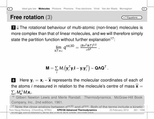
Ideal gas law Molecules Photons Phonons Free electrons Virial Van der Waals Murnaghan
7 Equations . . .Free rotation (3)
7 6 The upper temperature limit can be calculated using integration toobtain an approximation of the partition sum, as shown below:
limkT≫ε
qrot,2D = 1σ
∞∫
j=0
(2j + 1)exp[−j(j+1)ε
kT]dj
= − kTσε e−j(j+1) εkT
∣∣∣∞0→ 8π2IkT
σh2 . The rotational behaviour of multi-atomic (non-linear) molecules ismore complex than that of linear molecules, and we will therefore simplystate the partition function without further explanation17:
limkT≫ε
qrot,3D =(8π2IkT)3/2
σh3 .
M =∑i
Mi
(yT
i yiI − yiyTi
)∼ QΛQT .
8 Here yi = xi − x represents the molecular coordinates of each ofthe atoms i measured in relation to the molecule’s centre of mass x =∑
i M-1w Mixi.
16 Gilbert Newton Lewis and Merle Randall. Thermodynamics. McGraw-Hill BookCompany, Inc., 2nd edition, 1961.17 Note the close analogy between qrot,3D and qtrans. Both of the terms include a kineticenergy contribution, and so there are clear similarties.
Tore Haug-Warberg (ChemEng, NTNU) KP8108 Advanced Thermodynamics 23 February 2012 301 / 1598

Ideal gas law Molecules Photons Phonons Free electrons Virial Van der Waals Murnaghan
7 Equations . . .§ 044 § 43 § 45
Determine the moment of inertia of an H2O moleculeif the bond angle is 104.5 and the O–H distance is
0.958 Å.
Tore Haug-Warberg (ChemEng, NTNU) KP8108 Advanced Thermodynamics 23 February 2012 302 / 1598

Ideal gas law Molecules Photons Phonons Free electrons Virial Van der Waals Murnaghan
7 Equations . . .§ 044 Moment of inertia
1 Let us number the atoms H(1), H(2) and O(3).
2 Their respsective atomic weights are M1 = 1.00794 gmol-1, M2 =
1.00794 gmol-1 and M3 = 15.9994 gmol-1.
3 The molecule can be oriented in an infinite number of ways, andthe coordinates given below are simply based on an arbitrary choice(origin at O(3) and H(1) along the x axis):
x1
[Å]=
−.95800
, x2
[Å]=
0.958 · sin(14.5·2π360 ) = 0.240
0.958 · cos(14.5·2π360 ) = 0.927
0
, x3
[Å]=
000
.
Tore Haug-Warberg (ChemEng, NTNU) KP8108 Advanced Thermodynamics 23 February 2012 303 / 1598
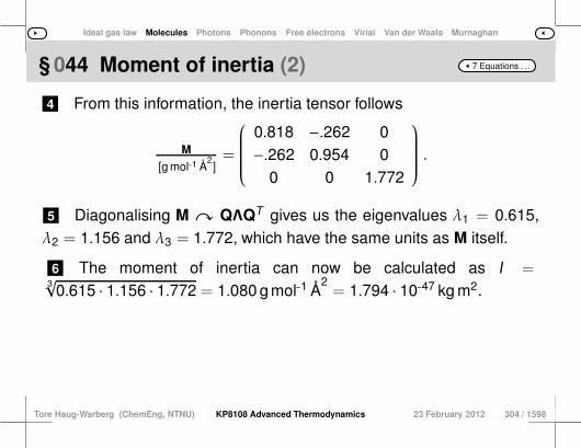
Ideal gas law Molecules Photons Phonons Free electrons Virial Van der Waals Murnaghan
7 Equations . . .§ 044 Moment of inertia (2)
4 From this information, the inertia tensor follows
M
[g mol-1 Å2]=
0.818 −.262 0−.262 0.954 0
0 0 1.772
.
5 Diagonalising M y QΛQT gives us the eigenvalues λ1 = 0.615,λ2 = 1.156 and λ3 = 1.772, which have the same units as M itself.
6 The moment of inertia can now be calculated as I =3√0.615 · 1.156 · 1.772 = 1.080 g mol-1 Å
2= 1.794 · 10-47 kg m2.
Tore Haug-Warberg (ChemEng, NTNU) KP8108 Advanced Thermodynamics 23 February 2012 304 / 1598

Ideal gas law Molecules Photons Phonons Free electrons Virial Van der Waals Murnaghan
7 Equations . . .Non-linear molecules
1 Finally, the canonical equation of state describing the rotation ofnon-linear molecules can be written
µrot,3D = −RT ln (8π2IRT)3/2
σN3A h3 ,
as long as we understand that I = 3√λ1λ2λ3 represents the molar mo-ment of inertia.
2 Most molecules, with the exception of hydrogen (isotopes), there-fore have a relatively high moment of inertia, which means that the up-per temperature limit is as low as T . 50 K:
Tore Haug-Warberg (ChemEng, NTNU) KP8108 Advanced Thermodynamics 23 February 2012 305 / 1598

Ideal gas law Molecules Photons Phonons Free electrons Virial Van der Waals Murnaghan
7 Equations . . .Non-linear molecules (2)
Ref.18 σ λi ·1047
kg m2I·1047
kg m2ε/kK
TbK
H2 2 0.460 0.460 0 0.460 87.6 20.39CH4 12 5.313 5.313 5.313 5.313 7.6 111.66HCl 1 2.641 2.641 0 2.641 15.3 188.15H2O 2 1.022 1.920 2.942 1.794 22.5 373.15
3 This gives us the classical heat capacity values of R and 3/2R forlinear and non-linear molecules respectively.
18 G. M. Barrow. Physical Chemistry. McGraw-Hill, 3rd edition, 1979.
Tore Haug-Warberg (ChemEng, NTNU) KP8108 Advanced Thermodynamics 23 February 2012 306 / 1598
Ideal gas law Molecules Photons Phonons Free electrons Virial Van der Waals Murnaghan
7 Equations . . .Internal degrees of freedom
1 Vibration and rotation are the “classical” contributions to the intra-molecular energy function.
2 For simple molecules, these contributions can be added together,provided that the amplitude of vibration is small and doesn’t disturb themolecule’s centre of mass (harmonic oscillator).
3 However, the general description of the molecule is far more com-plex, and must take into account anharmonic vibration or internal rota-tional and torsional fluctuations.
4 In hydrocarbons, e.g. CH3, groups will rotate freely around thebond axis, whereas double bonds such as CH2 = CH2 only allow tor-sional fluctuations.5 Internal rotation can also be partially prevented by sufficiently low
temperatures (staggered rotation).6 An important theoretical limit in this context is the equipartition prin-
ciple, which states that a fully developed energy degree of freedom con-tributes 1
2R to cv (vibration results in two degrees of freedom, consist-ing of potential and kinetic energy).
Tore Haug-Warberg (ChemEng, NTNU) KP8108 Advanced Thermodynamics 23 February 2012 307 / 1598
Ideal gas law Molecules Photons Phonons Free electrons Virial Van der Waals Murnaghan
7 Equations . . .Electron excitation
1 Electron excitation is a phenomenon that typically occurs at hightemperatures, and the outer electrons in a stable molecule will (gradu-ally) be excited at temperatures & 3000 K.
2 In radicals, excitation can occur at . 1000 K, because their elec-trons are more weakly bonded.
Tore Haug-Warberg (ChemEng, NTNU) KP8108 Advanced Thermodynamics 23 February 2012 308 / 1598
Ideal gas law Molecules Photons Phonons Free electrons Virial Van der Waals Murnaghan
7 Equations . . .Quantum spin
1 The spin of elementary particles can also contribute to the energystate of a molecule.
2 In the case of hydrogen, nuclear spin (cf. parahydrogen and ortho-hydrogen) plays a key role at temperatures . 400 K.
3 Similarly, electron spin is significant if the molecule has unpairedelectrons (cf. NO, O2 and NO2).
Tore Haug-Warberg (ChemEng, NTNU) KP8108 Advanced Thermodynamics 23 February 2012 309 / 1598
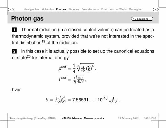
Ideal gas law Molecules Photons Phonons Free electrons Virial Van der Waals Murnaghan
7 Equations . . .Photon gas
1 Thermal radiation (in a closed control volume) can be treated as athermodynamic system, provided that we’re not interested in the spec-tral distribution19 of the radiation.
2 In this case it is actually possible to set up the canonical equationsof state20 for internal energy
prad =14
3√
34b
(SV)4,
T rad =3√
3S4bV ,
hvor
b = 8π5k4
15h3c3 = 7.56591 . . . · 10-16 Jm3 K4 .
Tore Haug-Warberg (ChemEng, NTNU) KP8108 Advanced Thermodynamics 23 February 2012 310 / 1598

Ideal gas law Molecules Photons Phonons Free electrons Virial Van der Waals Murnaghan
7 Equations . . .Photon gas (2)
6 3 Note that the number of photons present in the radiation space isnot included in the equations (determined by S and V ).4 In this respect eletromagnetic radiation deviates from the classical
notion that the particle number of a system can be treated as a freevariable because it is countable.5 An unexpected consequence of this is that the chemical potential
of the photon must be set at zero (this follows from a Lagrange optimi-sation of the equilibrium state). Using Euler’s method to do a simplified integration with respect to
only S and V gives us the internal energy of the radiation space:
Urad(S ,V) = T radS − pradV =34
3√
3S4
4bV .
7 By eliminating S we can obtain the Stefan21–Boltzmann22 law ofradiation Urad = bVT4. Alternatively, we can replace T with p, whichgives us Urad = 3pV .
19 An energy distribution function which has frequency as a free variable.20 Herbert Callen. Thermodynamics and an Introduction to Thermostatistics. Wiley,2nd edition, 1985.21 Jozef Stefan alias Joseph Stefan, 1835–1993. Slovenian physicist and poet.22 Ludwig Boltzmann, 1844–1906. Austrian physicist.
Tore Haug-Warberg (ChemEng, NTNU) KP8108 Advanced Thermodynamics 23 February 2012 311 / 1598
Ideal gas law Molecules Photons Phonons Free electrons Virial Van der Waals Murnaghan
7 Equations . . .§ 045 § 44 § 46
One of the most important fission reactions in a uraniumbomb can be written 1
0 n+23592 U→ 142
56 Ba+9136 Kr+1
0 n.The energy released is 3.5 · 10-11 J per fission event.Calculate T rad and prad if 1% of the atoms take part
in the fission reaction.
Tore Haug-Warberg (ChemEng, NTNU) KP8108 Advanced Thermodynamics 23 February 2012 312 / 1598

Ideal gas law Molecules Photons Phonons Free electrons Virial Van der Waals Murnaghan
7 Equations . . .§ 045 Atomic bomb
1 The density of the 235 uranium isotope is 19.1 g cm-3 and its molarmass is 235.04 gmol-1.
2 If 1% of the mass is involved in the reaction, the energy density willbe u = V -1U = 0.01 · 6.0221 · 1023 · 3.5 · 10-11 · 19.1 · 106/235.04 =
1.71 · 1016 J m-3.
3 From u = bT4 = 3p we can obtain T rad = 6.9 · 107 K and prad =
5.7 · 1010 bar.
4 These figures are representative for the uranium bomb Little Boy,which was dropped on Hiroshima on 6 August 1945.
Tore Haug-Warberg (ChemEng, NTNU) KP8108 Advanced Thermodynamics 23 February 2012 313 / 1598
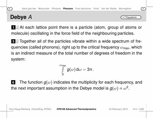
Ideal gas law Molecules Photons Phonons Free electrons Virial Van der Waals Murnaghan
7 Equations . . .Debye A
1 2 The Debyea
3 model of vibration is based on a periodic crystal lattice.
a Petrus Josephus Wilhelmus Debije, alias Peter Joseph William Debye, 1884–1966.Dutch–American physicist. At each lattice point there is a particle (atom, group of atoms or
molecule) oscillating in the force field of the neighbouring particles.
5 4 The partition function adheres to the Einstein model on page 284,but in such a way that the frequency can vary for each individual particle. Together all of the particles vibrate within a wide spectrum of fre-
quencies (called phonons), right up to the critical frequency ωmax, whichis an indirect measure of the total number of degrees of freedom in thesystem:
ωmax∫
0
g(ω)dω = 3n .
6 The function g(ω) indicates the multiplicity for each frequency, andthe next important assumption in the Debye model is g(ω) ∝ ω2.
Tore Haug-Warberg (ChemEng, NTNU) KP8108 Advanced Thermodynamics 23 February 2012 314 / 1598
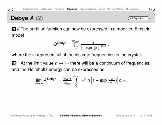
Ideal gas law Molecules Photons Phonons Free electrons Virial Van der Waals Murnaghan
7 Equations . . .Debye A (2)
9 7 This is not, of course, entirely accurate, but it is nevertheless amuch better assumption than saying that all of the particles vibrate withthe same frequency, as is assumed in the Einstein model.8 The explanation for thisa is complicated, so we will not dwell on it
here, but the result is incredibly simple
g(ω) = 9nω3max
ω2 .
a Herbert Callen. Thermodynamics and an Introduction to Thermostatistics. Wiley, 2ndedition, 1985. The partition function can now be expressed in a modified Einstein
model
QDebye =ωmax∏ω
1
[1−exp(−~ωkT )]g(ω) ,
where the ω represent all of the discrete frequencies in the crystal.
10 At the limit value n → ∞ there will be a continuum of frequencies,and the Helmholtz energy can be expressed as
limn→∞
ADebye = 9NRTω3
max
ωmax∫
0
ω2 ln[1 − exp
(−~ωkT
)]dω .
Tore Haug-Warberg (ChemEng, NTNU) KP8108 Advanced Thermodynamics 23 February 2012 315 / 1598
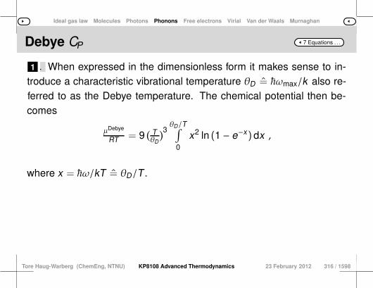
Ideal gas law Molecules Photons Phonons Free electrons Virial Van der Waals Murnaghan
7 Equations . . .Debye CP
1 2 The canonical equation of state can be obtained in the normal waythrough differentiation. When expressed in the dimensionless form it makes sense to in-
troduce a characteristic vibrational temperature θD = ~ωmax/k also re-ferred to as the Debye temperature. The chemical potential then be-comes
µDebye
RT = 9( TθD
)3 θD/T∫
0
x2 ln (1 − e−x)dx ,
where x = ~ω/kT = θD/T .
Tore Haug-Warberg (ChemEng, NTNU) KP8108 Advanced Thermodynamics 23 February 2012 316 / 1598

Ideal gas law Molecules Photons Phonons Free electrons Virial Van der Waals Murnaghan
7 Equations . . .Debye CP (2)
3 If we differentiate the partition function twice with respect to tem-perature, it gives us
cDebyev
R = 9( TθD
)3θD/T∫
0
x4ex
(ex−1)2 dx ,
but note that these expressions are two independent approximations ofthe partition function.
4 This introduces a thermodynamic inconsistency where cDebyev ,
−T ∂2µDebye/∂T∂T .
Tore Haug-Warberg (ChemEng, NTNU) KP8108 Advanced Thermodynamics 23 February 2012 317 / 1598

Ideal gas law Molecules Photons Phonons Free electrons Virial Van der Waals Murnaghan
7 Equations . . .Debye CP (3)
5 There is no analytical solution to the above integral, but at the uppertemperature limit θD/T → 0 and expanding the power series ex = 1 +
x + O(x2) gives us
limT→∞
cDebyev
R = 9( TθD
)3θD/T∫
0
x4(1+x+··· )(x+··· )2 dx ≃ 9
( TθD
)3θD/T∫
0
x2 dx = 3 .
6 This result shows that each atom (molecule) in the lattice oscillatesin 3 independent directions if the temperature is sufficiently high.
7 Many metals (Pb, Sn, Cd, Ag, . . . ) are essentially in this state atroom temperature. The limit value is also referred to as the Dulong–Petit23 law.
8 For the lower temperature limit, θD/T → ∞ and the integral is aconstant.
Tore Haug-Warberg (ChemEng, NTNU) KP8108 Advanced Thermodynamics 23 February 2012 318 / 1598
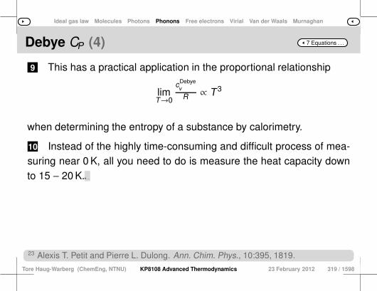
Ideal gas law Molecules Photons Phonons Free electrons Virial Van der Waals Murnaghan
7 Equations . . .Debye CP (4)
9 This has a practical application in the proportional relationship
limT→0
cDebyev
R ∝ T3
when determining the entropy of a substance by calorimetry.
10 Instead of the highly time-consuming and difficult process of mea-suring near 0 K, all you need to do is measure the heat capacity downto 15 − 20 K.11 Often this is sufficient to determine the factor of proportionality
in the above equation, allowing you to extrapolate the measurementsdown to 0 K.
23 Alexis T. Petit and Pierre L. Dulong. Ann. Chim. Phys., 10:395, 1819.
Tore Haug-Warberg (ChemEng, NTNU) KP8108 Advanced Thermodynamics 23 February 2012 319 / 1598
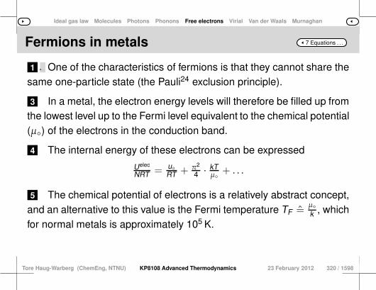
Ideal gas law Molecules Photons Phonons Free electrons Virial Van der Waals Murnaghan
7 Equations . . .Fermions in metals
1 2 The bonding electrons in a metal belong to a group of particlescalled fermions, named after the physicist Enrico Fermia.
a Enrico Fermi, 1901–1954. Italian–American physicist. One of the characteristics of fermions is that they cannot share thesame one-particle state (the Pauli24 exclusion principle).
3 In a metal, the electron energy levels will therefore be filled up fromthe lowest level up to the Fermi level equivalent to the chemical potential(µ) of the electrons in the conduction band.
4 The internal energy of these electrons can be expressed
Uelec
NRT = uRT + π2
4 · kTµ
+ . . .
5 The chemical potential of electrons is a relatively abstract concept,and an alternative to this value is the Fermi temperature TF =
µk , which
for normal metals is approximately 105 K.
Tore Haug-Warberg (ChemEng, NTNU) KP8108 Advanced Thermodynamics 23 February 2012 320 / 1598

Ideal gas law Molecules Photons Phonons Free electrons Virial Van der Waals Murnaghan
7 Equations . . .Fermions in metals (2)
6 Differentiating Uelec gives us the lower temperature limit for theelectronic contribution to the heat capacity of metals:
limT→0
celecv
R = π2T2TF∝ T .
7 This is in contrast to crystalline phases with covalent bonds wherelimT→0(cv) ∝ T3 due to the phonon contribution.
8 The practical implication of this is that the heat capacity of met-als is dominated by the fermion contribution at sufficiently low tempera-tures (T . 5 K).
24 Wolfgang Ernst Pauli, 1900–1958. Austrian physicist.
Tore Haug-Warberg (ChemEng, NTNU) KP8108 Advanced Thermodynamics 23 February 2012 321 / 1598

Ideal gas law Molecules Photons Phonons Free electrons Virial Van der Waals Murnaghan
7 Equations . . .Second virial coefficient
1 The virial equation relates to ideal gases. 2 There is an equivalent power series expansion for osmotic pressurein dilute solutions, but it is harder to derive. Expand the power se-
ries p/RT in molar density ρ = N/V :
pvırVNRT =
∞∑k=1
Bk (T)(NV)k−1
= 1 + B2(T) NV + · · · (7.27)
3 This is the normal way to express the virial development of gases,but it is also possible to invert the series from p(ρ) to ρ(p) as shownbelow.
4 Here the series has been truncated after the second term, whichmeans that the index 2 can be left off the symbol B:
pV2.vır
NRT = 1 + BNV + · · · ≃ 1 +
BpRT + · · ·
Tore Haug-Warberg (ChemEng, NTNU) KP8108 Advanced Thermodynamics 23 February 2012 322 / 1598
Ideal gas law Molecules Photons Phonons Free electrons Virial Van der Waals Murnaghan
7 Equations . . .Second virial coefficient (2)
5 Multiplying both sides by NRT/p gives the volume-explicit formV2.vır = NRT/p + BN, which reveals that B is a correction factor forthe molar volume of the gas.
6 Experimentally B = limp→0(V −RT/p) is used, but this limit tells usnothing about how B varies with temperature.
7 In practice B < 0 for T < TB ≈ 6Tc, where TB is known as theBoyle25 temperature.
Tore Haug-Warberg (ChemEng, NTNU) KP8108 Advanced Thermodynamics 23 February 2012 323 / 1598
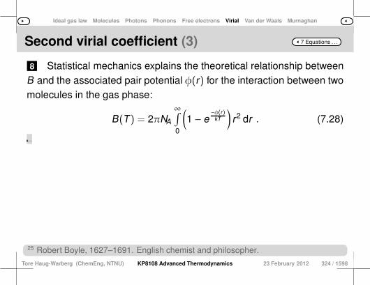
Ideal gas law Molecules Photons Phonons Free electrons Virial Van der Waals Murnaghan
7 Equations . . .Second virial coefficient (3)
8 Statistical mechanics explains the theoretical relationship betweenB and the associated pair potential φ(r) for the interaction between twomolecules in the gas phase:
B(T) = 2πNA
∞∫
0
(1 − e
−φ(r)kT
)r2 dr . (7.28)
9 This equation holds very well for non-polar molecules with vir-tually perfect spherical symmetry, but for rod-shaped molecules andmolecules with permanent dipole moments integration must be donewith respect to the (two) inter-molecular angles of orientation as well asthe inter-molecular distance.10 This results in an integral that looks like the one in 7.28, but whereφ(r) represents the mean pair potential of the molecules.
25 Robert Boyle, 1627–1691. English chemist and philosopher.
Tore Haug-Warberg (ChemEng, NTNU) KP8108 Advanced Thermodynamics 23 February 2012 324 / 1598

Ideal gas law Molecules Photons Phonons Free electrons Virial Van der Waals Murnaghan
7 Equations . . .Hard spheres
1
σ r
φLet us assume that φ = 0 for r > σ and φ = ∞for r ≤ σ.
2 That means viewing the molecules as hardspheres, with no pairwise interaction.
3 Substituting this into the integral for B givesus
Bhs = NA
σ∫
0
r2 dr = 2πNAσ3
3
4 The hard sphere potential produces a reasonable approximationof a real system at high temperatures, but it doesn’t explain why B istemperature-dependent.
Tore Haug-Warberg (ChemEng, NTNU) KP8108 Advanced Thermodynamics 23 February 2012 325 / 1598

Ideal gas law Molecules Photons Phonons Free electrons Virial Van der Waals Murnaghan
7 Equations . . .Potential well
1
−ε σ r
φLet us assume that φ = 0 for r > ασ, φ = −ε forσ < r ≤ ασ and φ = ∞ for r ≤ σ.
2 That means viewing the molecules as hardspheres with pairwise interaction within the po-tential well.
3 Substituting this simple potential into the integral for B (whereα > 1), demonstrates that B(T) is a strongly temperature-dependentfunction with the hard-sphere potential as its upper temperature limit:
Bsw = Bhs + 2πNA
ασ∫σ
(1 − e
εkT
)r2 dr
= Bhs[1 + (α3 − 1)(1 − e
εkT )
].
Tore Haug-Warberg (ChemEng, NTNU) KP8108 Advanced Thermodynamics 23 February 2012 326 / 1598
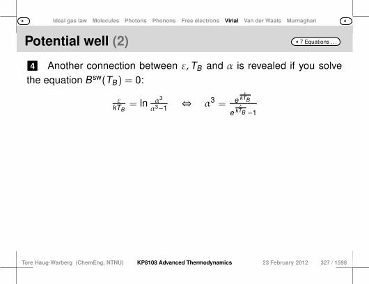
Ideal gas law Molecules Photons Phonons Free electrons Virial Van der Waals Murnaghan
7 Equations . . .Potential well (2)
4 Another connection between ε,TB and α is revealed if you solvethe equation Bsw(TB) = 0:
εkTB
= ln α3
α3−1 ⇔ α3 = eε
kTB
eε
kTB −1
Tore Haug-Warberg (ChemEng, NTNU) KP8108 Advanced Thermodynamics 23 February 2012 327 / 1598
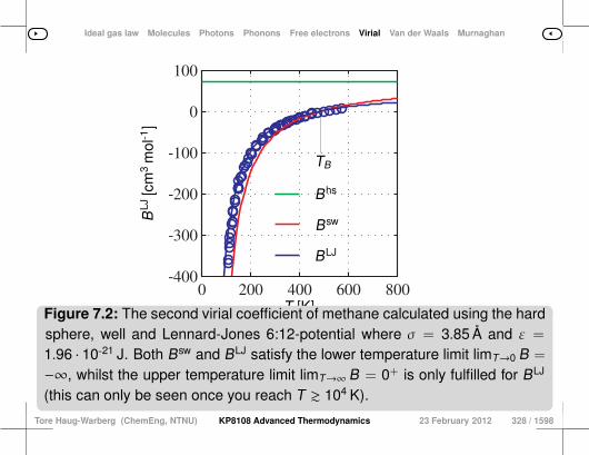
Ideal gas law Molecules Photons Phonons Free electrons Virial Van der Waals Murnaghan
0 200 400 600 800−400
−300
−200
−100
0
100
BLJ[c
m3
mol
-1]
T [K]
TB
Bhs
Bsw
BLJ
Figure 7.2: The second virial coefficient of methane calculated using the hardsphere, well and Lennard-Jones 6:12-potential where σ = 3.85 Å and ε =
1.96 · 10-21 J. Both Bsw and BLJ satisfy the lower temperature limit limT→0 B =
−∞, whilst the upper temperature limit limT→∞ B = 0+ is only fulfilled for BLJ
(this can only be seen once you reach T & 104 K).
Tore Haug-Warberg (ChemEng, NTNU) KP8108 Advanced Thermodynamics 23 February 2012 328 / 1598
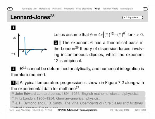
Ideal gas law Molecules Photons Phonons Free electrons Virial Van der Waals Murnaghan
7 Equations . . .Lennard-Jones28
1
−ε σ r
φLet us assume that φ = 4ε
[(σr )
12−(σr )6]
for r > 0.
3 2 This version is often referred to as the 6:12 potential. The exponent 6 has a theoretical basis inthe London26 theory of dispersion forces involv-ing instantaneous dipoles, whilst the exponent12 is empirical.
4 BLJ cannot be determined analytically, and numerical integration istherefore required.
7 5 This is simple in theory, but not quite so straightforward in practice.6 In order to prevent numerical problems, the lower limit is estimated
using a hard-sphere contribution and the upper limit using a power se-ries expansion, see the Matlab programme 30:1.5. A typical temperature progression is shown in Figure 7.2 along with
the experimental data for methane27.25 John Edward Lennard-Jones, 1894–1954. English mathematician and physicist.26 Fritz London, 1900–1954. German–american physicist.27 J. H. Dymond and E. B. Smith. The Virial Coefficients of Pure Gases and Mixtures.Oxford University Press, 1980.
Tore Haug-Warberg (ChemEng, NTNU) KP8108 Advanced Thermodynamics 23 February 2012 329 / 1598
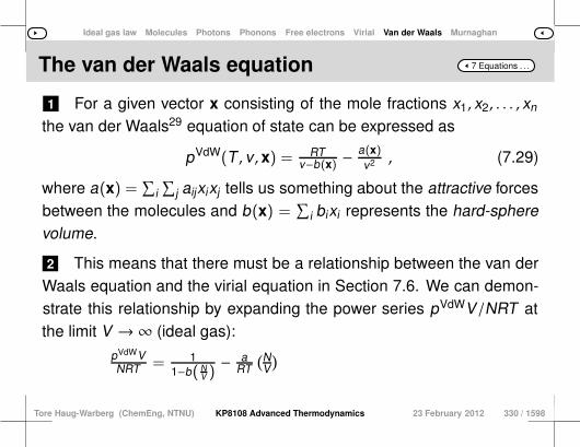
Ideal gas law Molecules Photons Phonons Free electrons Virial Van der Waals Murnaghan
7 Equations . . .The van der Waals equation
1 For a given vector x consisting of the mole fractions x1, x2, . . . , xn
the van der Waals29 equation of state can be expressed as
pVdW(T , v, x) = RTv−b(x) −
a(x)v2 , (7.29)
where a(x) =∑
i∑
j aijxixj tells us something about the attractive forcesbetween the molecules and b(x) =
∑i bixi represents the hard-sphere
volume.
2 This means that there must be a relationship between the van derWaals equation and the virial equation in Section 7.6. We can demon-strate this relationship by expanding the power series pVdWV/NRT atthe limit V →∞ (ideal gas):
pVdWVNRT = 1
1−b(NV )− a
RT(NV)
Tore Haug-Warberg (ChemEng, NTNU) KP8108 Advanced Thermodynamics 23 February 2012 330 / 1598
Ideal gas law Molecules Photons Phonons Free electrons Virial Van der Waals Murnaghan
7 Equations . . .The van der Waals equation (2)
= 1 + b(NV)+ b2 (N
V)2
+ · · ·+ bn (NV)n − a
RT(NV).
3 If we compare the coefficients in this series with the ones inEq. 7.27, we find that Bvdw
2 = b − a/RT , Bvdw3 = b2, Bvdw
4 = b3 etc.
6 4 Only Bvdw2 bears any resemblance to real systems; the other virial
coefficients are completely unrelated to reality.5 In spite of the massive simplification, the van der Waals equation
of state is often used as a starting point for more complicated equationsof state, see Chapter 13. It is beyond the scope of this chapter to discuss all of the impli-
cations of the van der Waals equation here, but we will at the veryleast note one important property: the parameters aii and bi can beobtained by measuring the critical point of each individual compoundexperimentally.7 This does not mean that the equation is valid under near-critical
conditions (it isn’t), but these parametric values produce universal be-haviour which is very valuable.
29 Johannes Diderik van der Waals, 1837–1923. Dutch physicist.
Tore Haug-Warberg (ChemEng, NTNU) KP8108 Advanced Thermodynamics 23 February 2012 331 / 1598
Ideal gas law Molecules Photons Phonons Free electrons Virial Van der Waals Murnaghan
7 Equations . . .§ 046 § 45 § 47
Show that the parameters b = RTc/8pc, vc = 3b anda = 27(RTc)
2/64pc meet the criteria for a mechanical–critical point defined by (∂p/∂v)T ,x = 0, (∂2p/∂v∂v)T ,x =
0 and p(Tc, vc) = pc.
Tore Haug-Warberg (ChemEng, NTNU) KP8108 Advanced Thermodynamics 23 February 2012 332 / 1598
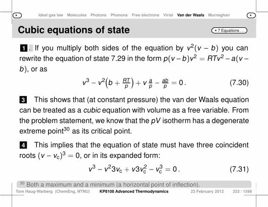
Ideal gas law Molecules Photons Phonons Free electrons Virial Van der Waals Murnaghan
7 Equations . . .Cubic equations of state
1 2 The values given can obviously be verified by direct substitution,but we will choose a different approach. If you multiply both sides of the equation by v2(v − b) you can
rewrite the equation of state 7.29 in the form p(v −b)v2 = RTv2−a(v −b), or as
v3 − v2(b + RT
p
)+ v a
p − abp = 0 . (7.30)
3 This shows that (at constant pressure) the van der Waals equationcan be treated as a cubic equation with volume as a free variable. Fromthe problem statement, we know that the pV isotherm has a degenerateextreme point30 as its critical point.
4 This implies that the equation of state must have three coincidentroots (v − vc)
3 = 0, or in its expanded form:
v3 − v23vc + v3v2c − v3
c = 0 . (7.31)
30 Both a maximum and a minimum (a horizontal point of inflection).Tore Haug-Warberg (ChemEng, NTNU) KP8108 Advanced Thermodynamics 23 February 2012 333 / 1598

Ideal gas law Molecules Photons Phonons Free electrons Virial Van der Waals Murnaghan
7 Equations . . .§ 046 Critical points
1 The two Eqs. 7.30 and 7.31 have the same algebraic structure,which allows us to compare the coefficients term by term.
2 This gives rise to the following set of equations:
3vc = b + RTcpc
,
3v2c = a
pc,
v3c = ab
pc,
which must be solved with respect to a, b and vc.
Tore Haug-Warberg (ChemEng, NTNU) KP8108 Advanced Thermodynamics 23 February 2012 334 / 1598

Ideal gas law Molecules Photons Phonons Free electrons Virial Van der Waals Murnaghan
7 Equations . . .§ 046 Critical points (2)
5 3 Alternatively we could have solved the equations with respect toe.g. a, b and R, but traditionally vc is favoured because it is subject to arelatively large degree of experimental uncertainty.4 However, this means that the van der Waals equation of state has
too few degrees of freedom to accurately reproduce all measurementsof pc,Tc and vc. The solution to the above set of equations can be expressed
38 =
vcpcRTc
, (7.32)
b = 13 vc , (7.33)
a = 3pcv2c , (7.34)
which can in turn be rewritten in the form used in the problem statement.
6 We should note that the critical compressibility factor zVdWc =
pcvc/RTc = 38 behaves as a universal constant because vc is a de-
pendent variable in the solution.
7 Experimentally this is no more than a rough approximation as0.25 < zc < 0.35 for most molecular compounds.
Tore Haug-Warberg (ChemEng, NTNU) KP8108 Advanced Thermodynamics 23 February 2012 335 / 1598
Ideal gas law Molecules Photons Phonons Free electrons Virial Van der Waals Murnaghan
7 Equations . . .§ 047 § 46 § 48
Pressure is an intensive property (homogeneous functionof degree zero), which implies that p(T , v, x) = p(T ,V ,n).
Rewrite the van der Waals Eq. 7.29 in this form.
Tore Haug-Warberg (ChemEng, NTNU) KP8108 Advanced Thermodynamics 23 February 2012 336 / 1598
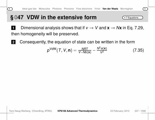
Ideal gas law Molecules Photons Phonons Free electrons Virial Van der Waals Murnaghan
7 Equations . . .§ 047 VDW in the extensive form
1 Dimensional analysis shows that if v → V and x→ Nx in Eq. 7.29,then homogeneity will be preserved.
2 Consequently, the equation of state can be written in the form
pVdW(T ,V ,n) = NRTV−Nb(x) −
N2a(x)V2 (7.35)
Tore Haug-Warberg (ChemEng, NTNU) KP8108 Advanced Thermodynamics 23 February 2012 337 / 1598

Ideal gas law Molecules Photons Phonons Free electrons Virial Van der Waals Murnaghan
7 Equations . . .§ 048 § 47 § 49
Show that, in its reduced form, the van der Waalsequation can be written as pr = 8Tr/ (3vr − 1)− 3/v2
r .Draw the function for Tr ∈ 0.75, 1, 1.5. Identify all ofthe asymptotes to the graph. Specify the physical
range of the function.
Tore Haug-Warberg (ChemEng, NTNU) KP8108 Advanced Thermodynamics 23 February 2012 338 / 1598
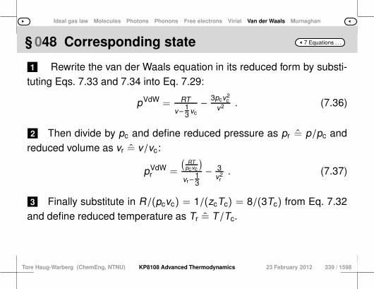
Ideal gas law Molecules Photons Phonons Free electrons Virial Van der Waals Murnaghan
7 Equations . . .§ 048 Corresponding state
1 Rewrite the van der Waals equation in its reduced form by substi-tuting Eqs. 7.33 and 7.34 into Eq. 7.29:
pVdW = RT
v−13 vc
− 3pcv2c
v2 . (7.36)
2 Then divide by pc and define reduced pressure as pr = p/pc andreduced volume as vr = v/vc:
pVdWr =
(RT
pcvc
)
vr−13
− 3v2
r. (7.37)
3 Finally substitute in R/(pcvc) = 1/(zcTc) = 8/(3Tc) from Eq. 7.32and define reduced temperature as Tr = T/Tc.
Tore Haug-Warberg (ChemEng, NTNU) KP8108 Advanced Thermodynamics 23 February 2012 339 / 1598
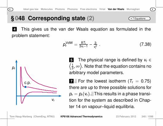
Ideal gas law Molecules Photons Phonons Free electrons Virial Van der Waals Murnaghan
7 Equations . . .§ 048 Corresponding state (2)
4 This gives us the van der Waals equation as formulated in theproblem statement:
pVdWr = 8Tr
3vr−1 − 3v2
r. (7.38)
vr
pr
bc.p.
5 The physical range is defined by vr ∈⟨13 ,∞
⟩. Note that the equation contains no
arbitrary model parameters.
7 6 We call this a universal equation, and here we will take the oppor-tunity to mention the principle of corresponding states, which states thatrelated substances behave virtually alike at reduced states. For the lowest isotherm (Tr = 0.75)
there are up to three possible solutions forpr = pr(vr). 8 The fluid is thermodynamically unstable in the range where
(∂pr/∂vr) > 0. This results in a phase transi-tion for the system as described in Chap-ter 14 on vapour–liquid equilibria.
Tore Haug-Warberg (ChemEng, NTNU) KP8108 Advanced Thermodynamics 23 February 2012 340 / 1598

Ideal gas law Molecules Photons Phonons Free electrons Virial Van der Waals Murnaghan
7 Equations . . .Condensed phases
1 According to Murnaghan31’s equation, isobaric expansivity α andisothermal compressibility β are two independent state functions of tem-perature and pressure respectively. 2 The equation is most useful for pure solids and stoichiometric com-
pounds.3 To derive the chemical potential, we start with the total differential
of molar volume, for our current purposes expressed as (dln v)murN =
α(T )dT − β(p)dp, also see Section 8.6 on page 385.
4 Two commonly used functions for α and β are:
α(T) = a1 + a2T +a3T2 ,
β(p) = b11+b2p .
5 Let us start by integrating α(T) at a given reference pressure pbetween the reference temperature T and an arbitrary system temper-ature T . This gives us: ln[v(T , p)/v(T, p)] = a1(T − T) + 1
2a2(T2 −T2 ) − a3(T -1 − T -1
) = (T − T)[a1 +12a2(T + T) + a3(TT)-1].
Tore Haug-Warberg (ChemEng, NTNU) KP8108 Advanced Thermodynamics 23 February 2012 341 / 1598

Ideal gas law Molecules Photons Phonons Free electrons Virial Van der Waals Murnaghan
7 Equations . . .Condensed phases (2)
6 Next we integrate β(p) at constant T between the reference pres-sure p and an arbitrary system pressure p. This gives us: ln[v(T , p)/v(T , p)] = −b -1
2 b1 ln[(1 + b2p)/(1 + b2p)].
7 We can now integrate (dµ)T ,N = v dp between the two states T , pand T , p. This produces µmur(T , p) = µ(T , p) +
∫ pp
v(T , p)dp whichwith a little bit of effort can be rewritten as
µmur(T , p) = µ(T , p) + v(T , p)p∫p
( 1+b2p1+b2p
)−b1/b2dp
= µ(T , p) + v(T , p)1+b2pb2−b1
[( 1+b2p1+b2p
)1−b1/b2 − 1]
= µ(T , p) +b1
b2−b1
vβ
[ββ
vv− 1
],
where β = β(p) and v = v(T , p).8 It is now easy to produce a complete equation of state µmur(T ,p),provided that we have an expression for the compound’s standardchemical potential µ(T ,p).9 For solid phases at high pressures and polymorphous compounds,
it is normal to express the standard molar Gibbs energy as a (kind of)power series of temperature:
µRT = . . .+ a
T2 + bT + c + d ln
(TT
)+ eT + fT2 + . . .
10 A trivial integration of µmur using the Euler method gives us theGibbs energy function
Gmur(T ,p,N) = Nµmur(T ,p) .
31 F. D. Murnaghan. Proc. Natl. Acad. Sci. U. S. A., 30:244–247, 1944.
Tore Haug-Warberg (ChemEng, NTNU) KP8108 Advanced Thermodynamics 23 February 2012 342 / 1598
Ideal gas law Molecules Photons Phonons Free electrons Virial Van der Waals Murnaghan
7 Equations . . .§ 049 § 48 § 50
Murnaghan’s equation is derived by integrating theexpansivity with respect to T at a given p, and thenintegrating the compressibility with respect to p atconstant T , but this provides no guarantee that our
starting point was thermodynamically consistent. Usedifferentiation to show that α = f(T) and β = g(p)
genuinely represent a consistent basis for a model.
Tore Haug-Warberg (ChemEng, NTNU) KP8108 Advanced Thermodynamics 23 February 2012 343 / 1598

Ideal gas law Molecules Photons Phonons Free electrons Virial Van der Waals Murnaghan
7 Equations . . .§ 049 The Murnaghan model
1 2 It is easy to make apparently independent assumptions withoutchecking whether they are mutually coherent. For the model to be consistent, the third-order Maxwell equation
∂2v∂T∂p = ∂2v
∂p∂T
must hold. Substituting in (∂v/∂T)p = vf(T) and (∂v/∂p)T = −vg(p)gives us
− (∂v∂T
)p g(p) ?
=(∂v∂p
)T
f(T) ,
where f(T) and g(p) are functions of different state variables.
4 3 This avoids circular references. If we rewrite the last equation slightly we get
vf(T)g(p) ?= vg(p)f(T) .
Here the right-hand side is identical to the left-hand side, so the test hasbeen satisfied.
Tore Haug-Warberg (ChemEng, NTNU) KP8108 Advanced Thermodynamics 23 February 2012 344 / 1598
Ideal gas law Molecules Photons Phonons Free electrons Virial Van der Waals Murnaghan
7 Equations . . .§ 050 § 49 § 51
Assume that thermal expansivity is constant, i.e. thata2 = 0 K-2 and a3 = 0 K. Find an expression for
(∂cp/∂p)T ,N that is true for this simplified Murnaghanmodel. What is the sign of the derivative?
Tore Haug-Warberg (ChemEng, NTNU) KP8108 Advanced Thermodynamics 23 February 2012 345 / 1598
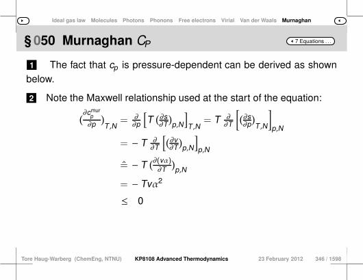
Ideal gas law Molecules Photons Phonons Free electrons Virial Van der Waals Murnaghan
7 Equations . . .§ 050 Murnaghan CP
1 The fact that cp is pressure-dependent can be derived as shownbelow.
2 Note the Maxwell relationship used at the start of the equation:
(∂cmurp
∂p
)T ,N
= ∂∂p
[T
(∂s∂T
)p,N
]T ,N
= T ∂∂T
[(∂s∂p
)T ,N
]
p,N
= − T ∂∂T
[(∂v∂T
)p,N
]p,N
= − T(∂(vα)∂T
)p,N
= − Tvα2
≤ 0
Tore Haug-Warberg (ChemEng, NTNU) KP8108 Advanced Thermodynamics 23 February 2012 346 / 1598
Ideal gas law Molecules Photons Phonons Free electrons Virial Van der Waals Murnaghan
7 Equations . . .§ 051 § 50 § 52
For a one-component system to be thermodynamicallystable, it must satisfy the conditions β > 0 and cp > 0.Are these conditions (always) met for Murnaghan’s
equation?
Tore Haug-Warberg (ChemEng, NTNU) KP8108 Advanced Thermodynamics 23 February 2012 347 / 1598
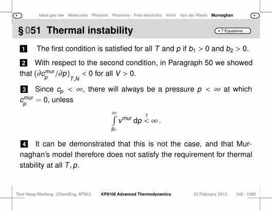
Ideal gas law Molecules Photons Phonons Free electrons Virial Van der Waals Murnaghan
7 Equations . . .§ 051 Thermal instability
1 The first condition is satisfied for all T and p if b1 > 0 and b2 > 0.
2 With respect to the second condition, in Paragraph 50 we showedthat (∂cmur
p /∂p)T ,N
< 0 for all V > 0.
3 Since cp < ∞, there will always be a pressure p < ∞ at whichcmur
p = 0, unless
∞∫p
vmur dp?< ∞ .
4 It can be demonstrated that this is not the case, and that Mur-naghan’s model therefore does not satisfy the requirement for thermalstability at all T , p.
Tore Haug-Warberg (ChemEng, NTNU) KP8108 Advanced Thermodynamics 23 February 2012 348 / 1598
Gr,p(T ,p,n) Ar,p(T ,p,n) Ar,v(T ,V ,n)
Part 13
Departure Functions
see also Part-Contents
Tore Haug-Warberg (ChemEng, NTNU) KP8108 Advanced Thermodynamics 23 February 2012 677 / 1598
Gr,p(T ,p,n) Ar,p(T ,p,n) Ar,v(T ,V ,n)
Contents
1 Gr,p(T , p,n)
2 A r,p(T , p,n)
1 Physical derivation2 Rational derivation3 Connection with Gibbs energy
3 A r,v(T ,V ,n)
Tore Haug-Warberg (ChemEng, NTNU) KP8108 Advanced Thermodynamics 23 February 2012 678 / 1598
Gr,p(T ,p,n) Ar,p(T ,p,n) Ar,v(T ,V ,n)
13 Departure . . .Multicomponent thermodynamics
1 From a thermodynamic point of view, it makes little differencewhether a system is composed of one, two or many components, pro-vided that their relative proportions are constant in time and space.
4 2 Such systems will only have three degrees of freedoma
3 and will have relatively simple descriptions, as discussed in Chap-ter 8 on page 342.
a Chemical reactions change the mole numbers of the compounds in a system withoutaffecting the components that only vary with mass, i.e. the atoms or atom groups thatare reaction invariant. The internal degrees of freedom are hidden from the outsideworld, so the composition of the system is perceived to be constant, although the sizeof the system may well vary with e.g. temperature and pressure. The situation becomes much more complicated, however, if the
components that vary with mass are included in the system description.
5 The number of degrees of freedom increases, and the thermody-namic functions describe abstract hyperplanes in more than three spa-tial dimensions.
6 This makes it difficult to visualise the mathematical description, andas we do not want to restrict the theory to any specific chemical system,we shall hereafter use generic indices i ∈ [1, n] instead of componentnames.
Tore Haug-Warberg (ChemEng, NTNU) KP8108 Advanced Thermodynamics 23 February 2012 679 / 1598
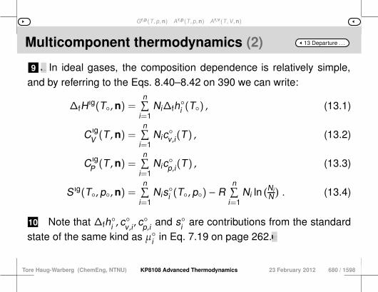
Gr,p(T ,p,n) Ar,p(T ,p,n) Ar,v(T ,V ,n)
13 Departure . . .Multicomponent thermodynamics (2)
9 7 The thermodynamics of multi-component mixtures therefore has amore formal structure than that of its single-component counterpart.8 The virial equation will be used repeatedly as an example in this
chapter, but let us start by looking at how we can extend the resultsfrom Chapter 8 on page 342 to systems with variable compositions. In ideal gases, the composition dependence is relatively simple,
and by referring to the Eqs. 8.40–8.42 on 390 we can write:
∆fHıg(T,n) =
n∑i=1
Ni∆fhi (T) , (13.1)
C ıgV (T ,n) =
n∑i=1
Nicv,i(T) , (13.2)
C ıgP (T ,n) =
n∑i=1
Nicp,i(T) , (13.3)
S ıg(T, p,n) =n∑
i=1Nisi (T, p) − R
n∑i=1
Ni ln(Ni
N). (13.4)
10 Note that ∆fhi , cv,i , c
p,i and si are contributions from the standard
state of the same kind as µi in Eq. 7.19 on page 262.11 For systems with constant composition, U, H and S are the keyfunctions, but in mixtures the chemical potential becomes increasinglyimportant.12 However, this quantity cannot be obtained by differentiatingU or H with respect to their canonical variables because µi =
(∂U/∂Ni)S ,V ,Nj,i = (∂H/∂Ni)S,p,Nj,i
13 requires S to be a free variable, which is only possible in very spe-cial cases.14 The solution to the problem is to take either the Gibbsa or theHelmholtzb energy as our starting point, as µi = (∂G/∂Ni)T ,p,Nj,i =
(∂A/∂Ni)T ,V ,Nj,i
15 can then be determined through explicit differentiationc.16 Whether we use G or A depends on the equation of state beingused (more on this later).
a Josiah Willard Gibbs, 1839–1903. American physicist.b Hermann Ludwig Ferdinand von Helmholtz, 1821–1894. German physician andphysicist.c The great majority of thermodynamic models, including both equations of state andactivity coefficient models, are explicit in T but not in S .
Tore Haug-Warberg (ChemEng, NTNU) KP8108 Advanced Thermodynamics 23 February 2012 680 / 1598
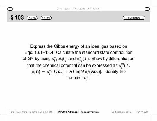
Gr,p(T ,p,n) Ar,p(T ,p,n) Ar,v(T ,V ,n)
13 Departure . . .§ 103 § 102 § 104
Express the Gibbs energy of an ideal gas based onEqs. 13.1–13.4. Calculate the standard state contribution
of Gıg by using si , ∆fhi and cp,i(T). Show by differentiation
that the chemical potential can be expressed as µıgi (T ,
p,n) = µi (T , p) + RT ln[Nip/(Np)]. Identify thefunction µi .
Tore Haug-Warberg (ChemEng, NTNU) KP8108 Advanced Thermodynamics 23 February 2012 681 / 1598
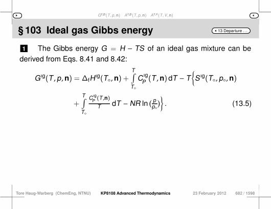
Gr,p(T ,p,n) Ar,p(T ,p,n) Ar,v(T ,V ,n)
13 Departure . . .§ 103 Ideal gas Gibbs energy
1 The Gibbs energy G = H − TS of an ideal gas mixture can bederived from Eqs. 8.41 and 8.42:
Gıg(T , p,n) = ∆fHıg(T,n) +
T∫
T
C ıgP (T ,n)dT − T
S ıg(T, p,n)
+T∫
T
C ıgP (T ,n)
T dT − NR ln( pp
). (13.5)
Tore Haug-Warberg (ChemEng, NTNU) KP8108 Advanced Thermodynamics 23 February 2012 682 / 1598
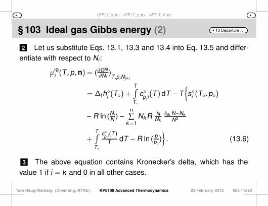
Gr,p(T ,p,n) Ar,p(T ,p,n) Ar,v(T ,V ,n)
13 Departure . . .§ 103 Ideal gas Gibbs energy (2)
2 Let us substitute Eqs. 13.1, 13.3 and 13.4 into Eq. 13.5 and differ-entiate with respect to Ni:
µıgi (T , p,n) =
(∂Gıg
∂Ni
)T ,p,Nj,i
= ∆fhi (T) +
T∫
T
cp,i(T)dT − Tsi (T, p)
− R ln(Ni
N) −
n∑k=1
Nk R NNk
δik N−NkN2
+T∫
T
cp,i(T)
T dT − R ln( pp
). (13.6)
3 The above equation contains Kronecker’s delta, which has thevalue 1 if i = k and 0 in all other cases.
Tore Haug-Warberg (ChemEng, NTNU) KP8108 Advanced Thermodynamics 23 February 2012 683 / 1598
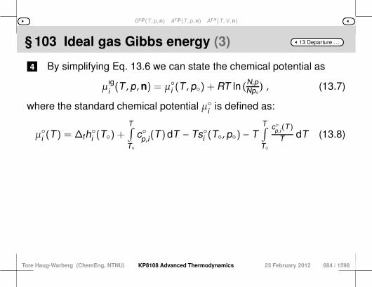
Gr,p(T ,p,n) Ar,p(T ,p,n) Ar,v(T ,V ,n)
13 Departure . . .§ 103 Ideal gas Gibbs energy (3)
4 By simplifying Eq. 13.6 we can state the chemical potential as
µıgi (T , p,n) = µi (T , p) + RT ln
(NipNp
), (13.7)
where the standard chemical potential µi is defined as:
µi (T) = ∆fhi (T) +
T∫
T
cp,i(T)dT − Tsi (T, p) − TT∫
T
cp,i(T)
T dT (13.8)
Tore Haug-Warberg (ChemEng, NTNU) KP8108 Advanced Thermodynamics 23 February 2012 684 / 1598

Gr,p(T ,p,n) Ar,p(T ,p,n) Ar,v(T ,V ,n)
13 Departure . . .§ 104 § 103 § 105
Use a specific example to show that Uıg − TS ıg +
pV ıg =∑n
i=1 µıgi Ni.
Tore Haug-Warberg (ChemEng, NTNU) KP8108 Advanced Thermodynamics 23 February 2012 685 / 1598
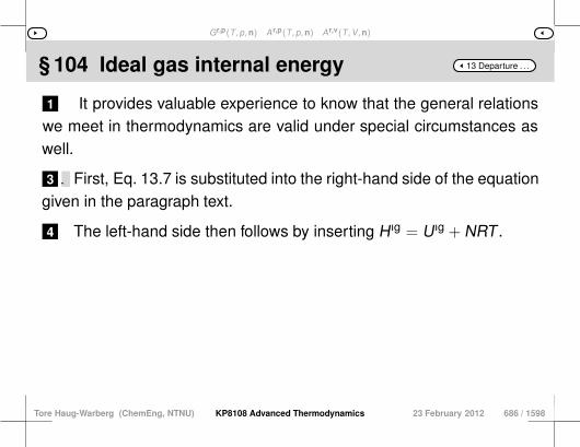
Gr,p(T ,p,n) Ar,p(T ,p,n) Ar,v(T ,V ,n)
13 Departure . . .§ 104 Ideal gas internal energy
1 It provides valuable experience to know that the general relationswe meet in thermodynamics are valid under special circumstances aswell.
3 2 This paragraph underpins such an experience. First, Eq. 13.7 is substituted into the right-hand side of the equationgiven in the paragraph text.
4 The left-hand side then follows by inserting Hıg = Uıg + NRT .
Tore Haug-Warberg (ChemEng, NTNU) KP8108 Advanced Thermodynamics 23 February 2012 686 / 1598
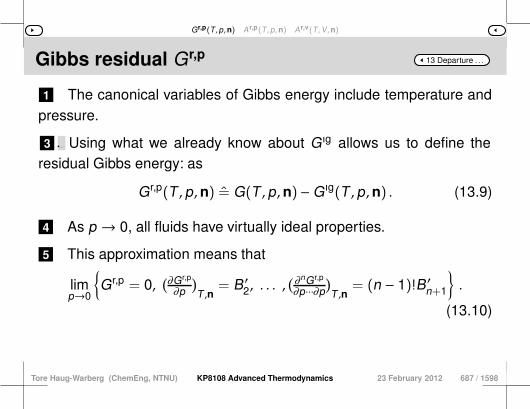
Gr,p(T ,p,n) Ar,p(T ,p,n) Ar,v(T ,V ,n)
13 Departure . . .Gibbs residual Gr,p
1 The canonical variables of Gibbs energy include temperature andpressure.
3 2 This makes it possible to compare the chemical potentials of thecomponents of real fluids with those of the same components in theideal gas state, at the same temperature and pressure. Using what we already know about Gıg allows us to define the
residual Gibbs energy: as
Gr,p(T , p,n) = G(T , p,n)−Gıg(T , p,n) . (13.9)
4 As p → 0, all fluids have virtually ideal properties.
5 This approximation means that
limp→0
Gr,p = 0,
(∂Gr,p
∂p
)T ,n
= B ′2, . . . ,(∂nGr,p
∂p···∂p
)T ,n
= (n − 1)!B ′n+1
.
(13.10)
Tore Haug-Warberg (ChemEng, NTNU) KP8108 Advanced Thermodynamics 23 February 2012 687 / 1598

Gr,p(T ,p,n) Ar,p(T ,p,n) Ar,v(T ,V ,n)
13 Departure . . .Gibbs residual Gr,p (2)
6 This is consistent with the virial theorem in Chapter 7 on page 242,and with the Legendre transform in Chapter 4, from which it follows that(∂G/∂p)T ,n is the system volume regardless of whether the fluid is idealor real.
7 By taking the limits from Eq. 13.10 it is possible to rewrite Eq. 13.9as1:
Gr,p(T , p,n) =p∫
0
(V − V ıg)dπ =p∫
0
(V(π) − NRT
π
)dπ . (13.11)
1 Note that π is used as the integration variable in order to avoid confusion with p,which appears in the upper limit of the integral.
Tore Haug-Warberg (ChemEng, NTNU) KP8108 Advanced Thermodynamics 23 February 2012 688 / 1598

Gr,p(T ,p,n) Ar,p(T ,p,n) Ar,v(T ,V ,n)
13 Departure . . .Residual chemical potential
1 An equivalent expression for the chemical potential µi =
(∂G/∂Ni)T ,p,Nj,iis true for all conceivable Gibbs energy functions, in-
cluding Gr,p.
2 This allows us to define the residual chemical potential as µr,pi =
µi − µıgi , or
µr,pi (T , p,n) =
(∂Gr,p
∂Ni
)T ,p,Nj,i
=p∫
0
[(∂V∂Ni
)T ,π,Nj,i
− RTπ
]dπ =
p∫
0
(vi − RT
π
)dπ , (13.12)
where vi = (∂V/∂Ni)T ,π,Nj,iis the partial molar volume of the component
i.3 To obtain Eq. 13.12 from Eq. 13.11, Gr,p must be differentiated atconstant pressurea.
a Note that to calculate the derivative of Gr,p at a given pressure p we must know thederivative of V − V ıg for all pressures π ∈ [0,p] in the integration domain. This goesagainst usual practice when performing partial differentiation, but Gr,p is a functionalthat is defined for all pressures p > 0, and not merely for one arbitrarily chosen systempressure p. The integrand, on the other hand, only depends on the local pressure π, soit will not change in any way if p changes in the upper limit of the integral. The integral inquestion is thus uniquely defined in terms of the area under a specific curve, integratedfrom the lower limit p = 0 up to the system pressure p. Admittedly the curve dependson the specified isotherm T and specified composition n, but it does not depend on thesystem pressure p. Consequently, the curve must be defined by differentiating V −V ıg
at every value of π such that we can choose to stop the integration at any value ofp > 0.
Tore Haug-Warberg (ChemEng, NTNU) KP8108 Advanced Thermodynamics 23 February 2012 689 / 1598

Gr,p(T ,p,n) Ar,p(T ,p,n) Ar,v(T ,V ,n)
13 Departure . . .The derivative of an integral
1 Since the system pressure is only present in the limit of the integral,we need only worry about the derivative of the kernel, but there thepressure does vary (locally) throughout the integration!
2 This is an unusual situation, and it is important to realise that thecorresponding differential of V(π) is defined locally as
(dV)T ,π,Nj,i =(∂V∂Ni
)T ,π,Nj,i
dNi
for all pressures π ∈ [0, p].3 What is unusual in this respect is that there are two different phys-ical interpretions of pressure — one being the system pressure in theupper limit of the integral and the other being the integration variable π.
Tore Haug-Warberg (ChemEng, NTNU) KP8108 Advanced Thermodynamics 23 February 2012 690 / 1598
Gr,p(T ,p,n) Ar,p(T ,p,n) Ar,v(T ,V ,n)
13 Departure . . .The derivative of an integral (2)
4 However, there is a given local pressure π at each stage of the in-tegration, so the only remaining degree of freedom comes from varia-tion in the composition of component i.
5 Hence, the chemical potential must be integrated over the volumederivative as shown in Eq. 13.12.
6 For historical reasons it is customary to rewrite the residual poten-tial as
RT lnϕi = µr,pi (T , p,n) , (13.13)
where ϕi(T , p,n) is the fugacity coefficient of component i.7 This is a measure of the difference between the thermodynamicstate of a component in a real fluid and of the same component in idealgas under the system conditions T ,p,n.8 The fugacity coefficient has traditionally been given a great deal of
attention in the American literature, but really it is a vestige of the past.9 For gases at low pressures and phase equilibrium calculations us-
ing the K -value method it has certain benefits, but in general it causesmore problems than it solves — it neither increases our basic under-standing nor improves the numerical performance of thermodynamicalgorithms.
Tore Haug-Warberg (ChemEng, NTNU) KP8108 Advanced Thermodynamics 23 February 2012 691 / 1598
Gr,p(T ,p,n) Ar,p(T ,p,n) Ar,v(T ,V ,n)
13 Departure . . .§ 105 § 104 § 106
Show that µi = µıgi + µr,p
i = µi + RT ln[Niϕip/(Np)].Verify that the lower limit limp→0 ϕi = 1. What is ϕi for
a component in the ideal gas state?
Tore Haug-Warberg (ChemEng, NTNU) KP8108 Advanced Thermodynamics 23 February 2012 692 / 1598
Gr,p(T ,p,n) Ar,p(T ,p,n) Ar,v(T ,V ,n)
13 Departure . . .§ 105 The fugacity coefficient
1 The chemical potential can be derived by combining Eqs. 13.7 and13.12.
2 The latter equation gives us limp→0 µr,pi = 0 and hence limp→0 ϕi =
1.
3 For an ideal gas v ıgi = RT/π, which means that µr,p,ıg
i = 0 regard-less of the pressure.
4 Hence ϕıgi = 1.
Tore Haug-Warberg (ChemEng, NTNU) KP8108 Advanced Thermodynamics 23 February 2012 693 / 1598
Gr,p(T ,p,n) Ar,p(T ,p,n) Ar,v(T ,V ,n)
13 Departure . . .§ 106 § 105 § 107
Derive Gr,p for the 2nd virial equation if pV2.vır = NRT +Bp.Differentiate to find RT lnϕ2.vır
k . Use the quadraticmixing rule for B = N
∑i
∑j
xixjBi,j where Bi,j = Bj,i.
Tore Haug-Warberg (ChemEng, NTNU) KP8108 Advanced Thermodynamics 23 February 2012 694 / 1598
Gr,p(T ,p,n) Ar,p(T ,p,n) Ar,v(T ,V ,n)
13 Departure . . .§ 106 Virial Gibbs energy I
1 The residual Gibbs energy can be determined by directly substi-tuting the 2nd virial equation into Eq. 13.11:
Gr,p,2.vır =p∫
0
(NRTπ + B − NRT
π
)dπ = Bp . (13.14)
2 In order to find RT lnϕk we must differentiate Gr,p, and hence B,with respect to Nk , but differentiating with respect to (mole) fractionshas an unfortunate tendency to cause what is known as “code bloat” incomputing.
Tore Haug-Warberg (ChemEng, NTNU) KP8108 Advanced Thermodynamics 23 February 2012 695 / 1598
Gr,p(T ,p,n) Ar,p(T ,p,n) Ar,v(T ,V ,n)
13 Departure . . .§ 106 Virial Gibbs energy I (2)
3 We can considerably reduce the amount of writing that we needto do by using NB =
∑i∑
j NiNjBi,j, which, even though it is an implicitexpression, is much better suited for differentiation:
(∂NB∂Nk
)T ,Nl,k
=∑i
∑j
(∂NiNj
∂Nk
)Nl,k
Bij .
4 Differentiate both sides and substitute in Kronecker’s delta, whereδii = 1 if i = j and δij = 0 if i , j:
B + N( ∂B∂Nk
)T ,Nl,k
=∑i
∑j
(δik
Nj + Ni δjk
)Bij =
∑j
NjBkj +∑i
NiBik .
5 We can simplify the right-hand side considerably by substitutingBkj = Bjk and simultaneously changing one of the summation indicesfrom j to i.
Tore Haug-Warberg (ChemEng, NTNU) KP8108 Advanced Thermodynamics 23 February 2012 696 / 1598

Gr,p(T ,p,n) Ar,p(T ,p,n) Ar,v(T ,V ,n)
13 Departure . . .§ 106 Virial Gibbs energy I (3)
6 This gives us two identical terms on the right-hand side, so thepartial derivative of B can now be written
bk =( ∂B∂Nk
)T ,Nl,k
= 2∑i
NiN Bik − B
N .
7 The residual potential can be calculated from Eq. 13.14 onpage 671, as shown below:
RT lnϕ2.vırk =
(∂Gr,p,2.vır
∂Nk
)T ,p,Nl,k
= p( ∂B∂Nk
)T ,Nl,k
= pbk .
8 Alternatively, we can achieve the same result by substituting thepartial derivative of B into Eq. 13.12 on page 665 and integrating2.
2 It is worth noting that bi is the (pressure-independent) departure function of the partialmolar volume from the 2nd virial equation: v2.vır
i −RT/π = bi(T).
Tore Haug-Warberg (ChemEng, NTNU) KP8108 Advanced Thermodynamics 23 February 2012 697 / 1598
Gr,p(T ,p,n) Ar,p(T ,p,n) Ar,v(T ,V ,n)
13 Departure . . .Helmholtz residual A r,p IHelmholtz residual1 Residual Gibbs energy has the canonical variables temperature
and pressure.
2 We must therefore use an equation of state in the form V = V(T , p,n), which in practice means that the virial equation V2.vır = NRT/p + Bis of limited use.
3 However, there has been rapid development of equations of statein the form p = p(T ,V ,n), which changes the canonical variables totemperature and volume rather than pressure.
4 This makes it attractive to take Helmholtz energy rather than Gibbsenergy as our starting point.
5 Traditionally, the definition of the fugacity coefficient in Eq. 13.13 isnot changed in the transposition from G to A .
6 This causes a problem with the chemical potential, because ϕi
describes the difference between the real fluid and ideal gas at a givenpressure — not a given volume.
7 As a result, you end up with a non-canonical description, which isdiscussed here mainly because of its historical interest.
698 / 1598
1 Our goal is to describe the difference in Helmholtz energy betweena real fluid and an ideal gas at a given temperature and pressure.
3 2 To do this, we have to find the difference between two state func-tions applied to two different states. We can simplify our task by splitting the expression into two terms:
The first term compares the two functions in the same state, while thesecond term compares the ideal gas in two different states:
A r,p(T ,V(p),n) = A (T ,V(p),n) − A ıg(T ,V ıg(p),n)
≡ A (T ,V(p),n) − A ıg(T ,V (p),n) (13.15)
+ A ıg(T ,V(p),n) − A ıg(T ,V ıg(p),n) .
4 It should be emphasised that volume is a function of pressure p. 5 The pressure is by definition the same in the ideal gas and the realfluid, i.e. pıg = p.
It implies, however, that the two fluids have different volumes, sinceV , V ıg at a given p.
Tore Haug-Warberg (ChemEng, NTNU) KP8108 Advanced Thermodynamics 23 February 2012 699 / 1598
Gr,p(T ,p,n) Ar,p(T ,p,n) Ar,v(T ,V ,n)
13 Departure . . .Helmholtz residual A r,p I (2)
6 From Chapter 4 we know that (∂A/∂V)T ,n = −p. 7 This is true for any Helmholtz energy function, regardless ofwhether it refers to an ideal gas or a real fluid. Analogously to
Eq. 13.11 on page 664 we can therefore write3
A r,p(T ,V(p),n) =V(p)∫∞
(πıg − π)dν −V(p)∫
V ıg(p)
πıg dν
=V(p)∫∞
(NRTν − π
)dν − NRT ln z(p) , (13.16)
where the ideal gas volume is given by V ıg = NRT/p, and the com-pressibility factor z is defined as z = V/V ıg = pV/(NRT).
3 This follows from limV→∞
A − A ıg = 0, (∂A−A ıg
∂V )T ,n = 0, . . . , (∂
nA−A ıg
∂V ···∂V )T ,n = 0
in accor-
dance with the virial theorem.
Tore Haug-Warberg (ChemEng, NTNU) KP8108 Advanced Thermodynamics 23 February 2012 700 / 1598

Gr,p(T ,p,n) Ar,p(T ,p,n) Ar,v(T ,V ,n)
13 Departure . . .Problems
1 2 Eq. 13.16 may look trivial, but please note that the volume is animplicit variable in the integral. The implicit form of the function A r,p(T ,V(p), p,n) prevents us from
calculating the chemical potential by differentiation with respect to thecanonical variables T ,V ,n4.
3 so we must instead use
µi =(∂A∂Ni
)T ,V ,Nj,i
⇒ µıgi =
(∂A ıg
∂Ni
)T ,V ıg,Nj,i
,
4 If we substitute this into the residual chemical potential µr,pi = µi −
µıgi we get
µr,pi =
(∂A∂Ni
)T ,V(p),Nj,i
− (∂A ıg
∂Ni
)T ,V ıg(p),Nj,i
=(∂A r,p
∂Ni
)T ,V(p),V ıg(p),Nj,i
.
Tore Haug-Warberg (ChemEng, NTNU) KP8108 Advanced Thermodynamics 23 February 2012 701 / 1598

Gr,p(T ,p,n) Ar,p(T ,p,n) Ar,v(T ,V ,n)
13 Departure . . .Problems (2)
5 Note that V(p) is constant in one of the partial derivatives, whileV ıg(p) is constant in the other one.
6 This means that both V(p) and V ıg(p) must be kept constant whendifferentiating A r,p, which in turn implies that z(p) = V(p)/V ıg(p) is aconstant factor.
7 The residual chemical potential can therefore be expressed
µr,pi (T ,V(p),n) =
V(p)∫∞
[RTν −
( ∂π∂Ni
)T ,ν,Nj,i
]dν − RT ln z(T ,V(p),n) .
(13.17)
Tore Haug-Warberg (ChemEng, NTNU) KP8108 Advanced Thermodynamics 23 February 2012 702 / 1598

Gr,p(T ,p,n) Ar,p(T ,p,n) Ar,v(T ,V ,n)
13 Departure . . .Problems (3)
8 Although this derivation is mathematically correct, it is hard to ex-plain logically, as it relies on there being two different volumes (both ofwhich remain constant, in line with the definition) during the same dif-ferentiation.
4 If we redefine the fugacity coefficient to mean the difference between an ideal gasand a real fluid at a given volume rather than a given pressure, it becomes easier toderive the chemical potential; see Section 13.3 on page 689.
Tore Haug-Warberg (ChemEng, NTNU) KP8108 Advanced Thermodynamics 23 February 2012 703 / 1598

Gr,p(T ,p,n) Ar,p(T ,p,n) Ar,v(T ,V ,n)
13 Departure . . .§ 107 § 106 § 108
Find A r,p for the 2nd virial equation if pV2.vır = NRT +Bp.
Tore Haug-Warberg (ChemEng, NTNU) KP8108 Advanced Thermodynamics 23 February 2012 704 / 1598

Gr,p(T ,p,n) Ar,p(T ,p,n) Ar,v(T ,V ,n)
13 Departure . . .§ 107 Virial Helmholtz energy
1 The residual Helmholtz energy is calculated by inserting the2nd virial equation into Eq. 13.16, which gives us this surprising re-sult:
A r,p,2.vır =V∫∞
(NRTν − NRT
ν−B
)dν − NRT ln
( VV−B
)= 0 . (13.18)
2 So there is no difference between Helmholtz energy for the2nd virial equation and that for an ideal gas at the same pressure.
3 In other words: The volume term in A2.vır happens to be equal toRT ln z2.vır.
6 4 This does not mean that all residual properties cancel.5 For example, Gr,p,2.vır was found to be Bp in Eq. 13.14 on page 671,
and you should verify that if the 2nd virial equation is substituted intoEq. 13.17, it gives the same answer as in Eq. 13.12 on page 665. Moreover, even though A r,p,2.vır is zero, this does not imply that
µr,p,2.vıri is also zero.
8 7 The fact is that Gr,p,2.vır, and hence µr,p,2.vıri , are direct measures of
the non-ideality of the gas, whereas A r,p,2.vır is not. It is important to remember that A r,p is a non-canonical function.Tore Haug-Warberg (ChemEng, NTNU) KP8108 Advanced Thermodynamics 23 February 2012 705 / 1598

Gr,p(T ,p,n) Ar,p(T ,p,n) Ar,v(T ,V ,n)
13 Departure . . .Helmholtz resdiaul A r,p II
1 At this point it may be helpful to offer an alternative, more intuitivederivation of A r,p.
2 Let us first differentiate Eq. 13.15 with respect to the mole numberNi:
(∂A r,p
∂Ni
)T ,V ,Nj,i
= µi −(∂A ıg
∂Ni
)T ,V ,Nj,i
. (13.19)
3 This time we face the problem that constant V does not necessarilyimply constant V ıg.
4 In fact, in order to differentiate A ıg with respect to Ni, we need toknow how V ıg varies with Ni when V is kept constant.
Tore Haug-Warberg (ChemEng, NTNU) KP8108 Advanced Thermodynamics 23 February 2012 706 / 1598
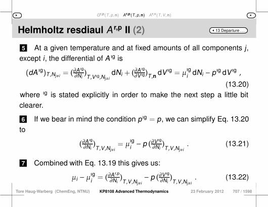
Gr,p(T ,p,n) Ar,p(T ,p,n) Ar,v(T ,V ,n)
13 Departure . . .Helmholtz resdiaul A r,p II (2)
5 At a given temperature and at fixed amounts of all components j,except i, the differential of A ıg is
(dA ıg)T ,Nj,i =(∂A ıg
∂Ni
)T ,V ıg,Nj,i
dNi +(∂A ıg
∂V ıg
)T ,n dV ıg = µıg
i dNi − pıg dV ıg ,
(13.20)where ıg is stated explicitly in order to make the next step a little bitclearer.
6 If we bear in mind the condition pıg = p, we can simplify Eq. 13.20to
(∂A ıg
∂Ni
)T ,V ,Nj,i
= µıgi − p
(∂V ıg
∂Ni
)T ,V ,Nj,i
. (13.21)
7 Combined with Eq. 13.19 this gives us:
µi − µıgi =
(∂A r,p
∂Ni
)T ,V ,Nj,i
− p(∂V ıg
∂Ni
)T ,V ,Nj,i
. (13.22)
Tore Haug-Warberg (ChemEng, NTNU) KP8108 Advanced Thermodynamics 23 February 2012 707 / 1598
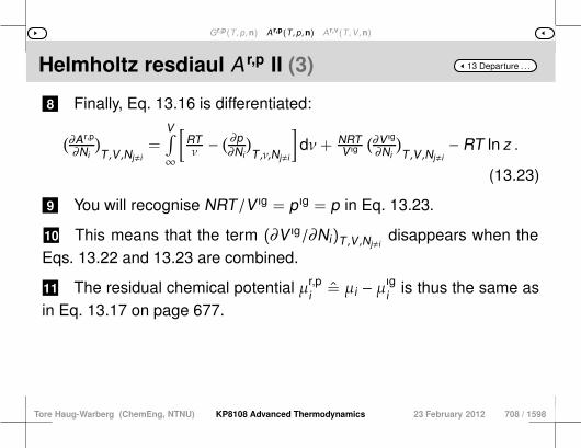
Gr,p(T ,p,n) Ar,p(T ,p,n) Ar,v(T ,V ,n)
13 Departure . . .Helmholtz resdiaul A r,p II (3)
8 Finally, Eq. 13.16 is differentiated:
(∂A r,p
∂Ni
)T ,V ,Nj,i
=V∫∞
[RTν −
( ∂p∂Ni
)T ,ν,Nj,i
]dν+ NRT
V ıg
(∂V ıg
∂Ni
)T ,V ,Nj,i
− RT ln z .
(13.23)
9 You will recognise NRT/V ıg = pıg = p in Eq. 13.23.
10 This means that the term (∂V ıg/∂Ni)T ,V ,Nj,idisappears when the
Eqs. 13.22 and 13.23 are combined.
11 The residual chemical potential µr,pi = µi − µıg
i is thus the same asin Eq. 13.17 on page 677.
Tore Haug-Warberg (ChemEng, NTNU) KP8108 Advanced Thermodynamics 23 February 2012 708 / 1598
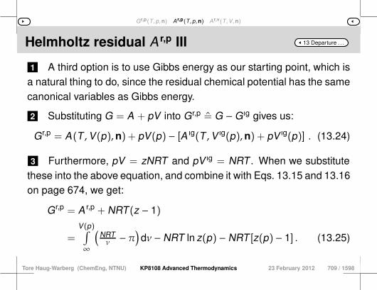
Gr,p(T ,p,n) Ar,p(T ,p,n) Ar,v(T ,V ,n)
13 Departure . . .Helmholtz residual A r,p III
1 A third option is to use Gibbs energy as our starting point, which isa natural thing to do, since the residual chemical potential has the samecanonical variables as Gibbs energy.
2 Substituting G = A + pV into Gr,p = G −Gıg gives us:
Gr,p = A(T ,V(p),n) + pV(p) − [A ıg(T ,V ıg(p),n) + pV ıg(p)] . (13.24)
3 Furthermore, pV = zNRT and pV ıg = NRT . When we substitutethese into the above equation, and combine it with Eqs. 13.15 and 13.16on page 674, we get:
Gr,p = A r,p + NRT(z − 1)
=V(p)∫∞
(NRTν − π
)dν − NRT ln z(p) − NRT [z(p) − 1] . (13.25)
Tore Haug-Warberg (ChemEng, NTNU) KP8108 Advanced Thermodynamics 23 February 2012 709 / 1598
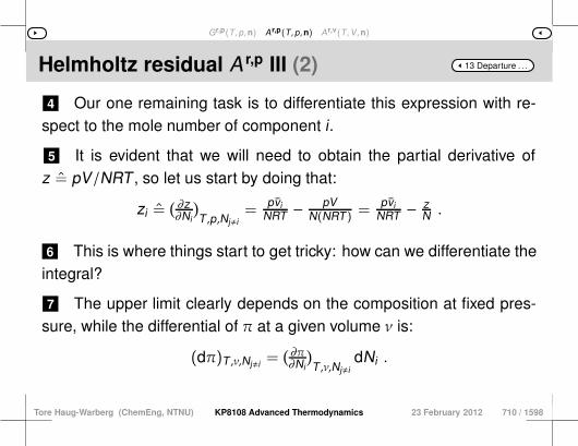
Gr,p(T ,p,n) Ar,p(T ,p,n) Ar,v(T ,V ,n)
13 Departure . . .Helmholtz residual A r,p III (2)
4 Our one remaining task is to differentiate this expression with re-spect to the mole number of component i.
5 It is evident that we will need to obtain the partial derivative ofz = pV/NRT , so let us start by doing that:
zi =( ∂z∂Ni
)T ,p,Nj,i
=pvi
NRT −pV
N(NRT) =pvi
NRT − zN .
6 This is where things start to get tricky: how can we differentiate theintegral?
7 The upper limit clearly depends on the composition at fixed pres-sure, while the differential of π at a given volume ν is:
(dπ)T ,ν,Nj,i =( ∂π∂Ni
)T ,ν,Nj,i
dNi .
Tore Haug-Warberg (ChemEng, NTNU) KP8108 Advanced Thermodynamics 23 February 2012 710 / 1598
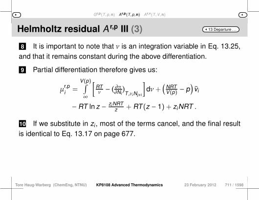
Gr,p(T ,p,n) Ar,p(T ,p,n) Ar,v(T ,V ,n)
13 Departure . . .Helmholtz residual A r,p III (3)
8 It is important to note that ν is an integration variable in Eq. 13.25,and that it remains constant during the above differentiation.
9 Partial differentiation therefore gives us:
µr,pi =
V(p)∫∞
[RTν −
( ∂π∂Ni
)T ,ν,Nj,i
]dν+
(NRTV(p) − p
)vi
− RT ln z − ziNRTz + RT(z − 1) + ziNRT .
10 If we substitute in zi , most of the terms cancel, and the final resultis identical to Eq. 13.17 on page 677.
Tore Haug-Warberg (ChemEng, NTNU) KP8108 Advanced Thermodynamics 23 February 2012 711 / 1598

Gr,p(T ,p,n) Ar,p(T ,p,n) Ar,v(T ,V ,n)
13 Departure . . .§ 108 § 107 § 109
Show that Gr,p,2.vır = NRT(z−1) = Bp when pV2.vır = NRT+Bp.
Tore Haug-Warberg (ChemEng, NTNU) KP8108 Advanced Thermodynamics 23 February 2012 712 / 1598

Gr,p(T ,p,n) Ar,p(T ,p,n) Ar,v(T ,V ,n)
13 Departure . . .§ 108 Virial Gibbs energy II
1 From Eq. 13.25 we know the general expression Gr,p = A r,p +
NRT(z − 1).
2 Combined with A r,p,2.vır = 0 from Eq. 13.18 on page 680 this givesus Gr,p,2.vır = NRT(z − 1).
3 Substituting in z2.vır = 1 + Bp/NRT gives Gr,p,2.vır = Bp in accor-dance with Eq. 13.14 on page 671.
4 The results from the various sections are thus internally consistent.
Tore Haug-Warberg (ChemEng, NTNU) KP8108 Advanced Thermodynamics 23 February 2012 713 / 1598
Gr,p(T ,p,n) Ar,p(T ,p,n) Ar,v(T ,V ,n)
13 Departure . . .(T , p,n) vs (T ,V ,n)
1 The problems we experienced in the previous section were causedby the disastrous decision to use pressure as a free variable in theHelmholtz function.
2 If we redefine the residual Helmholtz energy as
A r,v(T ,V ,n) = A(T ,V ,n)− A ıg(T ,V ,n)
we are back into the world of canonical variables, and we can use thesame approach as the one used for residual Gibbs energy on page 663.
Tore Haug-Warberg (ChemEng, NTNU) KP8108 Advanced Thermodynamics 23 February 2012 714 / 1598
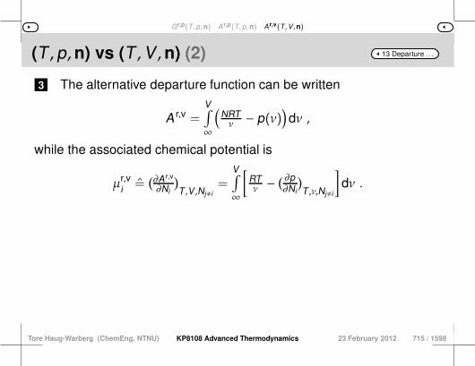
Gr,p(T ,p,n) Ar,p(T ,p,n) Ar,v(T ,V ,n)
13 Departure . . .(T , p,n) vs (T ,V ,n) (2)
3 The alternative departure function can be written
A r,v =V∫∞
(NRTν − p(ν)
)dν ,
while the associated chemical potential is
µr,vi =
(∂A r,v
∂Ni
)T ,V ,Nj,i
=V∫∞
[RTν −
( ∂p∂Ni
)T ,ν,Nj,i
]dν .
Tore Haug-Warberg (ChemEng, NTNU) KP8108 Advanced Thermodynamics 23 February 2012 715 / 1598

Gr,p(T ,p,n) Ar,p(T ,p,n) Ar,v(T ,V ,n)
13 Departure . . .§ 109 § 108 § 110
Derive an expression for A r,v and the first derivatives∂A r,v/∂(T ,V ,n) for a fluid that conforms to the Redlich–
Kwong equation of state pRK = RT/(v−b)−a/√
Tv (v + b).Use the mixing rules b(x) =
∑i bixi and a(x) =
∑i∑
j√
aiaj
xixj where bi and ai are component-specific parameters.Finally, state bi and ai as functions of Tc and pc; also
see Paragraph 46 on page 319.
Tore Haug-Warberg (ChemEng, NTNU) KP8108 Advanced Thermodynamics 23 February 2012 716 / 1598
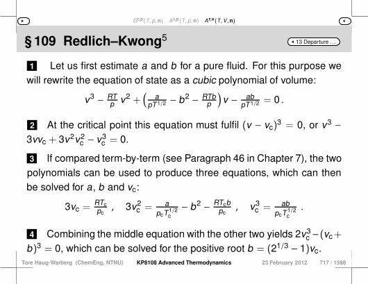
Gr,p(T ,p,n) Ar,p(T ,p,n) Ar,v(T ,V ,n)
13 Departure . . .§ 109 Redlich–Kwong5
1 Let us first estimate a and b for a pure fluid. For this purpose wewill rewrite the equation of state as a cubic polynomial of volume:
v3 − RTp v2 +
(a
pT1/2 − b2 − RTbp
)v − ab
pT1/2 = 0 .
2 At the critical point this equation must fulfil (v − vc)3 = 0, or v3 −
3vvc + 3v2v2c − v3
c = 0.
3 If compared term-by-term (see Paragraph 46 in Chapter 7), the twopolynomials can be used to produce three equations, which can thenbe solved for a, b and vc:
3vc = RTcpc
, 3v2c = a
pcT1/2c− b2 − RTcb
pc, v3
c = abpcT1/2
c.
4 Combining the middle equation with the other two yields 2v3c −(vc+
b)3 = 0, which can be solved for the positive root b = (21/3 − 1)vc.Tore Haug-Warberg (ChemEng, NTNU) KP8108 Advanced Thermodynamics 23 February 2012 717 / 1598
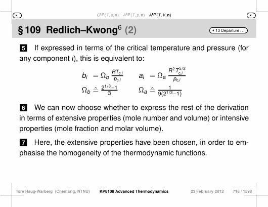
Gr,p(T ,p,n) Ar,p(T ,p,n) Ar,v(T ,V ,n)
13 Departure . . .§ 109 Redlich–Kwong6 (2)
5 If expressed in terms of the critical temperature and pressure (forany component i), this is equivalent to:
bi = ΩbRTc,ipc,i
ai = ΩaR2T5/2
c,ipc,i
Ωb = 21/3−13 Ωa = 1
9(21/3−1)
6 We can now choose whether to express the rest of the derivationin terms of extensive properties (mole number and volume) or intensiveproperties (mole fraction and molar volume).
7 Here, the extensive properties have been chosen, in order to em-phasise the homogeneity of the thermodynamic functions.
Tore Haug-Warberg (ChemEng, NTNU) KP8108 Advanced Thermodynamics 23 February 2012 718 / 1598
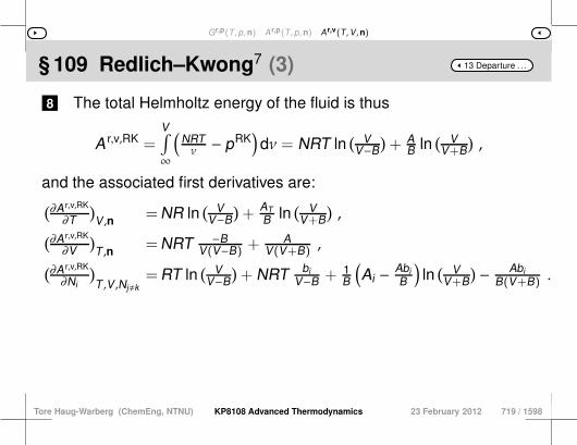
Gr,p(T ,p,n) Ar,p(T ,p,n) Ar,v(T ,V ,n)
13 Departure . . .§ 109 Redlich–Kwong7 (3)
8 The total Helmholtz energy of the fluid is thus
A r,v,RK =V∫∞
(NRTν − pRK
)dν = NRT ln
( VV−B
)+ A
B ln( VV+B
),
and the associated first derivatives are:(∂A r,v,RK
∂T)V ,n =NR ln
( VV−B
)+ AT
B ln( VV+B
),
(∂A r,v,RK
∂V)T ,n =NRT −B
V(V−B) +A
V(V+B) ,(∂A r,v,RK
∂Ni
)T ,V ,Nj,k
=RT ln( VV−B
)+ NRT bi
V−B + 1B
(Ai − Abi
B
)ln
( VV+B
) − AbiB(V+B) .
Tore Haug-Warberg (ChemEng, NTNU) KP8108 Advanced Thermodynamics 23 February 2012 719 / 1598

Gr,p(T ,p,n) Ar,p(T ,p,n) Ar,v(T ,V ,n)
13 Departure . . .§ 109 Redlich–Kwong8 (4)
9 The coefficients of the equation are defined below (note that αi hasthe same units as aVdW
i ):
B =∑i
biNi ,
A =∑i
∑j
(aiaj
T)1/2
NiNj =(∑
iα1/2
i Ni
)2,
AT = − A2T ,
Ai = 2α1/2i
∑jα1/2
j Nj = 2(αiA)1/2 ,
αi = aiT1/2
4 Otto Redlich and J. N. S. Kwong. Chem. Rev. (Washington, D. C.), 44:233–244,1949.
Tore Haug-Warberg (ChemEng, NTNU) KP8108 Advanced Thermodynamics 23 February 2012 720 / 1598

Saturation pressure Saturation volume Enthalpy of vaporization Critical exponents Maxwell equal area rule
Part 14
Simple vapour–liquid equilibrium
see also Part-Contents
Tore Haug-Warberg (ChemEng, NTNU) KP8108 Advanced Thermodynamics 23 February 2012 721 / 1598
Saturation pressure Saturation volume Enthalpy of vaporization Critical exponents Maxwell equal area rule
Contents
1 Saturation pressure
2 Saturation volume
3 Enthalpy of vaporization
4 Critical exponents
5 Maxwell equal area rule
Tore Haug-Warberg (ChemEng, NTNU) KP8108 Advanced Thermodynamics 23 February 2012 722 / 1598
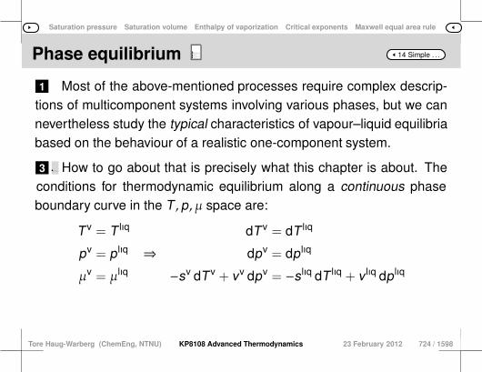
Saturation pressure Saturation volume Enthalpy of vaporization Critical exponents Maxwell equal area rule
14 Simple . . .Phase equilibrium Perspective1 In the chemical industry, vapour–liquid equilibria are essential to
the design and operation of distillation and absorption columns, oil andgas separators, evaporators and other process equipment.
2 In our everyday lives, the same physical properties cause the evap-oration of solvents in paints and varnishes, allow us to enjoy the aro-mas of wines, cheeses and coffees, make it possible to use propaneand butane in camping gas stoves, etc.
3 Moreover, at a global level, all life on Earth is inextricably linked tothe transport of water (as vapour) from warmer to cooler parts of theglobe, where it then condenses as rain or snow.
4 Although this cycle, which is driven by the sun, occurs under near-equilibrium conditions, it is responsible for the vast majority of masstransport at or near the Earth’s surface.
5 It is therefore not true to say that near-equilibrium processes are“slower” or in any way less important than irreversible processes.
723 / 1598
1 Most of the above-mentioned processes require complex descrip-tions of multicomponent systems involving various phases, but we cannevertheless study the typical characteristics of vapour–liquid equilibriabased on the behaviour of a realistic one-component system.
3 2 This makes the equations that we need to solve far simpler, be-cause they do not need to take into account the composition, and tosome extent you would expect there to be analytical solutions to theequilibrium equations. How to go about that is precisely what this chapter is about. The
conditions for thermodynamic equilibrium along a continuous phaseboundary curve in the T , p, µ space are:
T v = T lıq dT v = dT lıq
pv = p lıq ⇒ dpv = dp lıq
µv = µlıq −sv dT v + vv dpv = −s lıq dT lıq + v lıq dp lıq
Tore Haug-Warberg (ChemEng, NTNU) KP8108 Advanced Thermodynamics 23 February 2012 724 / 1598
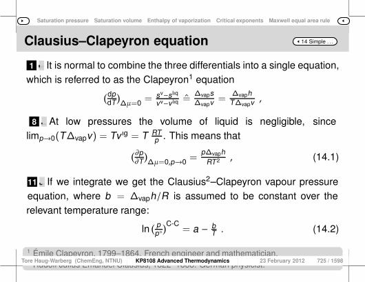
Saturation pressure Saturation volume Enthalpy of vaporization Critical exponents Maxwell equal area rule
14 Simple . . .Clausius–Clapeyron equation
1 2 The criteria on the left-hand side must be fulfilled at all equilibriumpoints, but from Section 39 on page 214 we know that the intensivestatea
3 of the system can be determinied when two of the three state vari-ables T , p, µ are known.4 Consequently, the equilibrium state can be parametrised by T , p or
T , µ or p, µ, the first of which is the most common choice.5 For a small change in the variables, the conditions on the right-
hand side then apply.
a We have not formulated a mass balance for the equilibrium, so the phase distribu-tion is unknown, but that is irrelevant in this context because (∂µ/∂N)T ,p = 0 for allone-component systems, i.e. the equilibrium is the same regardless of the quantity ofvapour and liquid. It is normal to combine the three differentials into a single equation,
which is referred to as the Clapeyron1 equation(dpdT
)∆µ=0 = sv−s lıq
vv−v lıq =∆vaps∆vapv =
∆vaphT∆vapv ,
8 6 This equation brings together four important quantities in phasetheory: vapour pressure, temperature, heat of vaporization and satura-tion volume.7 Note that the relationship between the entropy and enthalpy of va-
porization follows from the equilibrium condition ∆vapµ = 0, which sub-stituted into µ = h − Ts gives us ∆vaps = ∆vaph/T . At low pressures the volume of liquid is negligible, since
limp→0(T∆vapv) = Tv ıg = T RTp . This means that
(∂p∂T
)∆µ=0,p→0 =
p∆vaphRT2 , (14.1)
11 9 where the derivative on the left-hand side has been replaced by apartial differential (this is possible because there is only one degree offreedom in the expression).10 Let us rewrite the equation in such a way that the right-hand side becomes a weak(er) function of temperature:(∂ ln p/∂ 1
T )∆µ=0,p→0 = −∆vaphR . If we integrate we get the Clausius2–Clapeyron vapour pressure
equation, where b = ∆vaph/R is assumed to be constant over therelevant temperature range:
ln( pp)C-C
= a − bT . (14.2)
1 Émile Clapeyron, 1799–1864. French engineer and mathematician.2 Rudolf Julius Emanuel Clausius, 1822–1888. German physicist.
Tore Haug-Warberg (ChemEng, NTNU) KP8108 Advanced Thermodynamics 23 February 2012 725 / 1598

Saturation pressure Saturation volume Enthalpy of vaporization Critical exponents Maxwell equal area rule
14 Simple . . .Measured vapour pressure
1 If p ≫ 0 then we cannot assume ideal gas behaviour, and if p → pc
then the volume of liquid is no longer negligible. This undermines thetheoretical
1 1.2 1.4−3
−2
−1
0
1
1/Tr
lnp r
Figure 14.1: Vapour pressure of CO2, where is the measured value and ×is the deviation.
Tore Haug-Warberg (ChemEng, NTNU) KP8108 Advanced Thermodynamics 23 February 2012 726 / 1598
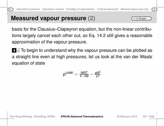
Saturation pressure Saturation volume Enthalpy of vaporization Critical exponents Maxwell equal area rule
14 Simple . . .Measured vapour pressure (2)
basis for the Clausius–Clapeyron equation, but the non-linear contribu-tions largely cancel each other out, so Eq. 14.2 still gives a reasonableapproximation of the vapour pressure.
4 2 This relationship is illustrated in Figure 14.1, which shows a vapourpressure curve that is surprisingly rectilinear, even close to the criticalpoint (cf. Matlab-program 30:1.11).3 The percentage difference between the calculated and measured
vapour pressurea is given by ×.
a W. Duschek, R. Kleinrahm, and W. Wagner. J. Chem. Thermodynamics, 22:841–864, 1990. To begin to understand why the vapour pressure can be plotted as
a straight line even at high pressures, let us look at the van der Waalsequation of state
pVdW = NRTV−Nb − aN2
V2
Tore Haug-Warberg (ChemEng, NTNU) KP8108 Advanced Thermodynamics 23 February 2012 727 / 1598
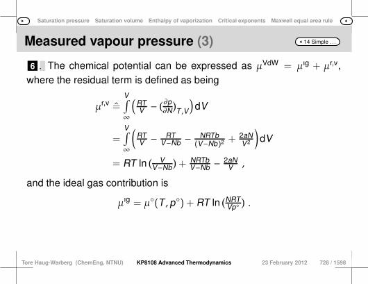
Saturation pressure Saturation volume Enthalpy of vaporization Critical exponents Maxwell equal area rule
14 Simple . . .Measured vapour pressure (3)
6 5 in greater detail. The chemical potential can be expressed as µVdW = µıg + µr,v,where the residual term is defined as being
µr,v =V∫∞
(RTV −
(∂p∂N
)T ,V
)dV
=V∫∞
(RTV − RT
V−Nb − NRTb(V−Nb)2 + 2aN
V2
)dV
= RT ln( VV−Nb
)+ NRTb
V−Nb − 2aNV ,
and the ideal gas contribution is
µıg = µ(T , p) + RT ln(NRT
Vp).
Tore Haug-Warberg (ChemEng, NTNU) KP8108 Advanced Thermodynamics 23 February 2012 728 / 1598
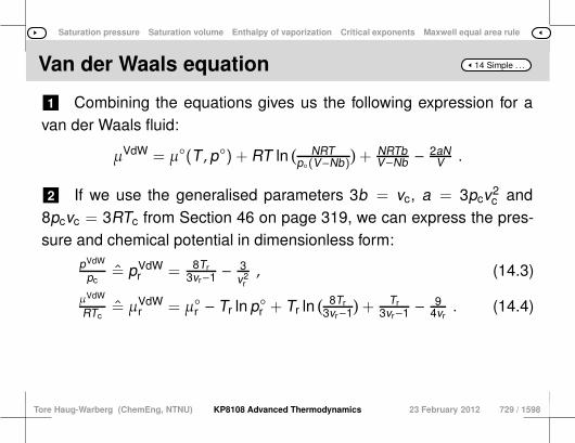
Saturation pressure Saturation volume Enthalpy of vaporization Critical exponents Maxwell equal area rule
14 Simple . . .Van der Waals equation
1 Combining the equations gives us the following expression for avan der Waals fluid:
µVdW = µ(T , p) + RT ln( NRTp(V−Nb)
)+ NRTb
V−Nb − 2aNV .
2 If we use the generalised parameters 3b = vc, a = 3pcv2c and
8pcvc = 3RTc from Section 46 on page 319, we can express the pres-sure and chemical potential in dimensionless form:
pVdW
pc= pVdW
r = 8Tr3vr−1 − 3
v2r, (14.3)
µVdW
RTc= µVdW
r = µr − Tr ln pr + Tr ln( 8Tr3vr−1
)+ Tr
3vr−1 − 94vr
. (14.4)
Tore Haug-Warberg (ChemEng, NTNU) KP8108 Advanced Thermodynamics 23 February 2012 729 / 1598

Saturation pressure Saturation volume Enthalpy of vaporization Critical exponents Maxwell equal area rule
14 Simple . . .Van der Waals A
1 It is worth noting that these two equations represent a complete setof equations of state for Helmholtz energy.
2 Integration using the Euler method gives us A = −pV + µN, whichexpressed in dimensionless form becomes A
NRTc= − pV
NRTc+
µRTc
. Rewrit-ing this in reduced variables:
aVdWr = AVdW
NRTc= − 3
8 pVdWr vr + µVdW
r (14.5)
3 since the critical compressibility factor is zc = pcvc/RTc = 38 for the
van der Waals equation of state.
Tore Haug-Warberg (ChemEng, NTNU) KP8108 Advanced Thermodynamics 23 February 2012 730 / 1598
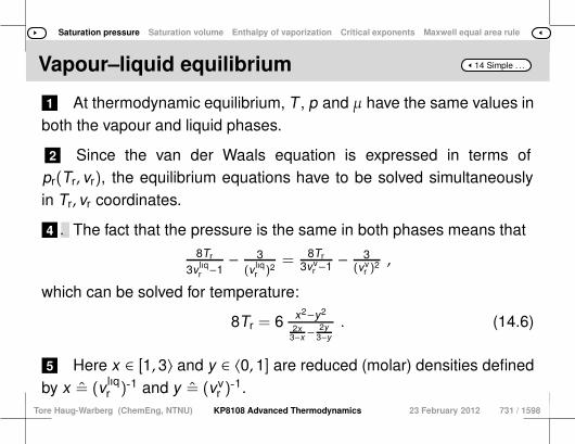
Saturation pressure Saturation volume Enthalpy of vaporization Critical exponents Maxwell equal area rule
14 Simple . . .Vapour–liquid equilibrium
1 At thermodynamic equilibrium, T , p and µ have the same values inboth the vapour and liquid phases.
2 Since the van der Waals equation is expressed in terms ofpr(Tr, vr), the equilibrium equations have to be solved simultaneouslyin Tr, vr coordinates.
4 3 We can’t expect there to be an analytical solution to this problem,but there is no harm in setting out the equations. The fact that the pressure is the same in both phases means that
8Tr
3v lıqr −1− 3
(v lıqr )2
= 8Tr3vv
r −1 −3
(vvr )
2 ,
which can be solved for temperature:
8Tr = 6 x2−y2
2x3−x −
2y3−y
. (14.6)
5 Here x ∈ [1, 3〉 and y ∈ 〈0, 1] are reduced (molar) densities definedby x = (v lıq
r )-1 and y = (vvr )
-1.Tore Haug-Warberg (ChemEng, NTNU) KP8108 Advanced Thermodynamics 23 February 2012 731 / 1598
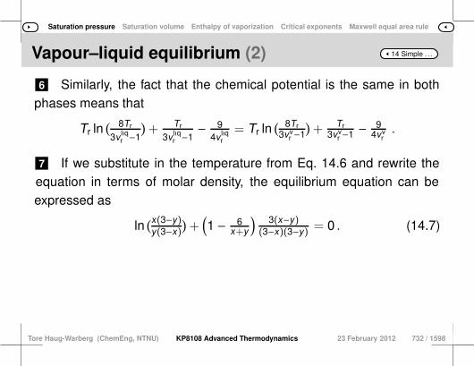
Saturation pressure Saturation volume Enthalpy of vaporization Critical exponents Maxwell equal area rule
14 Simple . . .Vapour–liquid equilibrium (2)
6 Similarly, the fact that the chemical potential is the same in bothphases means that
Tr ln( 8Tr
3v lıqr −1
)+ Tr
3v lıqr −1− 9
4v lıqr
= Tr ln( 8Tr3vv
r −1
)+ Tr
3vvr −1 −
94vv
r.
7 If we substitute in the temperature from Eq. 14.6 and rewrite theequation in terms of molar density, the equilibrium equation can beexpressed as
ln(x(3−y)y(3−x)
)+
(1 − 6
x+y
)3(x−y)
(3−x)(3−y) = 0 . (14.7)
Tore Haug-Warberg (ChemEng, NTNU) KP8108 Advanced Thermodynamics 23 February 2012 732 / 1598

Saturation pressure Saturation volume Enthalpy of vaporization Critical exponents Maxwell equal area rule
14 Simple . . .Pressure–potential diagram
1 In order to determine the saturation state of the fluid, we need tosolve Eq. 14.7 for y = y(x) or x = x(y).
3 2 The latter was used in the Matlab function 30:2.5, which calculatesx ∈ [1, 3〉 for a given value of y ∈ 〈0, 1]. The solution is shown graphically in Figure 14.2 on the next page
along with a parametrised pr(vr), µr(vr) diagram3.
6 4 Here the simultaneous solution of p lıqr = pv
r and µlıqr = µv
r appearsas the triple point of a manifold with three regions (vapour, liquid and anunphysical fluid phase for which (∂p/∂v)T > 0).5 The figures were drawn using the Matlab program 30:1.10. Note that the slope of the graph asymptotically approaches −1 as
it nears the critical point, where xc = yc = 1. 7 This means that one of the densities decreases at the same rateas the other one increases in the two-phase region i.e. for Tr < 1. The average density of
the two phases therefore has the constant value 12 (x + y) ≃ 1.
8 Experimentally it has been demonstrated that the value of x + y isnot quite constant, but nevertheless it is virtually a linear function of Tr
(hence it is also referred to as the rectilinear density) over a wide rangeof temperatures.9 This is as far as we can get by looking at the general case, so we
will now move on to a discussion of the asymptotes of the graph.
3 The volume increases from the top right corner down to the bottom left corner of thefigure.
Tore Haug-Warberg (ChemEng, NTNU) KP8108 Advanced Thermodynamics 23 February 2012 733 / 1598

Saturation pressure Saturation volume Enthalpy of vaporization Critical exponents Maxwell equal area rule
0 0.5 11
1.5
2
2.5
3
−1 0 1 2−1
0
1
2
3
Molar density
ρvr
ρlıq r
Pressure–chem.pot.
pr
µr
c.p.
Figure 14.2: ρvr , ρ
lıqr saturation graph, with the associated isotherms, ex-
pressed in pr, µr coordinates (drawn with volume as the parameter).
Tore Haug-Warberg (ChemEng, NTNU) KP8108 Advanced Thermodynamics 23 February 2012 734 / 1598
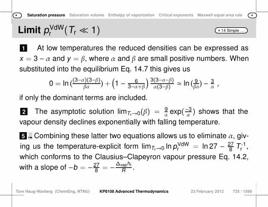
Saturation pressure Saturation volume Enthalpy of vaporization Critical exponents Maxwell equal area rule
14 Simple . . .Limit pVdWr (Tr ≪ 1)
1 At low temperatures the reduced densities can be expressed asx = 3 − α and y = β, where α and β are small positive numbers. Whensubstituted into the equilibrium Eq. 14.7 this gives us
0 = ln((3−α)(3−β)
βα
)+
(1 − 6
3−α+β) 3(3−α−β)
α(3−β) ≃ ln( 9βα
) − 3α ,
if only the dominant terms are included.
2 The asymptotic solution limTr→0(β) = 9α exp(−3
α ) shows that thevapour density declines exponentially with falling temperature.
5 3 In that limit case, the temperature Eq. 14.6 can be expressed as
limTr→0
(8TVdWr ) = 6 (3−α)2−(β)2
2(3−α)α − 2β
3−β≃ 9α ,
4 and if we substitute that into the van der Waals equation we get
limTr→0
pVdWr = 8Tr
3β−1 − 3β2 ≃ 9αα3 exp( 3α)−1 ≃
27exp( 3α)
. Combining these latter two equations allows us to eliminate α, giv-ing us the temperature-explicit form limTr→0 ln pVdW
r = ln 27 − 278 T -1
r ,which conforms to the Clausius–Clapeyron vapour pressure Eq. 14.2,with a slope of −b = −27
8 = −∆vaphr
R .
Tore Haug-Warberg (ChemEng, NTNU) KP8108 Advanced Thermodynamics 23 February 2012 735 / 1598

Saturation pressure Saturation volume Enthalpy of vaporization Critical exponents Maxwell equal area rule
14 Simple . . .Limit pVdWr (Tr → 1)
1 Near the critical point, the reduced densities can be expressed asx = 1 + α and y = 1 − β, where α and β are small positive numbers. Ifwe substitute these values into the equilibrium Eq. 14.7 we get
ln((1+α)(2+β)(1−β)(2−α)
)+
(1 − 6
2+α−β) 3(α+β)(2−α)(2+β) = 0 .
3 2 Now let us expand ln(1+x) = x +O(x2) and multiply out the termsin brackets. We can ignore all higher order terms of the kind αβ, α2 and β2:
0 = α+ 12 β − (−β − 1
2 α) +(1 − 6
2+α−β) 3(α+β)
4+2β−2α−αβ
≃ 1 +(1 − 6
2+α−β)
12+β−α
= 4 − (β − α)2 + 2 + (β − α) − 6
≃ β − α . (14.8)
Tore Haug-Warberg (ChemEng, NTNU) KP8108 Advanced Thermodynamics 23 February 2012 736 / 1598
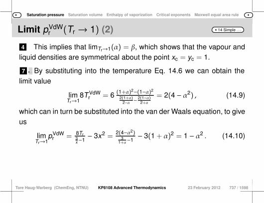
Saturation pressure Saturation volume Enthalpy of vaporization Critical exponents Maxwell equal area rule
14 Simple . . .Limit pVdWr (Tr → 1) (2)
4 This implies that limTr→1(α) = β, which shows that the vapour andliquid densities are symmetrical about the point xc = yc = 1.
7 5 This is an important results, which has also been confirmed exper-imentallyab,6 see Figure 14.3 on page 714 (cf. Matlab-program 30:1.11).
a The critical volume of a fluid can be estimated using straight-line extrapolation of thesub-critical vapour and liquid densities, while the critical pressure and temperature canbe measured directly.b Molar entropy displays a similar symmetry; see Figure 18.9 on page 996. By substituting into the temperature Eq. 14.6 we can obtain the
limit value
limTr→1
8TVdWr = 6 (1+α)2−(1−α)2
2(1+α)2−α −
2(1−α)2+α
= 2(4 − α2) , (14.9)
which can in turn be substituted into the van der Waals equation, to giveus
limTr→1
pVdWr = 8Tr
3x−1− 3x2 =
2(4−α2)3
1+α−1− 3(1 + α)2 = 1 − α2 . (14.10)
Tore Haug-Warberg (ChemEng, NTNU) KP8108 Advanced Thermodynamics 23 February 2012 737 / 1598

Saturation pressure Saturation volume Enthalpy of vaporization Critical exponents Maxwell equal area rule
14 Simple . . .Limit pVdWr (Tr → 1) (3)
8 Here we should note that both TVdWr and pVdW
r are simple functionsof α2.9 In other words, the phase envelope is parabolic with the critical
point as its origin. If α2 is eliminated from the last two equations, the saturation pressurecan instead be written as a logarithmic function with temperature as itsfree variable:
limTr→1
ln(pVdWr ) = ln(4Tr − 3) ≃ 4(Tr − 1) .
10 If we combine this with the Clausius–Clapeyron vapour pressureEq. 14.2 we get the slope limTr→1 ∂ ln pr/∂(1/T) = −4T2
r ≥ −4.
Tore Haug-Warberg (ChemEng, NTNU) KP8108 Advanced Thermodynamics 23 February 2012 738 / 1598

Saturation pressure Saturation volume Enthalpy of vaporization Critical exponents Maxwell equal area rule
14 Simple . . .Vapour pressure curve
1 The conclusion is that the slope of the vapour pressure curve variesin the range −4 < −b < − 27
8 .
3 2 At the small scale of Figure 14.1 this variation is hardly noticeableand ln(pVdW
r ) = f(1/T) appears to be a straight line. The van der Waals equation therefore gives us a qualitatively ac-curate representation of the vapour pressure curve, although from ex-perience we know that the model is insufficiently accurate for quantita-tive purposes.
5 4 It would be unreasonable to expect otherwise — it is impossible fortwo parameters to fully describe all of the thermodynamic systems inthe world. The one-phase region is not adequately represented either, but
once again it is qualitatively accurate, as seen in Figure 14.34.6 As such, only small changes are needed to improve the predictiveaccuracy.7 In 1949, Redlich and Kwonga introduced the first improvement by
making the a term temperature-dependent.8 Since then, a number of related equations of state have been pub-
lishedbc, but they are all cubicd
9 functions of the volume (or density), and their qualitative propertiesare the same.10 This means that the van der Waals equation of state still remainsan important conceptual model — 140 years after it was formulated.
a Otto Redlich and J. N. S. Kwong. Chem. Rev. (Washington, D. C.), 44:233–244,1949.b Giorgio Soave. Fluid Phase Equilib., pages 1197–1203, 1972.c Ding-Yu Peng and Donald B. Robinson. Ind. Eng. Chem. Fundam., 15(1):59–64,1976.d There are now around a hundred closely related models, with the Redlich–Kwong–Soave and Peng–Robinson (PR) models being two of the best-known ones.
4 W. Duschek, R. Kleinrahm, and W. Wagner. J. Chem. Thermodynamics, 22:841–864, 1990.
Tore Haug-Warberg (ChemEng, NTNU) KP8108 Advanced Thermodynamics 23 February 2012 739 / 1598
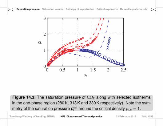
Saturation pressure Saturation volume Enthalpy of vaporization Critical exponents Maxwell equal area rule
0 0.5 1 1.5 2 2.50
1
2
3
ρr
p r
Figure 14.3: The saturation pressure of CO2 along with selected isothermsin the one-phase region (280 K, 313 K and 330 K respectively). Note the sym-metry of the saturation pressure psat
r around the critical density ρr ,c = 1.
Tore Haug-Warberg (ChemEng, NTNU) KP8108 Advanced Thermodynamics 23 February 2012 740 / 1598
Saturation pressure Saturation volume Enthalpy of vaporization Critical exponents Maxwell equal area rule
14 Simple . . .Critical phenomena
1 At sufficiently low temperatures, the molar density of a liquid ap-proaches a constant value of limTr→0(x) = 3.
2 As the temperature increases, the liquid phase gradually becomesless significant, until it ceases to exist entirely at the critical point wherelimTr→1(x) = limTr→1(y) = 1.
3 In this state there is no fundamental difference between a gas anda liquid.
4 This idea is supported by Eq. 14.8, which shows that the densityof the two phases is symmetrical about xc = yc = 1 close to the criticalpoint.
Tore Haug-Warberg (ChemEng, NTNU) KP8108 Advanced Thermodynamics 23 February 2012 741 / 1598
Saturation pressure Saturation volume Enthalpy of vaporization Critical exponents Maxwell equal area rule
14 Simple . . .Limit vVdWr (Tr ≪ 1)
1 As previously mentioned, when the temperature approaches zero,the specific volume of the liquid tends to a ratio of limTr→0(vVdW
r ) = 13 .
Tore Haug-Warberg (ChemEng, NTNU) KP8108 Advanced Thermodynamics 23 February 2012 742 / 1598

Saturation pressure Saturation volume Enthalpy of vaporization Critical exponents Maxwell equal area rule
14 Simple . . .Limit vVdWr (Tr → 1)
1 Close to the critical point, the reduced density of the liquid can beexpressed as x = (v lıq
r )-1 = 1 + α where α is a small number, and fromEq. 14.9 we can then derive the asymptotic temperature function:
limTr→1
(v lıqr )VdW = lim
Tr→1
11+α = 1
1+√
4−4Tr≃ 1 − 2
√1 − Tr .
2 This makes the logarithm of the saturation volume
limTr→1
ln(v lıqr )VdW ≃ −2
√1 − Tr ,
3 while the Racketta equation, which forms the basis for several semi-empirical correlations, states that ln(v lıq
r )Rackett = ln(zc)·(1−Tr)2/7 whereln(zc) ≈ −1.2 for nonpolar substances.4 The parameters in the two equations are different, but qualitatively
there is still a real correspondence between theory and practiceb.
a Harold G. Rackett. J. Chem. Eng. Data., 15(4):514–518, 1970.b The van der Waals equation indicates that the function should take the form a(1−Tr)b
and also gives us good initial values that can be adjusted to reflect experimental data(both the proportionality constant ln(zc) and the exponent 2/7 in the Rackett equationare empirical).
Tore Haug-Warberg (ChemEng, NTNU) KP8108 Advanced Thermodynamics 23 February 2012 743 / 1598
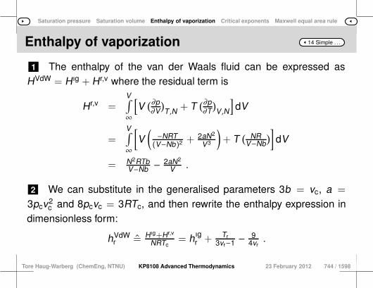
Saturation pressure Saturation volume Enthalpy of vaporization Critical exponents Maxwell equal area rule
14 Simple . . .Enthalpy of vaporization
1 The enthalpy of the van der Waals fluid can be expressed asHVdW = Hıg + Hr,v where the residual term is
Hr,v =V∫∞
[V
(∂p∂V
)T ,N + T
(∂p∂T
)V ,N
]dV
=V∫∞
[V
(−NRT
(V−Nb)2 + 2aN2
V3
)+ T
( NRV−Nb
)]dV
= N2RTbV−Nb − 2aN2
V .
2 We can substitute in the generalised parameters 3b = vc, a =
3pcv2c and 8pcvc = 3RTc, and then rewrite the enthalpy expression in
dimensionless form:
hVdWr = Hıg+Hr,v
NRTc= hıg
r + Tr3vr−1 − 9
4vr.
Tore Haug-Warberg (ChemEng, NTNU) KP8108 Advanced Thermodynamics 23 February 2012 744 / 1598
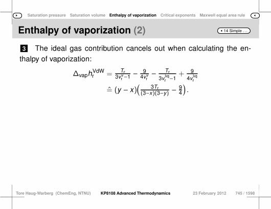
Saturation pressure Saturation volume Enthalpy of vaporization Critical exponents Maxwell equal area rule
14 Simple . . .Enthalpy of vaporization (2)
3 The ideal gas contribution cancels out when calculating the en-thalpy of vaporization:
∆vaphVdWr = Tr
3vvr −1 −
94vv
r− Tr
3v lıqr −1
+ 94v lıq
r
= (y − x)(
3Tr(3−x)(3−y) −
94
).
Tore Haug-Warberg (ChemEng, NTNU) KP8108 Advanced Thermodynamics 23 February 2012 745 / 1598
Saturation pressure Saturation volume Enthalpy of vaporization Critical exponents Maxwell equal area rule
14 Simple . . .Limit ∆vaphVdWr (Tr ≪ 1)
1 In practice, the low-temperature limit limTr→0(∆vaphVdWr ) = 27
8 cannever be reached, because most liquids freeze at a temperature ofTr ≈ 0.7. Table 14.4 on the following page therefore gives a comparisonwith the heat of vaporization5 measured at the normal boiling point.2 As can be seen from the table, the correlation between the two is
no more than reasonable.
5 Robert C. Reid, John M. Prausnitz, and Thomas K. Sherwood. The Properties ofGases and Liquids. McGraw-Hill, 3rd edition, 1977.
Tore Haug-Warberg (ChemEng, NTNU) KP8108 Advanced Thermodynamics 23 February 2012 746 / 1598

Saturation pressure Saturation volume Enthalpy of vaporization Critical exponents Maxwell equal area rule
Figure 14.4: Enthalpy of vaporization at the normal boiling point comparedwith ∆vaphVdW
r = 278 = 3.375 calculated from the van der Waals equation.
Tb[K]
Tc[K]
∆vaph[cal/mol]
∆vaphRTc
∆vaphVdW
[cal/mol]
N2 77.35 126.2 1333 5.32 846Ar 87.27 150.8 1560 5.21 1011O2 90.17 154.6 1630 5.31 1037
CH4 111.66 190.4 1955 5.17 1277Kr 119.74 209.4 2309 5.55 1404
H2O 373.15 647.3 9717 7.55 4341
Tore Haug-Warberg (ChemEng, NTNU) KP8108 Advanced Thermodynamics 23 February 2012 747 / 1598
Saturation pressure Saturation volume Enthalpy of vaporization Critical exponents Maxwell equal area rule
14 Simple . . .Limit ∆vaphVdWr (Tr → 1)
1 Close to the critical point, the reduced densities can be expressedas x = 1 + α and y = 1 − β, where α and β are small positive numbers:
∆vaphVdWr = −(α+ β)
(3Tr
(2−α)(2+β) −94
).
2 Now let us substitute in limTr→1(β) = α and limTr→1(4Tr) = 4 − α2
from Eq. 14.9:
limTr→1
∆vaphVdWr = −2α
(3Tr
4−α2 − 94
)= 6
√1 − Tr .
3 The Watsona correlation ∆vaphWatson = a(1 − Tr)b , which statesthat b ≈ 0.38 for nonpolar organic compounds, goes a long way towardsconfirming this result.
a K. M. Watson. Ind. Eng. Chem., 35:398, 1943.
Tore Haug-Warberg (ChemEng, NTNU) KP8108 Advanced Thermodynamics 23 February 2012 748 / 1598

Saturation pressure Saturation volume Enthalpy of vaporization Critical exponents Maxwell equal area rule
14 Simple . . .Critical exponents
1 In Section 48 on page 325 we showed that the van der Waals equa-tion can be written in its reduced form without the use of any arbitrarymodel parameters.
5 2 The underlying theory is based on the critical properties of the fluidunder the conditions (∂p/∂v)T = 0 and (∂2p/∂v∂v)T = 0, calculated atT = Tc and v = vc, and of course also at p = pc.3 This produces two equations that contain the two parameters a and
b.4 Conventionally, the equations are solved with respect to a and b as
functions of Tc and pc. This results in a useful form of the equation of state, which wehave used in this chapter to analyse the fluid’s behaviour in a numberof interesting limit cases.
6 Nevertheless, Figure 14.3, to give a specific example, shows thatthe theory is by no means universally applicable.
7 In this section we will look in greater detail at what happens close tothe critical point, and quantify to what extent the van der Waals equationfails to predict experimental results.
Tore Haug-Warberg (ChemEng, NTNU) KP8108 Advanced Thermodynamics 23 February 2012 749 / 1598
Saturation pressure Saturation volume Enthalpy of vaporization Critical exponents Maxwell equal area rule
14 Simple . . .Critical exponents (2)
8 It has been theoretically proven — and experimentally confirmed —that the energy surface close to the critical point of a vapour–liquidequilibrium is of a universal form, which is parametrised by what we callan order parameter.
15 9 The order parameter reflects the characteristic behaviour of thefluid in phase transitions.10 By definition it is zero at the critical point and in the surroundingone-phase region.11 In two-phase regions it gradually increases with the distance fromthe critical point.12 For reasons of symmetry, we wouldn’t expect the order parameterto differ between vapour–liquid and liquid–vapour transitions.13 There is absolutely no reason for it to do so, since there is no ther-modynamic distinction between a vapour phase and a liquid phase.14 They are both fluids. For vapour–liquid equilibria, it is natural to use
∣∣∣ρr − 1∣∣∣ as an order
parameter, provided that it produces symmetrical phase transitions6,which it indeed does.
17 16 In fact, that order parameter is precisely what explains the rectilin-ear density graph mentioned in conjunction with Figure 14.2. Outside the two-phase region (using values along the fluid’s critical
isochore moving towards the critical point) it is possible to observe agradual phase transition in the fluid.
18 The closer we get to the critical point, the more anomalous thebehaviour of the fluid.
Tore Haug-Warberg (ChemEng, NTNU) KP8108 Advanced Thermodynamics 23 February 2012 750 / 1598

Saturation pressure Saturation volume Enthalpy of vaporization Critical exponents Maxwell equal area rule
14 Simple . . .Critical exponents (3)
22 19 This is called a λ transition or a 2nd order phase transition.20 The name λ transition comes from the variation in heat capacity asa function of distance from the critical point:21 when Tr − 1 is used as the measure of distance from the criticalpoint, the shape of the graph is reminiscent of the Greek letter lambda. In the literature for this field, which incidentally covers a large and
exciting range of research7, the critical anomalies of the fluid are ex-pressed using divergence formulae:
One phase, ρr = 1 : cv ∝ (Tr − 1)−α , (14.11)
One phase, ρr = 1 :(∂ρr
∂pr
)Tr∝ (Tr − 1)−γ , (14.12)
Critical, Tr = 1 : |pr − 1| ∝ |ρr − 1| +δ , (14.13)
Two phases, Tr < 1 : |ρr − 1| ∝ (1 − Tr)+β . (14.14)
23 In the next four sections we will derive the classical values of theexponents α, γ, δ and β, based on our understanding of a van der Waalsfluid.24 However, the results that we will obtain are not only true for the vander Waals equation, they are also valid for all explicit equations of state,regardless of whether or not they are cubic.25 This is because we are only interested in the exponents in theabove equations— not the proportionality factors.26 It turns out that the exponents are the same, whether you start outfrom the van der Waals equation or from a more advanced (modern)equation of state.27 This classical theory is also known as the Landau theory.
6 The theory applies to all phase equilibria that have a single (scalar) order parameter.For example, ferromagnetic materials display relatively analogous behaviour, whichis described by the order parameter |Mr − 1|, where M is the magnetisation of thesubstance.7 Kenneth G. Wilson received the Nobel prize in 1982 for his contribution to the devel-opment of renormalisation groups applied to, amongst other things, critical phase tran-sitions.
Tore Haug-Warberg (ChemEng, NTNU) KP8108 Advanced Thermodynamics 23 February 2012 751 / 1598

Saturation pressure Saturation volume Enthalpy of vaporization Critical exponents Maxwell equal area rule
14 Simple . . .Isochoric heat capacity (α)
1 2 From our knowledge of thermodynamic theory, and particularlyfrom chapters 4 and 8 on Legendre transformations and on the ther-modynamics of systems of constant composition, we know the generalrelationships (∂A/∂T)V ,n = −S and (∂S/∂T)V ,n = CV/T .3 These equations can also be expressed in reduced coordinates as(∂ar/∂Tr)vr = −s/R and (∂s/∂Tr)vr = cv/Tr. Eliminating s gives us cv = −RTr (∂2ar/∂Tr∂Tr)vr
. In other words,the heat capacity of the fluid gives us the second derivative of Helmholtzenergy.
4 For a van der Waals fluid, we can obtain the Helmholtz energy bycombining Eq. 14.5 with equations 14.3 and 14.4.
5 Double differentiation of ar with respect to Tr gives us
cVdWv = −RTr
(( ∂2µr∂Tr∂Tr
)+ 1
Tr
)= cp − R = cv (T) .
9 6 Note that the temperature derivative of µ gives us cp rather thancv .7 This is because the standard state is defined at p, which implies
that v is a variable with respect to temperature.8 This topic is discussed more thoroughly in the context of Eq. 7.9 on
page 255. We can therefore conclude that αVdW = 0 in Eq. 14.11.10 This assumes that the heat capacity in the standard state behaves“normally” close to the critical temperature of the fluid, but this is verylikely to be the case, given that cv refers to an ideal gas state.11 After all, the critical state is a result of the non-ideal nature of thefluid, and the standard state doesn’t tell us anything about non-idealconditions.12 Although cv is a function of temperature, it does not display anytemperature divergence of the type (Tr − 1)−α.13 cv can therefore be considered a constant in this context.
Tore Haug-Warberg (ChemEng, NTNU) KP8108 Advanced Thermodynamics 23 February 2012 752 / 1598
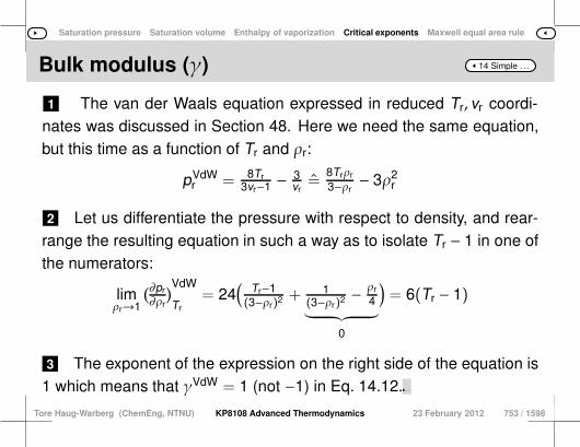
Saturation pressure Saturation volume Enthalpy of vaporization Critical exponents Maxwell equal area rule
14 Simple . . .Bulk modulus (γ)
1 The van der Waals equation expressed in reduced Tr, vr coordi-nates was discussed in Section 48. Here we need the same equation,but this time as a function of Tr and ρr:
pVdWr = 8Tr
3vr−1 − 3vr=
8Trρr
3−ρr− 3ρ2
r
2 Let us differentiate the pressure with respect to density, and rear-range the resulting equation in such a way as to isolate Tr − 1 in one ofthe numerators:
limρr→1
(∂pr∂ρr
)VdW
Tr= 24
(Tr−1
(3−ρr)2 + 1(3−ρr)2 −
ρr
4︸ ︷︷ ︸
0
)= 6(Tr − 1)
3 The exponent of the expression on the right side of the equation is1 which means that γVdW = 1 (not −1) in Eq. 14.12.4 The expression above is written for the bulk modulus while
Eq. 14.12 is valid for the isothermal compressibility.5 These are mutually resiprocal quantities which explains the sign
shift of the exponent.
Tore Haug-Warberg (ChemEng, NTNU) KP8108 Advanced Thermodynamics 23 February 2012 753 / 1598
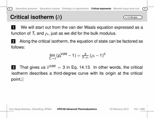
Saturation pressure Saturation volume Enthalpy of vaporization Critical exponents Maxwell equal area rule
14 Simple . . .Critical isotherm (δ)
1 We will start out from the van der Waals equation expressed as afunction of Tr and ρr, just as we did for the bulk modulus.
2 Along the critical isotherm, the equation of state can be factored asfollows:
limTr→1
(pVdWr − 1) = 3
3−ρr(ρr − 1)3
3 That gives us δVdW = 3 in Eq. 14.13. In other words, the criticalisotherm describes a third-degree curve with its origin at the criticalpoint.4 This is why the van der Waals equation and other related equations
are sometimes called “cubic equations of state”.
Tore Haug-Warberg (ChemEng, NTNU) KP8108 Advanced Thermodynamics 23 February 2012 754 / 1598
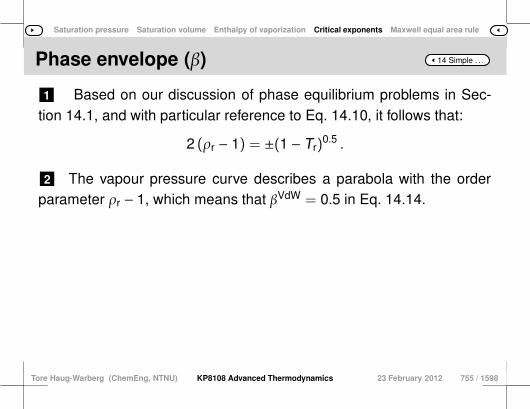
Saturation pressure Saturation volume Enthalpy of vaporization Critical exponents Maxwell equal area rule
14 Simple . . .Phase envelope (β)
1 Based on our discussion of phase equilibrium problems in Sec-tion 14.1, and with particular reference to Eq. 14.10, it follows that:
2 (ρr − 1) = ±(1 − Tr)0.5 .
2 The vapour pressure curve describes a parabola with the orderparameter ρr − 1, which means that βVdW = 0.5 in Eq. 14.14.
Tore Haug-Warberg (ChemEng, NTNU) KP8108 Advanced Thermodynamics 23 February 2012 755 / 1598

Saturation pressure Saturation volume Enthalpy of vaporization Critical exponents Maxwell equal area rule
Figure 14.5: Critical exponents measured experimentally for selected com-pounds compared with the classical values calculated from the van der Waalsequation of state.
System α γ δ β
Van der Waals 0 1 3 0.5Ising 3D 82 0.110(1) 1.237(2) 4.789(2) 0.326(5)Heisenberg 3D 92 −.1336(2) 1.3960(9) 4.783(3) 0.3689(3)Ni, Fe, Gd2BrC, Gd2IC,Tl2Mn2O7, . . . 102
−.1336(2) 1.3960(9) 4.783(3) 0.3689(3)
3 He, 4 He, Xe, CO2,H2O, O2
1120.10(0) 1.19(0) 4.35(0) 0.35(5)
122 J. M. H. Levelt Sengers and J. V. Sengers. Phys. Rev. A, 12(6):2622–2627, 1975.
Tore Haug-Warberg (ChemEng, NTNU) KP8108 Advanced Thermodynamics 23 February 2012 756 / 1598

Saturation pressure Saturation volume Enthalpy of vaporization Critical exponents Maxwell equal area rule
14 Simple . . .Critical point measurements
1 Table 14.5 gives a summary of what we have learned so far aboutphase transitions and how they relate to the van der Waals equation.
3 2 As can clearly be seen from the table, the equation of state doesnot accurately describe what happens in real life, but we knew that al-ready. What is surprising is that the experimental values do not diverge;
instead they suggest that physical quantities exhibit certain universalbehaviour during phase transitions.
8 4 Here we should note that the exponents α–δ vary surprisingly little,both in response to changes in the chemistry of the system and to thephysical properties defined by the order parameter.5 Intuitively you would expect there to be a big difference between
vapour–liquid phase transitions and ferromagnetism, but it turns out thatthe critical exponents of these phenomena are roughly the same.6 We are clearly standing at the threshold of a new understanding of
the world.7 However, the theory that underpins it is unfortunately beyond our
reach, and we will therefore have to limit ourselves to a verbal discus-sion of the topic. What we can say for sure is that there is no equation with an an-
alytical solution that accurately describes critical phenomena in nature.In other words, the critical exponents are neither integers (z ∈ Z) norsimple fractions (q ∈ Q).
13 9 That is what they would need to be for there to be any hope of find-ing an equation of state with an analytical solution capable of describ-ing phase transition behaviour.10 This is because expanding such an equation would always produceexponents that are rational numbers or integers.11 That is not the case, and we must therefore give up on trying to findan all-encompassing universal equation to describe the laws of nature.12 Our next observation is loosely related to statistical thermodynam-ics and to the knowledge that some models are easier to deal with thanothers. The simplest special case is a gas in which the molecules are con-
stantly moving around without colliding or interacting with each other inany way. That is what we mean by an ideal gas.
Tore Haug-Warberg (ChemEng, NTNU) KP8108 Advanced Thermodynamics 23 February 2012 757 / 1598
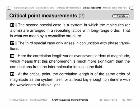
Saturation pressure Saturation volume Enthalpy of vaporization Critical exponents Maxwell equal area rule
14 Simple . . .Critical point measurements (2)
15 14 We will assume that the correlation length of the gas is zero, evenat the risk of claiming to know something that we haven’t verified. The second special case is a system in which the molecules (or
atoms) are arranged in a repeating lattice with long-range order. Thatis what we mean by a crystalline structure.
17 16 In one sense, the correlation length of the crystal is infinite. The third special case only arises in conjunction with phase transi-tions.
18 Here the correlation length varies over several orders of magnitude,which means that this phenomenon is much more significant than thecontributions from the intermolecular forces in the fluid.
19 At the critical point, the correlation length is of the same order ofmagnitude as the system itself, or at least big enough to interfere withthe wavelength of visible light.
Tore Haug-Warberg (ChemEng, NTNU) KP8108 Advanced Thermodynamics 23 February 2012 758 / 1598

Saturation pressure Saturation volume Enthalpy of vaporization Critical exponents Maxwell equal area rule
14 Simple . . .Critical point measurements (3)
27 20 This phenomenon is called critical opalescence, and results in anincredible array of colours when white light hits a sample that is in anear-critical state.21 In the critical state, there is a balance between the thermal energyand the potential energy of the fluid.22 This results in the energy surface losing its curvature.23 Consequently, it is impossible for there to be a static equilibrium,as there appears to be at other pressures and temperatures, judging byobservations.24 The compressibility diverges (tends to infinity) and the fluid appearsto be constantly moving, without ever quite coming to rest.25 One practical consequence of these conditions is that the force ofgravity becomes relatively more important, leading to large variations indensity that can distort experimental results.26 Measurements have therefore been taken under zero-gravity con-ditions in order to validate current theories relating to the field. The conclusion is that theory and practice agree, but that the van
der Waals equation (like other equations of state with analytical solu-tions) produces inaccurate estimates of the critical exponents.
28 However, the principle that the critical phenomena display universalscaling behaviour holds true, and there is in fact a general rule thatapplies to phase transitions in all substances, as stated in equations14.11–14.14. Moreover, we also know that
α = 2−β(δ+ 1)
γ = β(δ − 1)
Tore Haug-Warberg (ChemEng, NTNU) KP8108 Advanced Thermodynamics 23 February 2012 759 / 1598
Saturation pressure Saturation volume Enthalpy of vaporization Critical exponents Maxwell equal area rule
14 Simple . . .§ 110 § 109 § 111
At 101 K nitrogen has the following saturation state: p = 8.344bar, ρlıq = 24.360 mol dm-3 and ρv = 1.222 moldm-3. The
critical point exists at pc = 34.000 bar, ρc = 11.210 moldm-3
and Tc = 126.2 K. Calculate the saturation stateexpressed in reduced coordinates and draw your result
onto the graph pVdWr = f(Tr, vr); also see Section 48
on page 325. Comment on the discrepancy betweenthe calculated volumes of vapour and liquid and the
experimental values.
Tore Haug-Warberg (ChemEng, NTNU) KP8108 Advanced Thermodynamics 23 February 2012 760 / 1598
Saturation pressure Saturation volume Enthalpy of vaporization Critical exponents Maxwell equal area rule
14 Simple . . .§ 110 Maxwell equal area rule I
1 The results calculated from the Van der Waals equation have beendrawn in reduced coordinates in Figure 14.6 on the following page usingthe Matlab program 30:1.8.
2 Note that the equation overestimates the volume of N2 in the liquidphase.
5 3 This is a weakness that is common to all cubic equations of state.4 In the vapour phase the discrepancy is relatively speaking smaller,
because there the molar volume is greater than in the liquid phase. Also note that the areas above and below the phase boundary line(Tr = 0.8) based on experimental values are roughly equal.6 This is not a coincidence, and for a calculated phase equilibrium
the Maxwell equal area rule states that the two areas will be identical.
Tore Haug-Warberg (ChemEng, NTNU) KP8108 Advanced Thermodynamics 23 February 2012 761 / 1598
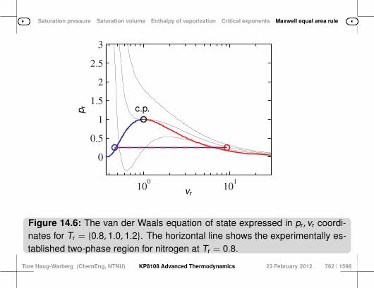
Saturation pressure Saturation volume Enthalpy of vaporization Critical exponents Maxwell equal area rule
100
101
0
0.5
1
1.5
2
2.5
3
c.p.
vr
p r
Figure 14.6: The van der Waals equation of state expressed in pr, vr coordi-nates for Tr = 0.8, 1.0, 1.2. The horizontal line shows the experimentally es-tablished two-phase region for nitrogen at Tr = 0.8.
Tore Haug-Warberg (ChemEng, NTNU) KP8108 Advanced Thermodynamics 23 February 2012 762 / 1598
Saturation pressure Saturation volume Enthalpy of vaporization Critical exponents Maxwell equal area rule
14 Simple . . .§ 111 § 110 § 112
The Maxwell equal area rule can be expressed as∫ Vv
V lıq(p − psat)(dV)T ,N = 0 and be plotted on a figureequivalent to 14.6, but with the ordinary volume andpressure along the axes. Show that this equation
actually holds for a one-component phase equilibrium.
Tore Haug-Warberg (ChemEng, NTNU) KP8108 Advanced Thermodynamics 23 February 2012 763 / 1598
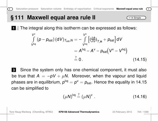
Saturation pressure Saturation volume Enthalpy of vaporization Critical exponents Maxwell equal area rule
14 Simple . . .§ 111 Maxwell equal area rule II
1 2 We immediately recognise −p as the partial derivative of Helmholtzenergy with respect to the volume along the chosen isotherm. The integral along this isotherm can be expressed as follows:
Vv∫
V lıq
(p − psat) (dV)Tsat,N = −Vv∫
V lıq
[(∂A∂V
)T ,n + psat
]dV
= A lıq − A v − psat
(Vv − V lıq
)
?= 0 . (14.15)
3 Since the system only has one chemical component, it must alsobe true that A = −pV + µN. Moreover, when the vapour and liquidphases are in equilibrium, p lıq = pv = psat. Hence the equality in 14.15can be simplified to
(µN)lıq ?= (µN)v . (14.16)
Tore Haug-Warberg (ChemEng, NTNU) KP8108 Advanced Thermodynamics 23 February 2012 764 / 1598

Saturation pressure Saturation volume Enthalpy of vaporization Critical exponents Maxwell equal area rule
14 Simple . . .§ 111 Maxwell equal area rule II (2)
4 The integration has been performed at constant temperature Tsat
and total composition N.5 Hence, as in 14.16, the mole number can be considered a constant
(common) factor for the vapour and liquid phases. It then follows that
µlıq = µv ,
which is identical to the phase equilibrium criterion for a one-componentsystem.
Tore Haug-Warberg (ChemEng, NTNU) KP8108 Advanced Thermodynamics 23 February 2012 765 / 1598

Saturation pressure Saturation volume Enthalpy of vaporization Critical exponents Maxwell equal area rule
14 Simple . . .§ 112 § 111 § 113
The necessary conditions for thermodynamic equilibriumin a closed system with only one chemical component,at a given temperature T , total volume V = Vv +V lıq
and total composition N = Nv + Nlıq, are
Aeq = minv,n
A(T , v,n) ,
ev = V ,
en = N .
Here e = [1 1], vT = [Vv V lıq] and nT = [Nv Nlıq]. Aswas mentioned at the start of this chapter, pv = p lıq
and µv = µlıq are necessary conditions for equilibrium.
Tore Haug-Warberg (ChemEng, NTNU) KP8108 Advanced Thermodynamics 23 February 2012 766 / 1598
Saturation pressure Saturation volume Enthalpy of vaporization Critical exponents Maxwell equal area rule
14 Simple . . .§ 112 § 111 § 113 (2)
Show that this is the case. Illustrate the energy surfaceusing a ρ,A diagram where ρr = v-1
r ∈ 〈0, 3〉.
Tore Haug-Warberg (ChemEng, NTNU) KP8108 Advanced Thermodynamics 23 February 2012 767 / 1598
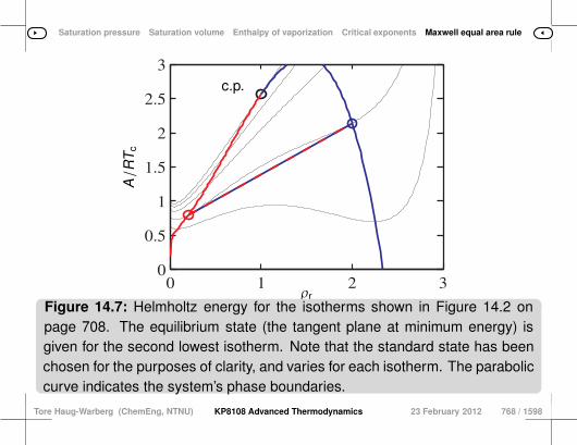
Saturation pressure Saturation volume Enthalpy of vaporization Critical exponents Maxwell equal area rule
0 1 2 30
0.5
1
1.5
2
2.5
3
ρr
A/R
Tc
c.p.
Figure 14.7: Helmholtz energy for the isotherms shown in Figure 14.2 onpage 708. The equilibrium state (the tangent plane at minimum energy) isgiven for the second lowest isotherm. Note that the standard state has beenchosen for the purposes of clarity, and varies for each isotherm. The paraboliccurve indicates the system’s phase boundaries.
Tore Haug-Warberg (ChemEng, NTNU) KP8108 Advanced Thermodynamics 23 February 2012 768 / 1598

Saturation pressure Saturation volume Enthalpy of vaporization Critical exponents Maxwell equal area rule
14 Simple . . .§ 112 Minimum of Helmholtz energy
1 A necessary — but not sufficient — condition for thermodynamicequilibrium is that (dA)T = 0 for variations in the extensive variablesVv,Nv and V lıq,Nlıq. Taking the total differential for both phases givesus
(dA)T = (dA)vT + (dA)
lıqT
= −pv dVv + µv dNv − p lıq dV lıq + µlıq dNlıq
= 0 .
2 The limits on the volume and mole number of the closed systemmean that dV lıq = − dVv and dNlıq = − dNv. Substituted into the differ-ential of A that gives us
(dA)T = −(pv − p lıq)dVv + (µv − µlıq)dNv = 0 .
Tore Haug-Warberg (ChemEng, NTNU) KP8108 Advanced Thermodynamics 23 February 2012 769 / 1598
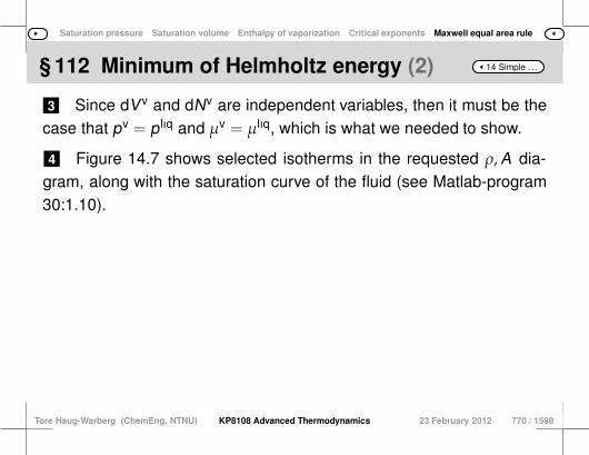
Saturation pressure Saturation volume Enthalpy of vaporization Critical exponents Maxwell equal area rule
14 Simple . . .§ 112 Minimum of Helmholtz energy (2)
3 Since dVv and dNv are independent variables, then it must be thecase that pv = p lıq and µv = µlıq, which is what we needed to show.
4 Figure 14.7 shows selected isotherms in the requested ρ,A dia-gram, along with the saturation curve of the fluid (see Matlab-program30:1.10).
Tore Haug-Warberg (ChemEng, NTNU) KP8108 Advanced Thermodynamics 23 February 2012 770 / 1598
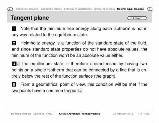
Saturation pressure Saturation volume Enthalpy of vaporization Critical exponents Maxwell equal area rule
14 Simple . . .Tangent plane
1 Note that the minimum free energy along each isotherm is not inany way related to the equilibrium state.
2 Helmholtz energy is a function of the standard state of the fluid,and since standard state properties do not have absolute values, theminimum of the function won’t be an absolute value either.
4 3 Admittedly we have found the minimum of the Helmholtz energyfunction, but we did that by distributing the total mass across two differ-ent phases. The equilibrium state is therefore characterised by having two
points on a single isotherm that can be connected by a line that is en-tirely below the rest of the function surface (the graph).
5 From a geometrical point of view, this condition will be met if thetwo points have a common tangent.6 It can be shown that the axis intercepts in the diagram are propor-
tional to p and µ respectively, which means that the tangent require-ment is also equivalent to pv = p lıq and µv = µlıq.7 This can be considered the result of a differential condition for equi-librium, whereas the Maxwell equal area rule is an integral formulationof the same condition.
Tore Haug-Warberg (ChemEng, NTNU) KP8108 Advanced Thermodynamics 23 February 2012 771 / 1598
Direct substitution Newton–Raphson iteration Chemical potential versus K -value Convergence properties
Part 15
Multicomponent Phase Equilibrium
see also Part-Contents
Tore Haug-Warberg (ChemEng, NTNU) KP8108 Advanced Thermodynamics 23 February 2012 772 / 1598
Direct substitution Newton–Raphson iteration Chemical potential versus K -value Convergence properties
Contents
1 Direct substitution
2 Newton–Raphson iteration
3 Chemical potential versus K -value
1 Equal fugacity models in both phases2 Equal activity models in both phases3 Mixed use of fugacity and activity models4 Mixed use of activity models in the phases
4 Convergence properties
Tore Haug-Warberg (ChemEng, NTNU) KP8108 Advanced Thermodynamics 23 February 2012 773 / 1598

Direct substitution Newton–Raphson iteration Chemical potential versus K -value Convergence properties
15 Multicomponent . . .Minimum energy
1 At thermodynamic equilibrium the system has reached a state ofminimum energy.
3 2 This far-reaching postulate is of tremendous importance for our un-derstanding of matter and energy, but it remains to discuss which of theenergy functions that are being minimised. In Chapter 16 on page 820 it is for example proved that Gibbs
energy of a closed system decreases (due to chemical reactions) tillthe minimum value Geq = minn G(T , p,n) is reached.
5 4 This is generally true when the temperature and pressure are con-stant. If the volume is kept constant and the pressure is varied the
Helmholtz energy will be minimised.
6 Chapter 14 on page 698 illustrates this for the case of a simplevapour–liquid equilibrium.7 The other energy functions U, H, etc. are minimised at constant
values of their respective canonical variables.
Tore Haug-Warberg (ChemEng, NTNU) KP8108 Advanced Thermodynamics 23 February 2012 774 / 1598
Direct substitution Newton–Raphson iteration Chemical potential versus K -value Convergence properties
15 Multicomponent . . .ω phases
1 In general we shall investigate a closed system consisting of π = α,
β, . . . , ψ, ω phases1 and a set of i = 1, 2, . . . , n components which arecommon to all the phases.
3 2 Reacting systems with (maybe) disjoint sets of the components ineach of the phases is taken up in Chapter Phase Reactions. For the special case of constant temperature and pressure
(dG)T ,p,n =∑ωπ=α
∑ni=1 µ
πi dNπ
i = 0 is a necessary condition for ther-modynamic equilibrium.
4 From the mass balance it follows that∑ωπ=α Nπ
i = Ni and even∑ωπ=α dNπ
i = 0 because the total moles Ni are constant.
Tore Haug-Warberg (ChemEng, NTNU) KP8108 Advanced Thermodynamics 23 February 2012 775 / 1598

Direct substitution Newton–Raphson iteration Chemical potential versus K -value Convergence properties
15 Multicomponent . . .ω phases (2)
6 5 The main concern of this chapter is a two-phase system where αand β may include vapour–liquid, liquid–liquid, solid–liquid and solid–solid equilibrium. The thermodynamic equilibrium criterion is then simplified to:
(dG)T ,p,n =n∑
i=1µαi dNα
i +n∑
i=1µβi dNβ
i = 0 ,
dNαi + dNβ
i = 0 .
Elimination of dNβi makes (dG)T ,p,n =
∑ni=1(µ
αi − µ
βi )dNα
i = 0.
7 In the vicinity of an equilibrium point all the dNαi are independent
quantities2 and the equilibrium relationship is equivalent to:
µαi = µβi , ∀i ∈ [1, n] . (15.1)
1 Phase α is usually the low temperature phase and β, . . . , ψ, ω are phases that becomestable at successively increasing temperatures.2 At equilibrium dNα
i are fluctuations beyond our control. These fluctuations are quiteinevitable from the laws of quantum mechanics and will be observed in every physicallyacceptable system. Thermodynamic equilibria are in other words dynamic, not static.
Tore Haug-Warberg (ChemEng, NTNU) KP8108 Advanced Thermodynamics 23 February 2012 776 / 1598

Direct substitution Newton–Raphson iteration Chemical potential versus K -value Convergence properties
15 Multicomponent . . .§ 113 § 112 § 114
Show that the necessary criteria for multiphase equilibriumat given total entropy S, total volume V and total
composition Ni for each component i, are Tα = T β =
. . . = Tω, pα = pβ = . . . = pω and µα = µβ = . . . = µω.It is assumed that all the components i ∈ [1, n] arepresent in all the phases α, β, . . . ω. Hint: start from
Ueq = mins,v,ni
U(s, v,n1, · · · ,nn) ,
es = S ,
ev = V ,
eni = Ni , ∀i ∈ [1, n] ,
Tore Haug-Warberg (ChemEng, NTNU) KP8108 Advanced Thermodynamics 23 February 2012 777 / 1598
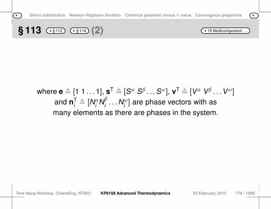
Direct substitution Newton–Raphson iteration Chemical potential versus K -value Convergence properties
15 Multicomponent . . .§ 113 § 112 § 114 (2)
where e = [1 1 . . .1], sT = [Sα Sβ . . .Sω], vT = [Vα Vβ . . .Vω]
and nTi = [Nα
i Nβi . . .N
ωi ] are phase vectors with as
many elements as there are phases in the system.
Tore Haug-Warberg (ChemEng, NTNU) KP8108 Advanced Thermodynamics 23 February 2012 778 / 1598
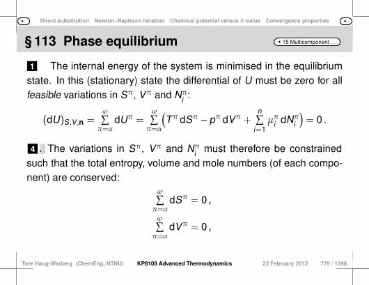
Direct substitution Newton–Raphson iteration Chemical potential versus K -value Convergence properties
15 Multicomponent . . .§ 113 Phase equilibrium
1 The internal energy of the system is minimised in the equilibriumstate. In this (stationary) state the differential of U must be zero for allfeasible variations in Sπ, Vπ and Nπ
i :
(dU)S,V ,n =ω∑π=α
dUπ =ω∑π=α
(Tπ dSπ − pπ dVπ +
n∑i=1µπi dNπ
i
)= 0 .
4 2 Note that U has no absolute minimum.3 Due to its extensive properties it will → ±∞ when the system size→∞. The variations in Sπ, Vπ and Nπ
i must therefore be constrainedsuch that the total entropy, volume and mole numbers (of each compo-nent) are conserved:
ω∑π=α
dSπ = 0 ,
ω∑π=α
dVπ = 0 ,
Tore Haug-Warberg (ChemEng, NTNU) KP8108 Advanced Thermodynamics 23 February 2012 779 / 1598

Direct substitution Newton–Raphson iteration Chemical potential versus K -value Convergence properties
15 Multicomponent . . .§ 113 Phase equilibrium (2)
ω∑π=α
dNπi = 0 , ∀i ∈ [1, n] .
6 5 From these n + 2 balance equations we can eliminate dSω, dVω
and dNωi for all the components i ∈ [1, n]. Substituted into the differential of U:
(dU)S,V ,n =ψ∑π=α
[(Tπ−Tω)dSπ− (pπ−pω)dVπ+
n∑i=1
(µπi −µωi )dNπ
i
]= 0 .
8 7 In the neighbourhood of an equilibrium point the quantitiesdSα , . . . , dSψ and dVα , . . . , dVψ and dN1
α , . . . , dSψn are truly indepen-
dent variables. If (dU)S,V ,n = 0 then it must be true that:
Tα = Tβ = · · · = Tψ = Tω ,
pα = pβ = · · · = pψ = pω ,
µα1 = µβ1 = · · · = µ
ψ1 = µω1 ,
...
µαn = µβn = · · · = µ
ψn = µωn .
Tore Haug-Warberg (ChemEng, NTNU) KP8108 Advanced Thermodynamics 23 February 2012 780 / 1598

Direct substitution Newton–Raphson iteration Chemical potential versus K -value Convergence properties
15 Multicomponent . . .§ 113 Phase equilibrium (3)
Tore Haug-Warberg (ChemEng, NTNU) KP8108 Advanced Thermodynamics 23 February 2012 781 / 1598

Direct substitution Newton–Raphson iteration Chemical potential versus K -value Convergence properties
15 Multicomponent . . .Gibbs’ phase rule
1 Despite the fact that temperature, pressure and chemical poten-tials are uniform at thermodynamic equilibrium we cannot specify thesevariables directly.
2 The Gibbs–Duhem’s equation
s dT − v dp + [n1 n2 · · · nn]dµ = 0 .
removes one degree of freedom per phase.
3 The number of independent intensive variables in a system istherefore F = dim(n) + 2 − dim(e), or in other words F = N + 2 − P,also known as the Gibbs phase rule for un-reacting systems.
Tore Haug-Warberg (ChemEng, NTNU) KP8108 Advanced Thermodynamics 23 February 2012 782 / 1598
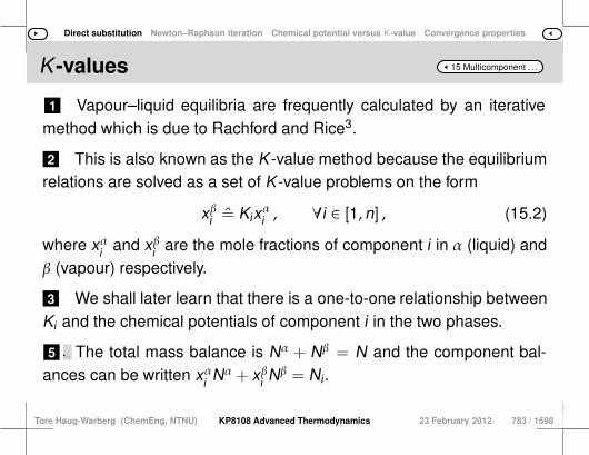
Direct substitution Newton–Raphson iteration Chemical potential versus K -value Convergence properties
15 Multicomponent . . .K -values
1 Vapour–liquid equilibria are frequently calculated by an iterativemethod which is due to Rachford and Rice3.
2 This is also known as the K -value method because the equilibriumrelations are solved as a set of K -value problems on the form
xβi = Kixαi , ∀i ∈ [1, n] , (15.2)
where xαi and xβi are the mole fractions of component i in α (liquid) andβ (vapour) respectively.
3 We shall later learn that there is a one-to-one relationship betweenKi and the chemical potentials of component i in the two phases.
5 4 This tells us that the K -value method can be applied even whenα and β are two arbitrary phases, but prior to the discussion of exoticphase equilibria we shall derive a calculation scheme (algorithm) forEq. 15.2. The total mass balance is Nα + Nβ = N and the component bal-
ances can be written xαi Nα + xβi Nβ = Ni.
Tore Haug-Warberg (ChemEng, NTNU) KP8108 Advanced Thermodynamics 23 February 2012 783 / 1598

Direct substitution Newton–Raphson iteration Chemical potential versus K -value Convergence properties
15 Multicomponent . . .K -values (2)
6 Elimination of Nβ produces xαi Nα + xβi (N − Nα) = Ni and a subse-quent substitution of xβi from Eq. 15.2 yields:
xαi = NiNα+Ki(N−Nα) =
zizα+Kizβ
. (15.3)
3 H. H. Rachford and J. D. Rice. Trans. Am. Inst. Min., Metall. Pet. Eng., 195:327–328,1952.
Tore Haug-Warberg (ChemEng, NTNU) KP8108 Advanced Thermodynamics 23 February 2012 784 / 1598

Direct substitution Newton–Raphson iteration Chemical potential versus K -value Convergence properties
15 Multicomponent . . .Rachford–Rice
1 The corresponding expression for xβi is
xβi = KiNiNα+Ki(N−Nα) =
Kizizα+Kizβ
, (15.4)
where zα = Nα/(Nα+Nβ) and zβ = Nβ/(Nα+Nβ) are the phase fractionsand zi = Ni/N is the total (feed) mole fraction of component i.
2 Note that the right hand sides of Eqs. 15.3 and 15.4 contain a singleunknown variable zα, or equivalently zβ = 1 − zα.
Tore Haug-Warberg (ChemEng, NTNU) KP8108 Advanced Thermodynamics 23 February 2012 785 / 1598
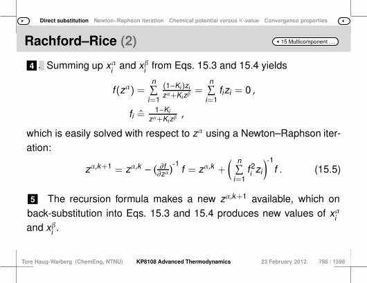
Direct substitution Newton–Raphson iteration Chemical potential versus K -value Convergence properties
15 Multicomponent . . .Rachford–Rice (2)
4 3 Definition-wise∑n
i xi = 1 in both phases and it is possible tosolve for zα from Eq. 15.3 or 15.4, but practical experience provesthat the algorithm is more stable when the symmetric condition f(zα) =∑n
i=1(xαi − xβi ) = 0 is being used. Summing up xαi and xβi from Eqs. 15.3 and 15.4 yields
f(zα) =n∑
i=1
(1−Ki)zi
zα+Kizβ=
n∑i=1
fizi = 0 ,
fi =1−Ki
zα+Kizβ,
which is easily solved with respect to zα using a Newton–Raphson iter-ation:
zα,k+1 = zα,k − ( ∂f∂zα
)-1f = zα,k +
( n∑i=1
f2i zi
)-1f . (15.5)
5 The recursion formula makes a new zα,k+1 available, which onback-substitution into Eqs. 15.3 and 15.4 produces new values of xαiand xβi .
Tore Haug-Warberg (ChemEng, NTNU) KP8108 Advanced Thermodynamics 23 February 2012 786 / 1598

Direct substitution Newton–Raphson iteration Chemical potential versus K -value Convergence properties
15 Multicomponent . . .Rachford–Rice (3)
6 These updates (hopefully) improve the Ki-values, and subsequentiterates in Eq. 15.5 converge finally to the equilibrium state.
Tore Haug-Warberg (ChemEng, NTNU) KP8108 Advanced Thermodynamics 23 February 2012 787 / 1598
Direct substitution Newton–Raphson iteration Chemical potential versus K -value Convergence properties
15 Multicomponent . . .§ 114 § 113 § 115
Computerise the function [xα, xβ, zα] = TpKvalue(n, k)using Eq. 15.5 as your reference algorithm.
Tore Haug-Warberg (ChemEng, NTNU) KP8108 Advanced Thermodynamics 23 February 2012 788 / 1598
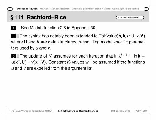
Direct substitution Newton–Raphson iteration Chemical potential versus K -value Convergence properties
15 Multicomponent . . .§ 114 Rachford–Rice
1 See Matlab function 2.6 in Appendix 30.
3 2 Note that the function interface is more elaborate than has beenasked for in the text. The syntax has notably been extended to TpKvalue(n, k, u,U, v,V)
where U and V are data structures transmitting model specific parame-ters used by u and v.
5 4 This makes it possible to iterate on non-ideal equilibrium states bysupplying two fugacity (activity) coefficient models u and v. The update of Ki assumes for each iteration that ln kk+1 = ln k +
u(xα,U) − v(xβ,V). Constant Ki values will be assumed if the functionsu and v are expelled from the argument list.
Tore Haug-Warberg (ChemEng, NTNU) KP8108 Advanced Thermodynamics 23 February 2012 789 / 1598
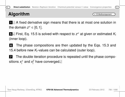
Direct substitution Newton–Raphson iteration Chemical potential versus K -value Convergence properties
15 Multicomponent . . .Algorithm
1 2 Note that ∂f/∂zα < 0 in Eq. 15.5 except for the degenerated caseKi = 1∀i ∈ [1, n] then ∂f/∂zα = 0. A fixed derivative sign means that there is at most one solution in
the domain zα ∈ [0, 1].
5 3 Similar to the Newton–Rapshon method, which is derived in Sec-tion 15.2, the number of floating point operations in the update of xα isproportional to n, i.e. the computation time increases linearly with thenumber of components in the system.4 These are the strengths of the K -value method, but it has also an
inherit weakness in that non-ideal equilibria must be solved by nestediteration. First, Eq. 15.5 is solved with respect to zα at given or estimated Ki
(inner loop).
6 The phase compositions are then updated by the Eqs. 15.3 and15.4 before new Ki-values can be calculated (outer loop).
7 The double iteration procedure is repeated until the phase compo-sitions xαi and xβi have converged.8 The Newton–Raphson method in Section 15.2 is without this flaw
because ∆µi (equivalent to Ki) is updated in every iteration avoiding theouter loopa.
a Also applies to the K -value problem if disregarding the monotonic form of f(zα).
Tore Haug-Warberg (ChemEng, NTNU) KP8108 Advanced Thermodynamics 23 February 2012 790 / 1598

Direct substitution Newton–Raphson iteration Chemical potential versus K -value Convergence properties
15 Multicomponent . . .Newton–Raphson
1 Contrary to the K -value method of Rachford–Rice, the Newton4–Raphson5s method fulfills the mass balance in every iteration.
2 This requires a feasible starting point where nα+nβ = n is fulfilled.
3 The Newton–Raphson iteration of Eq. 15.1 is then,
µαi +n∑
j=1
(∂µαi∂Nα
j
)T ,p,Nl,j
∆Nαj = µβi +
n∑j=1
(∂µβi∂Nβ
j
)T ,p,Nl,j
∆Nβj ,
−∆Nβj = ∆Nα
j ,
or on matrix form:
µα + Gα∆nα = µβ + Gβ∆nβ ,
−∆nβ = ∆nα .
4 Sir Isaac Newton, 1642–1727 by the Julian calendar. English physicist and mathe-matician.5 .Tore Haug-Warberg (ChemEng, NTNU) KP8108 Advanced Thermodynamics 23 February 2012 791 / 1598

Direct substitution Newton–Raphson iteration Chemical potential versus K -value Convergence properties
15 Multicomponent . . .Algorithm
1 The matrix G = (∂2G/∂Ni∂Nj)T ,p is the Hessian6 of Gibbs energyand ∆n = nk+1 −nk is the composition difference between two (subse-quent) iterations k + 1 and k .
2 The Newton–Raphson equations can be combined into
(Gα + Gβ)∆nα = −(µα − µβ) ,
or even better: ∆nα = −H-1∆µ where H = Gα + Gβ and ∆µ = µα − µβ.4 3 It must be realised, however, that the algorithm has to be guided. In particular the mole number updates must be checked for
nα,k+1 = nα,k +∆nα > 0 and nβ,k+1 = nβ,k −∆nα > 0.
Tore Haug-Warberg (ChemEng, NTNU) KP8108 Advanced Thermodynamics 23 February 2012 792 / 1598
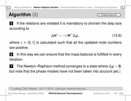
Direct substitution Newton–Raphson iteration Chemical potential versus K -value Convergence properties
15 Multicomponent . . .Algorithm (2)
5 If the relations are violated it is mandatory to shorten the step sizeaccording to
∆nα = −τH-1∆µ , (15.6)
where τ ∈ 〈0, 1] is calculated such that all the updated mole numbersare positive.
6 In this way we can ensure that the mass balance is fulfilled in everyiteration.
7 The Newton–Raphson method converges to a state where ∆µ = 0,but note that the phase models have not been taken into account yet.8 It must therefore be anticipated that ∆µ is calculated from an equa-
tion of state, or an activity model, that describes the system with suffi-cient accuracy.
6 Ludwig Otto Hesse, 1811–1874. German mathematician.
Tore Haug-Warberg (ChemEng, NTNU) KP8108 Advanced Thermodynamics 23 February 2012 793 / 1598
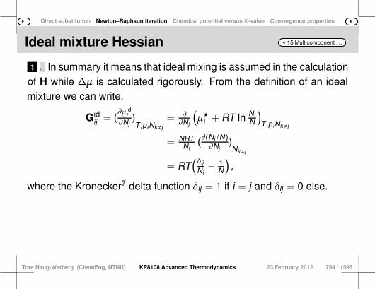
Direct substitution Newton–Raphson iteration Chemical potential versus K -value Convergence properties
15 Multicomponent . . .Ideal mixture Hessian
1 2 The calculation of H may be approximated by the Hessian of anideal mixture.3 The convergence properties will deteriorate close to the solution
compared to the rigorous implementation of H = Gα + Gβ, but the sim-plicity of the model makes it interesting in its own right. In summary it means that ideal mixing is assumed in the calculation
of H while ∆µ is calculated rigorously. From the definition of an idealmixture we can write,
Gıdij =
(∂µıdi
∂Nj
)T ,p,Nk,j
= ∂∂Nj
(µ⋆i + RT ln Ni
N
)T ,p,Nk,j
= NRTNi
(∂(Ni/N)∂Nj
)Nk,j
= RT( δij
Ni− 1
N
),
where the Kronecker7 delta function δij = 1 if i = j and δij = 0 else.
Tore Haug-Warberg (ChemEng, NTNU) KP8108 Advanced Thermodynamics 23 February 2012 794 / 1598
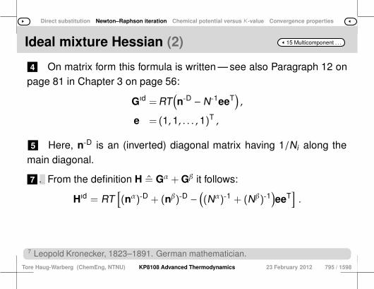
Direct substitution Newton–Raphson iteration Chemical potential versus K -value Convergence properties
15 Multicomponent . . .Ideal mixture Hessian (2)
4 On matrix form this formula is written — see also Paragraph 12 onpage 81 in Chapter 3 on page 56:
Gıd =RT(n-D − N-1eeT
),
e =(1, 1, . . . , 1)T ,
5 Here, n-D is an (inverted) diagonal matrix having 1/Ni along themain diagonal.
7 6 The simple structure of this matrix makes it possible to calculateH-1 with an analytical formula as shown below. From the definition H = Gα + Gβ it follows:
Hıd = RT[(nα)-D + (nβ)-D −
((Nα)-1 + (Nβ)-1
)eeT
].
7 Leopold Kronecker, 1823–1891. German mathematician.
Tore Haug-Warberg (ChemEng, NTNU) KP8108 Advanced Thermodynamics 23 February 2012 795 / 1598

Direct substitution Newton–Raphson iteration Chemical potential versus K -value Convergence properties
15 Multicomponent . . .Sherman–Morrison
1 The matrix (nα)-D+(nβ)-D has diagonal elements (Nαi )
-1+(Nβi )
-1 =
Ni/(Nαi Nβ
i ) and the factor (Nα)-1 + (Nβ)-1 can be rewritten to (Nα +
Nβ)/(NαNβ).
2 This makes the following factorisation of Hıd possible:
Hıd = RT Nα+Nβ
NαNβ
[diag
(NαNβ
Nαi Nβ
i
Ni
(Nα+Nβ)
)− eeT
],
or,
Nα+Nβ
RT Hıd = 1zαzβ (D
-1 − eeT) ,
D-1 = diag( zi
xαi xβi
), (15.7)
where zα and zβ are phase fractions, xαi and
3 As usual xβi are component mole fractions, and zi is the feed molefraction of component i.
Tore Haug-Warberg (ChemEng, NTNU) KP8108 Advanced Thermodynamics 23 February 2012 796 / 1598
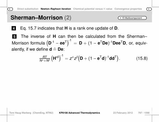
Direct substitution Newton–Raphson iteration Chemical potential versus K -value Convergence properties
15 Multicomponent . . .Sherman–Morrison (2)
4 Eq. 15.7 indicates that H is a rank one update of D.
5 The inverse of H can then be calculated from the Sherman–
Morrison formula(D-1 − eeT
)-1= D + (1 − eTDe)-1DeeTD, or, equiv-
alently, if we define d = De:
RTNα+Nβ
(Hıd
)-1= zαzβ
(D + (1 − eTd)-1ddT
). (15.8)
Tore Haug-Warberg (ChemEng, NTNU) KP8108 Advanced Thermodynamics 23 February 2012 797 / 1598
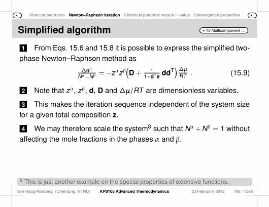
Direct substitution Newton–Raphson iteration Chemical potential versus K -value Convergence properties
15 Multicomponent . . .Simplified algorithm
1 From Eqs. 15.6 and 15.8 it is possible to express the simplified two-phase Newton–Raphson method as
∆nα
Nα+Nβ = −zαzβ(D + 1
1−dTeddT
)∆µ
RT . (15.9)
2 Note that zα, zβ, d, D and ∆µ/RT are dimensionless variables.
3 This makes the iteration sequence independent of the system sizefor a given total composition z.
4 We may therefore scale the system8 such that Nα+Nβ = 1 withoutaffecting the mole fractions in the phases α and β.
8 This is just another example on the special properties of extensive functions.
Tore Haug-Warberg (ChemEng, NTNU) KP8108 Advanced Thermodynamics 23 February 2012 798 / 1598
Direct substitution Newton–Raphson iteration Chemical potential versus K -value Convergence properties
15 Multicomponent . . .§ 115 § 114 § 116
The Sherman–Morrison formula is widely applicableand not at all limited to thermodynamic problems.
Verify the formula by proving that H-1H = I. Attemptto find a more general formula valid for (A − uvT)-1.
Tore Haug-Warberg (ChemEng, NTNU) KP8108 Advanced Thermodynamics 23 February 2012 799 / 1598
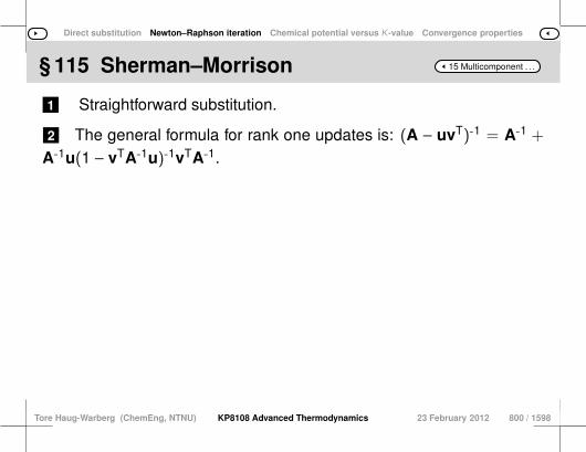
Direct substitution Newton–Raphson iteration Chemical potential versus K -value Convergence properties
15 Multicomponent . . .§ 115 Sherman–Morrison
1 Straightforward substitution.
2 The general formula for rank one updates is: (A − uvT)-1 = A-1 +
A-1u(1 − vTA-1u)-1vTA-1.
Tore Haug-Warberg (ChemEng, NTNU) KP8108 Advanced Thermodynamics 23 February 2012 800 / 1598
Direct substitution Newton–Raphson iteration Chemical potential versus K -value Convergence properties
15 Multicomponent . . .§ 116 § 115 § 117
Computerise the function [xα, xβ, zα] = TpNewton(n, k)using Eq. 15.9 as your reference algorithm.
Tore Haug-Warberg (ChemEng, NTNU) KP8108 Advanced Thermodynamics 23 February 2012 801 / 1598

Direct substitution Newton–Raphson iteration Chemical potential versus K -value Convergence properties
15 Multicomponent . . .§ 116 Newton–Raphson iteration
1 See Matlab function 2.7 in Appendix 30.
3 2 Note that the function interface is more elaborate than has beenasked for in the text. The syntax has notably been extended to TpNewton(n, k, u,U, v,V)
where U and V are data structures transmitting model specific parame-ters used by u and v.
4 This makes it possible to iterate on non-ideal equilibrium states bysupplying two fugacity (activity) coefficient models u and v.5 The update of ∆µ assumes that for each iteration ∆µ = ∆µıd +
∆µr,p where ∆µıd = ln k + ln xα − ln xβ and ∆µr,p = u(xα,U) − v(xβ,V).6 Constant ∆µr,p = 0 will be assumed if the functions u and v are
expelled from the argument list.
Tore Haug-Warberg (ChemEng, NTNU) KP8108 Advanced Thermodynamics 23 February 2012 802 / 1598
Direct substitution Newton–Raphson iteration Chemical potential versus K -value Convergence properties
15 Multicomponent . . .Ki versus µi Computation time1 It should be mentioned that the number of floating point operations
in the update is proportional to n.
2 Hence, the computation time increases linearly with the number ofcomponents in the mixture.
3 However, if we had not spent time on the Sherman–Morrison for-mula, but rather used numerical inversion of H in each iteration, thecomputation time would be proportional to n3.
803 / 1598
1 The Rachford–Rice procedure spends time on calculating K -valueswhile the Newton–Raphson method deals directly with chemical poten-tials.
2 However, because the two methods aim at solving the same prob-lem there must be a rational connection between them.
3 The purpose of this section is to show that (and how) Eq. 15.1 onpage 750 can be used to derive some useful relations between Ki and∆µi.
Tore Haug-Warberg (ChemEng, NTNU) KP8108 Advanced Thermodynamics 23 February 2012 804 / 1598

Direct substitution Newton–Raphson iteration Chemical potential versus K -value Convergence properties
15 Multicomponent . . .Fugacity / fugacity
1 For fluid p(V ,T) equations of state µi (T , p) is defined as thechemical potential of a pure ideal gas at the temperature T and pres-sure p.
2 The same standard state applies to both of the phases and fromµαi = µβi it is conventionally written
µi + RT ln(ϕαi xαi p
p
)= µi + RT ln
(ϕβi xβi pp
),
where the left side stands for µαi and the right side stands for µβi .
Tore Haug-Warberg (ChemEng, NTNU) KP8108 Advanced Thermodynamics 23 February 2012 805 / 1598

Direct substitution Newton–Raphson iteration Chemical potential versus K -value Convergence properties
15 Multicomponent . . .Fugacity / fugacity (2)
3 The quantity ∆µi/RT which appears in Eq. 15.9 is then
∆µiRT =
µαi −µβi
RT = ln(Keos
i xαixβi
), (15.10)
where K eosi is defined as the ratio between the fugacity coefficients ϕαi
and ϕβi :
K eosi =
ϕαiϕβi. (15.11)
4 In the context of being an equilibrium constant the K -value is there-fore quite misleading. Ki(T , p, xα, xβ) is in fact a non-linear function intemperature, pressure and the compositions of both phases.
Tore Haug-Warberg (ChemEng, NTNU) KP8108 Advanced Thermodynamics 23 February 2012 806 / 1598
Direct substitution Newton–Raphson iteration Chemical potential versus K -value Convergence properties
15 Multicomponent . . .§ 117 § 116 § 118
Find experimental data for a typical hydrocarbon vapour–liquid system and see how close the RK equationof state matches the measurements. Calculate the
phase diagram using TpKvalue or TpNewton.
Tore Haug-Warberg (ChemEng, NTNU) KP8108 Advanced Thermodynamics 23 February 2012 807 / 1598

Direct substitution Newton–Raphson iteration Chemical potential versus K -value Convergence properties
15 Multicomponent . . .§ 117 Natural gas
1 The phase diagram of a typical, albeit synthetic, natural gas9 isillustrated in Figure 15.1 on the following page.
2 The calculations are shown in Matlab program 30:1.22.
3 The plot is given a high colour density where the liquid and vapourphases coexist in approximately equal amounts, and a light colour nearthe single-phase region (vapour or liquid).4 The dense ridge running along the left edge of the diagram com-
bined with the shallow basin to the right is typical for methane-rich nat-ural gases.5 The bubble point is dominated by the large methane content while
the dew point is determined by the trace components comprising the“heavy tail” of the gas.6 The Newton–Raphson method does an excellent job in this casea,7 but note that the dew-point calculations are sensitive to the start
estimate.8 Increasing the liquid composition of the medium components by
less than one tenth of a mole fraction causes the rightmost part of thephase boundary to be left out.9 The K -value method has even larger problems in this part of the
diagram, and needs some type of guidance which is not implementedhere.
a Far better than anticipated. In fact, it does a better job than for a rigorous imple-mentation of the Hessian. The reason for this somewhat strange behaviour is that theeigenvalues of the simplified Hessian are strictly positive while the eigenvalues of therigorous Hessian change sign wherever thermodynamic instability occurs, see Chap-ter 21. This is known to cause numerical problems in Newton–Raphson methods.
9 Mario H. Gonzalez and Anthony L. Lee. J. Chem. Eng. Data, 13(2):172–176, April1968.
Tore Haug-Warberg (ChemEng, NTNU) KP8108 Advanced Thermodynamics 23 February 2012 808 / 1598
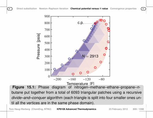
Direct substitution Newton–Raphson iteration Chemical potential versus K -value Convergence properties
−200 −160 −120 −800
100
200
300
400
500
600
700
800
900
Temperature [F]
Pre
ssur
e[p
sia]
c.p.
N = 2913
Figure 15.1: Phase diagram of nitrogen–methane–ethane–propane–n-butane put together from a total of 6093 triangular patches using a recursivedivide–and–conquer algorithm (each triangle is split into four smaller ones un-til all the vertices are in the same phase domain).
Tore Haug-Warberg (ChemEng, NTNU) KP8108 Advanced Thermodynamics 23 February 2012 809 / 1598

Direct substitution Newton–Raphson iteration Chemical potential versus K -value Convergence properties
15 Multicomponent . . .§ 118 § 117 § 119Physical chemistry1 In the ages before the modern computer era it was mandatory to
make physical simplifications before any numerical calculation was at-tempted.
2 One of these simplifications is known as the Lewis mixing rule.
3 Under certain circumstances the fugacity coefficient ϕi will be al-most independent of the mixture composition.
4 This is always true for an ideal gas mixture and it is valid to ahigh degree of approximation for real gases at low pressures or hightemperatures.
5 The approximation also holds at high pressures if ∆Vex ≈ 0 in theentire pressure and composition region.
6 In the case of ϕi(T , p, x) ≈ ϕ⋆i (T , p) then Ki will be constant inEq. 15.11 (at a given temperature and pressure).
7 The K -value method is then superior to the Newton–Raphson iter-ation because it solves the entire equilibrium problem in R1 and not inRn.
810 / 1598
Show that the Lewis mixing rule is exact if Amagat10slaw Vex = 0 is valid over the entire composition and
pressure [0, p] range.
10 Émile Hilaire Amagat, 1841–1915. French chemist.
Tore Haug-Warberg (ChemEng, NTNU) KP8108 Advanced Thermodynamics 23 February 2012 811 / 1598
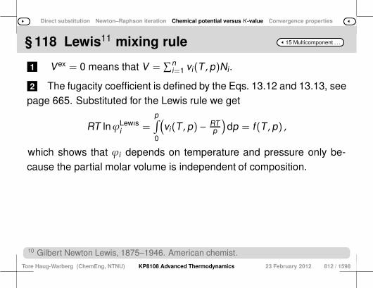
Direct substitution Newton–Raphson iteration Chemical potential versus K -value Convergence properties
15 Multicomponent . . .§ 118 Lewis11 mixing rule
1 Vex = 0 means that V =∑n
i=1 vi(T , p)Ni.
2 The fugacity coefficient is defined by the Eqs. 13.12 and 13.13, seepage 665. Substituted for the Lewis rule we get
RT lnϕLewısi =
p∫
0
(vi(T , p) − RT
p
)dp = f(T , p) ,
which shows that ϕi depends on temperature and pressure only be-cause the partial molar volume is independent of composition.
10 Gilbert Newton Lewis, 1875–1946. American chemist.
Tore Haug-Warberg (ChemEng, NTNU) KP8108 Advanced Thermodynamics 23 February 2012 812 / 1598

Direct substitution Newton–Raphson iteration Chemical potential versus K -value Convergence properties
15 Multicomponent . . .Activity / activity
1 In Eq. 15.11 it is common that α is the liquid phase and β the vapourphase, but this is just one out of many possibilities.
2 We could alternatively assume that α and β are two near-criticalfluids being something in between a vapour and a liquid, or two well-defined liquid phases.
7 3 There are also examples on supercritical gas–gas equilibria in theliterature.4 In a thermodynamic sense there is no fundamental difference be-
tween a vapour phase and a liquid phasea,5 but it is easy to decide whether the phases are of the same type by
looking at the pure component states in the system.6 If the chemical potentials of the pure components are the same in
both phases, at the temperature and pressure of the system, it can beconcluded that the phases are of the same nature.
a It is intuitive that the density of the vapour phase has to be lower than the densityof the liquid phase, but this is wrong. At high pressures the system H2–He will in factinvert because the vapour phase is dominated by He which has a higher molecularweight than H2. If this is the case it is no longer necessary to integrate all the way
from the ideal gas in Eq. 15.11 but rather use the pure componentproperties as a reference.
8 In practise this means that the fugacity coefficients can be replacedby activity coefficients:
K eosi =
ϕαiϕβi
=γαiγβi
ϕα,⋆iϕβ,⋆i
.
Tore Haug-Warberg (ChemEng, NTNU) KP8108 Advanced Thermodynamics 23 February 2012 813 / 1598
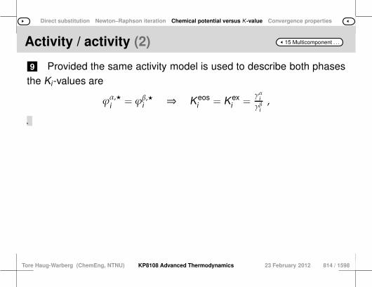
Direct substitution Newton–Raphson iteration Chemical potential versus K -value Convergence properties
15 Multicomponent . . .Activity / activity (2)
9 Provided the same activity model is used to describe both phasesthe Ki-values are
ϕα,⋆i = ϕβ,⋆i ⇒ K eosi = K ex
i =γαiγβi,
10 because the pure component reference ϕ⋆i is the same in bothphases.
Tore Haug-Warberg (ChemEng, NTNU) KP8108 Advanced Thermodynamics 23 February 2012 814 / 1598

Direct substitution Newton–Raphson iteration Chemical potential versus K -value Convergence properties
15 Multicomponent . . .§ 119 § 118 § 120
Find experimental data for a ternary liquid–liquid systemwith known NRTL, van Laar or Margules model parameters.
Select a system which has a fairly large solubility regionand a critical end-point inside the ternary region. Use
TpNewton to calculate the phase diagram.
Tore Haug-Warberg (ChemEng, NTNU) KP8108 Advanced Thermodynamics 23 February 2012 815 / 1598
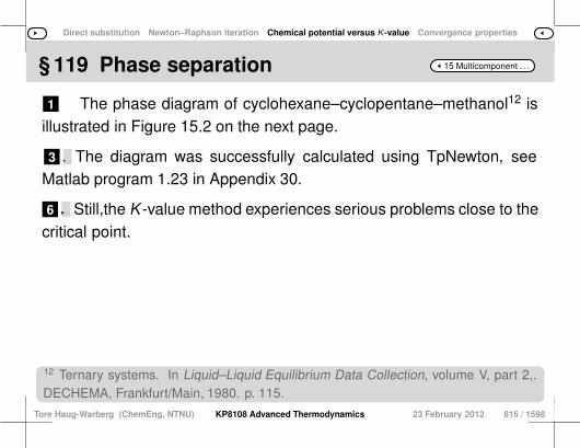
Direct substitution Newton–Raphson iteration Chemical potential versus K -value Convergence properties
15 Multicomponent . . .§ 119 Phase separation
1 The phase diagram of cyclohexane–cyclopentane–methanol12 isillustrated in Figure 15.2 on the next page.
3 2 It is a classic liquid–liquid diagram — quite symmetric and with acritical end-point inside the triangle. The diagram was successfully calculated using TpNewton, see
Matlab program 1.23 in Appendix 30.
6 4 In this case the measurements were used as start values and thecalculations converged without difficulty even in the vicinity of the criticalpoint of the mixture.5 The agreement between the measured and the calculated values
is otherwise extremely good. Still,the K -value method experiences serious problems close to thecritical point.
12 Ternary systems. In Liquid–Liquid Equilibrium Data Collection, volume V, part 2,.DECHEMA, Frankfurt/Main, 1980. p. 115.
Tore Haug-Warberg (ChemEng, NTNU) KP8108 Advanced Thermodynamics 23 February 2012 816 / 1598

Direct substitution Newton–Raphson iteration Chemical potential versus K -value Convergence properties
0 0.2 0.4 0.6 0.8 1
c.p.
Mole fraction of methanol
Mol
efra
ctio
nof
cycl
open
tane
Figure 15.2: Phase diagram of cyclohexane–cyclopentane–methanol at298.15 K and 760 mmHg. The iterations are started at interpolated pointsin the diagram (ensure safe convergence).
Tore Haug-Warberg (ChemEng, NTNU) KP8108 Advanced Thermodynamics 23 February 2012 817 / 1598
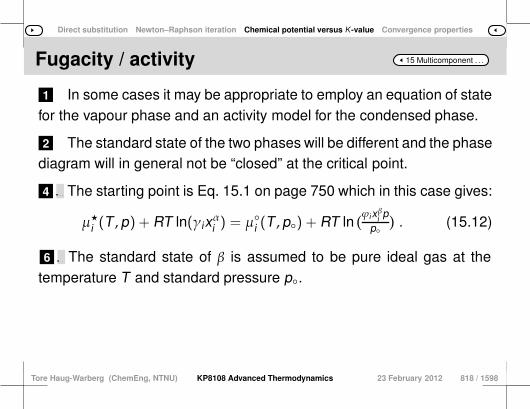
Direct substitution Newton–Raphson iteration Chemical potential versus K -value Convergence properties
15 Multicomponent . . .Fugacity / activity
1 In some cases it may be appropriate to employ an equation of statefor the vapour phase and an activity model for the condensed phase.
2 The standard state of the two phases will be different and the phasediagram will in general not be “closed” at the critical point.
4 3 On the other hand, hybrid models have greater flexibility and arefavourable in the modelling of complex liquids and crystal phases. The starting point is Eq. 15.1 on page 750 which in this case gives:
µ⋆i (T , p) + RT ln(γixαi ) = µi (T , p) + RT ln(ϕixβi p
p
). (15.12)
6 5 The left hand side denotes µαi and the right hand side µβi . The standard state of β is assumed to be pure ideal gas at thetemperature T and standard pressure p.
Tore Haug-Warberg (ChemEng, NTNU) KP8108 Advanced Thermodynamics 23 February 2012 818 / 1598

Direct substitution Newton–Raphson iteration Chemical potential versus K -value Convergence properties
15 Multicomponent . . .Fugacity / activity (2)
7 The reference state of phase α is in principle a function of temper-ature, pressure and composition, but in most cases a pure componentreference is used where limγi = 1.0 as p → psat
i , i.e. the referencepressure is set equal to the saturation pressure of component i:
µ⋆i (T , psati ) = µi + RT ln
(ϕsati psat
ip
). (15.13)
Tore Haug-Warberg (ChemEng, NTNU) KP8108 Advanced Thermodynamics 23 February 2012 819 / 1598
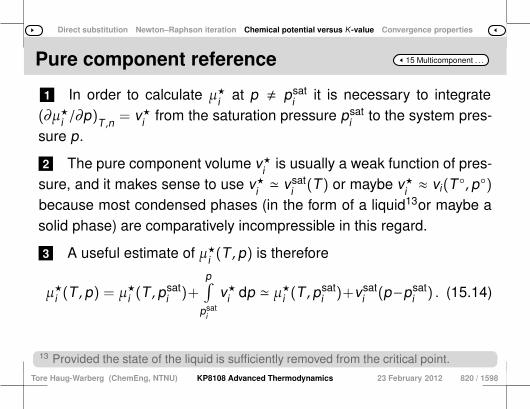
Direct substitution Newton–Raphson iteration Chemical potential versus K -value Convergence properties
15 Multicomponent . . .Pure component reference
1 In order to calculate µ⋆i at p , psati it is necessary to integrate
(∂µ⋆i /∂p)T ,n
= v⋆i from the saturation pressure psati to the system pres-
sure p.
2 The pure component volume v⋆i is usually a weak function of pres-sure, and it makes sense to use v⋆i ≃ vsat
i (T) or maybe v⋆i ≈ vi(T , p)because most condensed phases (in the form of a liquid13or maybe asolid phase) are comparatively incompressible in this regard.
3 A useful estimate of µ⋆i (T , p) is therefore
µ⋆i (T , p) = µ⋆i (T , psati )+
p∫
psati
v⋆i dp ≃ µ⋆i (T , psati )+vsat
i (p−psati ) . (15.14)
13 Provided the state of the liquid is sufficiently removed from the critical point.
Tore Haug-Warberg (ChemEng, NTNU) KP8108 Advanced Thermodynamics 23 February 2012 820 / 1598

Direct substitution Newton–Raphson iteration Chemical potential versus K -value Convergence properties
15 Multicomponent . . .Chemical potential
1 which is substituted into Eq. 15.13 and finally combined with theequilibrium relation in Eq. 15.12. The result is:
µi + RT ln(ϕsat
i psati γixαip
)+ vsat
i (p − psati ) ≈ µi + RT ln
(ϕixβi pp
).
2 ∆µi/RT from the Newton–Raphson algorithm in Eq. 15.9 may nowbe written on the same form as in Eq. 15.10 provided Ki is calculatedas
K vlei =
ϕsati psat
i γi
ϕipexp
(vsati (p−psat
i )
RT), (15.15)
The exponential term is known as the Poynting14 factor of Ki.3 This factor is often neglected at low pressures, but only if Ki 1.4 If this is not true the Poynting-factor may dominate Ki down to 5 −
10 bar.
14 John Henry Poynting, 1852–1914. English physicist.
Tore Haug-Warberg (ChemEng, NTNU) KP8108 Advanced Thermodynamics 23 February 2012 821 / 1598

Direct substitution Newton–Raphson iteration Chemical potential versus K -value Convergence properties
15 Multicomponent . . .Raoult15s law
1 For an approximately pure liquid component i it is reasonable to setϕi = ϕsat
i , γi = 1 and p = psati .
2 The mixture is by definition ideal and Ki appears to be a simplefunction of temperature and pressure:
K Raoulti = lim
xi→1K vle
i =psat
ip
14 François-Marie Raoult, 1830–1901. French chemist.
Tore Haug-Warberg (ChemEng, NTNU) KP8108 Advanced Thermodynamics 23 February 2012 822 / 1598
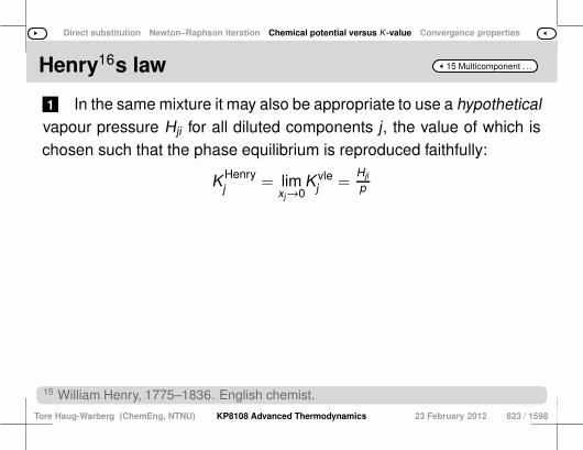
Direct substitution Newton–Raphson iteration Chemical potential versus K -value Convergence properties
15 Multicomponent . . .Henry16s law
1 In the same mixture it may also be appropriate to use a hypotheticalvapour pressure Hji for all diluted components j, the value of which ischosen such that the phase equilibrium is reproduced faithfully:
K Henryj = lim
xj→0K vle
j =Hji
p
15 William Henry, 1775–1836. English chemist.
Tore Haug-Warberg (ChemEng, NTNU) KP8108 Advanced Thermodynamics 23 February 2012 823 / 1598

Direct substitution Newton–Raphson iteration Chemical potential versus K -value Convergence properties
15 Multicomponent . . .§ 120 § 119 § 121
Find experimental data for a close to ideal binaryvapour–liquid system with known NRTL, Wilson, van
Laar or Margules model parameters. Use TpKvalue orTpNewton to calculate the phase diagram. Comment
on the practical applicability of Raoult’s law versusthe accuracy of pure component data.
Tore Haug-Warberg (ChemEng, NTNU) KP8108 Advanced Thermodynamics 23 February 2012 824 / 1598

Direct substitution Newton–Raphson iteration Chemical potential versus K -value Convergence properties
15 Multicomponent . . .§ 120 Ideal mixture
1 The phase diagram of hexane–toluene17 is illustrated in Fig-ure 15.3 on the next page.
2 The calculations make use of the Matlab program 1.24 in Ap-pendix 30.
4 3 The system is almost ideal, but there are nevertheless some no-table deviations between the experimental and the calculated values. Correcting for non-ideality makes some improvement (compare σ1
and σ2 in the left subfigure), but the largest error is actually hidden inthe vapour pressure of toluene.
5 By increasing the vapour pressure 2% the agreement is improvedeven further (compare σ3 and σ4 in the right subfigure), while Raoult’slaw still shows a significant deviation from the measurements.6 This shows that Raoult’s law is of limited value even for nearly ideal
systems.7 In fact, the pure component parameters are maybe more importantfor the mixture properties than the phase model itself.
17 Aliphatic hydrocarbons: C4–C6. In Vapor–Liquid Equilibrium Data Collection, volumeI, part 6a,. DECHEMA, Frankfurt/Main, 1980. p. 593.
Tore Haug-Warberg (ChemEng, NTNU) KP8108 Advanced Thermodynamics 23 February 2012 825 / 1598

Direct substitution Newton–Raphson iteration Chemical potential versus K -value Convergence properties
0 0.5 160
80
100
120
0 0.5 160
80
100
120
Mole fraction of hexaneMole fraction of hexane
Tem
pera
ture
[C]
Antoine vapour pressure Corrected vapour pressure
σ1 = 0.356σ2 = 0.157
σ3 = 0.265σ4 = 0.095
Figure 15.3: Phase diagram of hexane–toluene at 760 mmHg. Calculatedcurves show Raoult’s law (stipled) and van Laar activity (solid). The rightsubfigure shows the effect of increasing the vapour pressure of toluene by2%. The sum-of-squares are denoted σ1, σ2, σ3 and σ4.
Tore Haug-Warberg (ChemEng, NTNU) KP8108 Advanced Thermodynamics 23 February 2012 826 / 1598

Direct substitution Newton–Raphson iteration Chemical potential versus K -value Convergence properties
15 Multicomponent . . .Acitivity / activity
1 When α and β are condensed phases it is often appropriate toneglect the influence of pressure on the system properties.
2 This is quite typical for metallurgical melts and refractory systemswhere the process conditions are close to atmospheric. 3 In general, pressure explicit equations of state are not conceivable
for these systems and activity models are often used for both phases:
µα,⋆i (T ) + RT ln(γαi xαi ) = µβ,⋆i (T) + RT ln(γβi xβi ) . (15.16)
4 The reference state is usually chosen such that limγi = 1 for xi →1. At the melting
point18 Ti the following is true:
µα,⋆i (Ti) = µβ,⋆i (Ti) . (15.17)
18 Or phase transition point if the two phases are solid.
Tore Haug-Warberg (ChemEng, NTNU) KP8108 Advanced Thermodynamics 23 February 2012 827 / 1598

Direct substitution Newton–Raphson iteration Chemical potential versus K -value Convergence properties
15 Multicomponent . . .Pure component reference
1 In order to find µ⋆,βi at T , Ti it is necessary to integrate(∂µ⋆,βi /∂T)p,n = −s⋆,βi from the melting temperature Ti to the systemtemperature T .
2 The molar entropy of phase change depends on the temperature,but as a first approximation it can be assumed that ∆s⋆i = (h⋆,βi −h⋆,αi )/
Ti is approximately constant for the phase transition α→ β:
µβ,⋆i (T) =µ
β,⋆i (Ti) −
T∫
Ti
sβ,⋆i dT
=µα,⋆i (Ti) −T∫
Ti
sβ,⋆i dT +T∫
Ti
sα,⋆i dT −T∫
Ti
sα,⋆i dT
=µα,⋆i (T) −T∫
Ti
∆s⋆i dT
Tore Haug-Warberg (ChemEng, NTNU) KP8108 Advanced Thermodynamics 23 February 2012 828 / 1598

Direct substitution Newton–Raphson iteration Chemical potential versus K -value Convergence properties
15 Multicomponent . . .Pure component reference (2)
≃µα,⋆i (T) − ∆h⋆iTi
(T − Ti) . (15.18)
Tore Haug-Warberg (ChemEng, NTNU) KP8108 Advanced Thermodynamics 23 February 2012 829 / 1598

Direct substitution Newton–Raphson iteration Chemical potential versus K -value Convergence properties
15 Multicomponent . . .Chemical potential
1 Note that Eq. 15.17 is used in the transposition from the first to thesecond line.
2 The integral which is added and subtracted in the second line putsthe expression on the wanted form after it has been combined withEq. 15.16:
µα,⋆i (T) + RT ln(γαi xαi ) ≈ µα,⋆i (T) + RT ln(γβi xβi ) −
∆h⋆iTi
(T − Ti) .
3 ∆µi/RT required by the Newton–Raphson algorithm in Eq. 15.9can finally be written as in Eq. 15.10 provided Ki is calculated as:
K slei =
γαiγβi
exp[∆h⋆i
R
(1Ti− 1
T
)]. (15.19)
Tore Haug-Warberg (ChemEng, NTNU) KP8108 Advanced Thermodynamics 23 February 2012 830 / 1598

Direct substitution Newton–Raphson iteration Chemical potential versus K -value Convergence properties
15 Multicomponent . . .§ 121 § 120 § 122
Find experimental data for a binary alloy (or a binary salt)with full solubility in the solid phase. Choose a system
with fitted Margules or Redlich–Kister model parameters.Calculate the phase diagram using TpNewton or TpKvalue.
How important is the temperature dependency of ∆s⋆iin this context?
Tore Haug-Warberg (ChemEng, NTNU) KP8108 Advanced Thermodynamics 23 February 2012 831 / 1598

Direct substitution Newton–Raphson iteration Chemical potential versus K -value Convergence properties
15 Multicomponent . . .§ 121 Metallurgy
1 Figure 15.4 on page 806 illustrates the high-temperature portionof the gold–copper19 phase diagram, see Matlab program 30:1.25.
2 The agreement between the measured and calculated values isgenerally good even though it is not possible to calculate the entirediagram — neither with TpNewton nor with TpKvalue.
3 The problem is quite persistent, and although the starting valuesare chosen judiciously there is a substantial region around the congru-ence point where things go wrong.
8 4 The flaw is due to the (large) negative deviations from ideality whichis observed in the two phases.5 This does in turn cause an oscillatory iteration sequence.6 Quite surprisingly, maybe, because the phase calculations in Fig-
ure 15.2 on page 789 converges nicely over the entire compositionrange.7 However, the latter system benefits from having a positive deviation
from ideality. The Hessian matrix for the assumed ideal mixture will then over-estimate the curvature of the energy surface and therefore yield a con-servative step size in TpNewton (and a safe, albeit very slow, conver-gence).
Tore Haug-Warberg (ChemEng, NTNU) KP8108 Advanced Thermodynamics 23 February 2012 832 / 1598
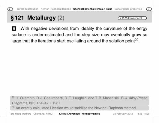
Direct substitution Newton–Raphson iteration Chemical potential versus K -value Convergence properties
15 Multicomponent . . .§ 121 Metallurgy (2)
9 With negative deviations from ideality the curvature of the enrgysurface is under-estimated and the step size may eventually grow solarge that the iterations start oscillating around the solution point20.
19 H. Okamoto, D. J. Chakrabarti, D. E. Laughlin, and T. B. Massalski. Bull. Alloy PhaseDiagrams, 8(5):454–473, 1987.20 An exactly calculated Hessian would stabilise the Newton–Raphson method.
Tore Haug-Warberg (ChemEng, NTNU) KP8108 Advanced Thermodynamics 23 February 2012 833 / 1598

Direct substitution Newton–Raphson iteration Chemical potential versus K -value Convergence properties
0 0.2 0.4 0.6 0.8 1900
950
1000
1050
1100
Tem
pera
ture
[C]
Mole fraction of copper
Figure 15.4: Phase diagram of gold–copper showing a negative deviationfrom ideality. Both TpNewton and TpKvalue has convergence problems closeto the azeotrope.
Tore Haug-Warberg (ChemEng, NTNU) KP8108 Advanced Thermodynamics 23 February 2012 834 / 1598

Direct substitution Newton–Raphson iteration Chemical potential versus K -value Convergence properties
15 Multicomponent . . .First order convergence Consistency1 Concerning the accuracy of the calculations it is not easy to argue
that ∆s⋆i varies over the temperature domain.
2 The simplification which is part of the pure component referenceis dominated by the activity model, and the calculated phase diagramlooks very promising.
3 But, a single phase diagram is not sufficient to claim any kind ofthermodynamic consistency.
4 To do this we have to verify all types of calorimetric quantities,vapour pressures, cryoscopic measurements, etc.
5 A systematic study at this level would indeed reveal the noted in-consistency, as well as several minor ones.
835 / 1598
Morphology1 While azeotropes are common for vapour–liquid phase diagrams,
the analogous phenomena of congruent melting is quite rare among thealloys — at least when disconnected from the formation of stoichiomet-ric solid compounds, or the homogenous phase splitting for one of thephasesa.
2 It has nevertheless been chosen to present an exotic system hereto stress the fact that phase diagrams are classified according to theirmorphology, and that the calculation method is quite independent of thephase models.
3 The thermodynamics of phase equilibria does not make any dif-ference between vapour, liquid and solid phases in this regardb, but inpractise the number of empirical model parameters is often higher inthe description of crystalline phases as compared to the same descrip-tion of vapour and liquid phases of simple organic cmpounds.
4 In the gold–copper case there are e.g. six binary parametersneeded for the solid phases, while only three is needed for the liquid.
836 / 1598
a The gold–copper system exhibits solid phase separation at T < 400 C.b Even though the equilibrium conditions 15.11, 15.15 and 15.19 look quite differently.
1 2 A sequence of iterative calculations has (convergence) order m and(convergence) factor h if the sequence approximates limk→∞ log ‖xk+1−x∞‖ = log(h) + m log ‖xk − x∞‖. The K -value method is typically of first order, but close to the critical
point the convergence factor h → 1 which means xk+1 ≃ xk .
3 Thus, convergence is severely hampered and it may be difficult todecide whether the sequence converges or not.
4 To broaden the applicability of first order methods it has been sug-gested to accelerate the iteration step along the strongest eigendirec-tion of the Jacobi21 matrix. This is known as the Dominant EigenvalueMethod, see Appendix 27.
21 Carl Gustav Jacob Jacobi, 1804–1851. German mathematician.
Tore Haug-Warberg (ChemEng, NTNU) KP8108 Advanced Thermodynamics 23 February 2012 837 / 1598
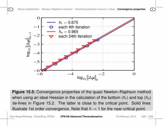
Direct substitution Newton–Raphson iteration Chemical potential versus K -value Convergence properties
−6 −4 −2 0−6
−5
−4
−3
−2
−1
0
log10
∥∥∥∆µ∥∥∥
k
log 1
0
∥ ∥ ∥ ∆µ∥ ∥ ∥ k
+1
h1 = 0.675each 4th iterationhn = 0.965each 24th iteration
Figure 15.5: Convergence properties of the quasi Newton–Raphson methodwhen using an ideal Hessian in the calculation of the bottom (h1) and top (hn)tie-lines in Figure 15.2. The latter is close to the critical point. Solid linesillustrate 1st order convergence. Note that h → 1 for the near-critical point.
Tore Haug-Warberg (ChemEng, NTNU) KP8108 Advanced Thermodynamics 23 February 2012 838 / 1598

Direct substitution Newton–Raphson iteration Chemical potential versus K -value Convergence properties
15 Multicomponent . . .Second order convergence
1 The Newton–Raphson method is of second order — details con-cerning the convergence factor is discussed in Appendix 26.
2 This means that the number of significant digits will double in eachiteration provided that iteration k is sufficiently close to the solutionpoint.
4 3 The local convergence properties are irreproachable, but themethod needs quite good start estimates. But, the simplifications in Section 15.2 makes m = 1 unless for
ideal mixtures where the Hessian is exact.
5 Figure 15.5 illustrates what influence the simplification has on thecalculation of the bottom and top tie-lines of Figure 15.2.
Tore Haug-Warberg (ChemEng, NTNU) KP8108 Advanced Thermodynamics 23 February 2012 839 / 1598

Direct substitution Newton–Raphson iteration Chemical potential versus K -value Convergence properties
15 Multicomponent . . .Second order convergence (2)
6 The iteration sequence approaches a line with slope 1, which istypical for first order methods, and for the near-critical point the conver-gence factor also approaches 1, in the sense that hn = 0.965 is prettyclose to unity in this context.
Tore Haug-Warberg (ChemEng, NTNU) KP8108 Advanced Thermodynamics 23 February 2012 840 / 1598
Global stability Local stability The tangent plane test Intrinsic stability criteria
Part 21
Material Stability
see also Part-Contents
Tore Haug-Warberg (ChemEng, NTNU) KP8108 Advanced Thermodynamics 23 February 2012 1229 / 1598
Global stability Local stability The tangent plane test Intrinsic stability criteria
Contents
1 Global stability
2 Local stability
3 The tangent plane test
1 Lagrange formulation2 Direct substitution
4 Intrinsic stability criteria
Tore Haug-Warberg (ChemEng, NTNU) KP8108 Advanced Thermodynamics 23 February 2012 1230 / 1598

Global stability Local stability The tangent plane test Intrinsic stability criteria
21 Material . . .Note 21.1
1 The question of material stability is crucial to the understandingof complex phase behaviour, and, as an indispensable analytical tool,to the calculation of thermodynamic equilibrium states. It turns out,however, that the subject is quite complex, and that a full theoreticaltreatment requires a rather abstract notation. In order to achieve agood understanding of the basic concepts without sacrificing too muchphysical insight, we will therefore restrict our analysis to U, and possiblyits Legendre transforms A , H and G, but it should be stressed thatsimilar analyses could be carried out based on S, V , etc.
Tore Haug-Warberg (ChemEng, NTNU) KP8108 Advanced Thermodynamics 23 February 2012 1231 / 1598

Global stability Local stability The tangent plane test Intrinsic stability criteria
21 Material . . .Note 21.2
1 Let us start with a closed system held at constant entropy, volumeand composition, the internal energy of which is U(x), where xT = (S ,V ,N1, . . . ,Nn). It is perhaps easier to grasp the theory by looking ata single-phase system. However, this is not a requirement, and nochanges are needed for multi-phase systems. Let us consider whathappens when a new phase, with state variables y ∈ Ω | 0 < y < x, isformed within the system boundary. Of particular interest to us is thechange in internal energy ∆U(x, y) = U(y) + U(x − y) − U(x) causedby the phase formation. A perturbation in U(x) combined with an Eulerintegration of U(y) yields1:
∆U(x, y) = Uy · y − Ux · y + 12! Uxx · y · y − 1
3! Uxxx · y · y · y + . . .
= U +∑
k=2
(−1)k
k ! δk U (21.1)
Tore Haug-Warberg (ChemEng, NTNU) KP8108 Advanced Thermodynamics 23 February 2012 1232 / 1598
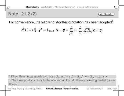
Global stability Local stability The tangent plane test Intrinsic stability criteria
21 Material . . .Note 21.2 (2)
For convenience, the following shorthand notation has been adopted2:
δk U = Ukx · yk = Ux...x · y · · · y =
n∑j=1· · ·
n∑i=1
∂k U∂xi ···∂xj
yi · · · yj
1 Direct Euler integration is also possible: ∆U = (Uy −Ux−y) · y − (Ux − Ux−y) · x2 The inner product · binds to the operand on the left, thereby avoiding nested paren-theses.
Tore Haug-Warberg (ChemEng, NTNU) KP8108 Advanced Thermodynamics 23 February 2012 1233 / 1598
Global stability Local stability The tangent plane test Intrinsic stability criteria
21 Material . . .Note 21.3
1 The tangent plane distance function U = (Uy − Ux) · y defined in21.1 is fundamental to the global stability analysis set out below, whilethe factors δ2U, δ3U, etc. are closely related to the local instabilitiesknown as spinodal, critical, and tricritical points. The exact conditionsfor these states are quite involved, and will be discussed in the nextsection.
Tore Haug-Warberg (ChemEng, NTNU) KP8108 Advanced Thermodynamics 23 February 2012 1234 / 1598

Global stability Local stability The tangent plane test Intrinsic stability criteria
21 Material . . .Note 21.4
1 To prove that the system is in global equilibrium it must be verifiedthat ∆U(x, y) ≥ 0, ∀y ∈ Ω, but it is not necessary to scan the entirefunction domain; the system is globally stable if all the stationary valuesof ∆U have a positive sign. A necessary condition for the stationarystate is (∂∆U/∂y) = 0, which in the current context translates to Uy =
Ux−y3. Substituted into the integrated form of ∆U (see footnote on
page 1163 on Euler integration), this gives the final stability criterion(Uy − Ux) · x ≥ 0, which correctly identifies the equilibrium state as thelowest of all feasible tangent planes. However, this does not give usany clue as to how or where we should start our calculations. Note thatthere may be several phases yi and in general each phase has a finiteregion of attraction4.3 Also referred to as the general condition for phase equilibrium.4 The extent of the region also depends on the numerical algorithm being used.
Tore Haug-Warberg (ChemEng, NTNU) KP8108 Advanced Thermodynamics 23 February 2012 1235 / 1598
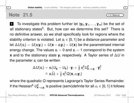
Global stability Local stability The tangent plane test Intrinsic stability criteria
21 Material . . .Note 21.5
1 To investigate this problem further let y0, y1, . . . , ym be the set ofall stationary states5. But, how can we determine this set? There isno definitive answer, so we shall specifically look for regions where thestability criterion is violated. Let si ∈ [0, 1] be a distance parameter andlet ∆U(si) = U(siyi) + U(x − siyi) − U(x) be the parametrised internalenergy change. The values si = 0 and si = 1 correspond to the systemx and to the stationary state yi respectively. A Taylor series of ∆U inthe parameter si can be written
∆U(si) = si(Uyi − Ux) · yi +12 s2
i U2x−αiyi
· y2i
= siUi +12 s2
i Q(x, αiyi)
where the quadratic Q represents Lagrange’s Taylor Series Remainder.If the Hessian6 U2
x−αiyiis positive (semi)definite for all αi ∈ [0, 1] it follows
Tore Haug-Warberg (ChemEng, NTNU) KP8108 Advanced Thermodynamics 23 February 2012 1236 / 1598
Global stability Local stability The tangent plane test Intrinsic stability criteria
21 Material . . .Note 21.5 (2)
that Q is non-negative. Hence, if ∆U(yi) < 0 it must be true that Ui < 0.The reverse is also true because limsi→0 ∆U/si = Ui. The question ofglobal stability can therefore be resolved by calculating min U in eachregion of attraction7:
stable U ≥ 0 ∀yi ∈ Ωmetastable U < 0 ∃yi ∈ Ω
If the tangent plane distance is everywhere non-negative, the system isstable, and if this is not the case, the energy can be lowered by using yi
as an initial estimate for the new phase, see Section 21.3 on page 1185.
5 Any value y ∝ x represents a so-called trivial solution and is excluded from the set.6 Ludwig Otto Hesse, 1811–1874. German mathematician.7 Normally unknown at the outset — global stability constitutes a difficult problem.
Tore Haug-Warberg (ChemEng, NTNU) KP8108 Advanced Thermodynamics 23 February 2012 1237 / 1598
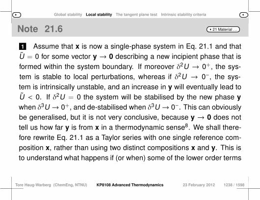
Global stability Local stability The tangent plane test Intrinsic stability criteria
21 Material . . .Note 21.6
1 Assume that x is now a single-phase system in Eq. 21.1 and thatU = 0 for some vector y → 0 describing a new incipient phase that isformed within the system boundary. If moreover δ2U → 0+, the sys-tem is stable to local perturbations, whereas if δ2U → 0−, the sys-tem is intrinsically unstable, and an increase in y will eventually lead toU < 0. If δ2U = 0 the system will be stabilised by the new phase y
when δ3U → 0+, and de-stabilised when δ3U → 0−. This can obviouslybe generalised, but it is not very conclusive, because y → 0 does nottell us how far y is from x in a thermodynamic sense8. We shall there-fore rewrite Eq. 21.1 as a Taylor series with one single reference com-position x, rather than using two distinct compositions x and y. This isto understand what happens if (or when) some of the lower order terms
Tore Haug-Warberg (ChemEng, NTNU) KP8108 Advanced Thermodynamics 23 February 2012 1238 / 1598

Global stability Local stability The tangent plane test Intrinsic stability criteria
21 Material . . .Note 21.6 (2)
in the series vanish, and to properly understand the zero phase fractionlines. The total energy of the composite system is:
U(x, y) = U(y) + U(x − y) (21.2)
8 We do not know whether y approaches the trivial solution y ∝ x or not.
Tore Haug-Warberg (ChemEng, NTNU) KP8108 Advanced Thermodynamics 23 February 2012 1239 / 1598
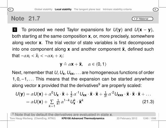
Global stability Local stability The tangent plane test Intrinsic stability criteria
21 Material . . .Note 21.7
1 To proceed we need Taylor expansions for U(y) and U(x − y),both starting at the same composition x, or, more precisely, somewherealong vector x. The trial vector of state variables is first decomposedinto one component along x and another component x, defined suchthat −αxi < xi < −αxi + xi :
y = αx + x, α ∈ 〈0, 1〉Next, remember that U,Ux,Uxx, . . . are homogeneous functions of order1, 0,−1, . . . This means that the expansion can be started anywherealong vector x provided that the derivatives9 are properly scaled:
U(y) = αU(x) + α0Ux · x + 12 α
-1Uxx · x · x + 13! α
-2Uxxx · x · x · x + . . .
= αU(x) +∑
k=1
1k ! α
1−k Ukx · xk (21.3)
9 Note that by default the derivatives are evaluated in state x.Tore Haug-Warberg (ChemEng, NTNU) KP8108 Advanced Thermodynamics 23 February 2012 1240 / 1598

Global stability Local stability The tangent plane test Intrinsic stability criteria
21 Material . . .Note 21.8
1 The expansion of U(y) is also valid for U(x − y) if the new variableβ is defined such that
x − y = x − (αx + x) = (1 − α)x − x = βx − x
Hence, by replacing α→ β and x→ −x we get the expression
U(x − y) = βU(x) +∑
k=1
1k ! β
1−k Ukx · (−x)k (21.4)
for free. From Eqs. 21.2, 21.3 and 21.4 the expansion of the total energyreads10:
U(x, y) = U(x) +∑
k=2
1k !
[α1−k − (−β)1−k
]Uk
x · xk (21.5)
The first index k = 1 is skipped because α0 − β0 = 0 for all α, β ∈ 〈0, 1〉,i.e. the Taylor series is independent of the slope of the energy surface11.Of particular interest here is the term α1−k − (−β)1−k , which is strictly
Tore Haug-Warberg (ChemEng, NTNU) KP8108 Advanced Thermodynamics 23 February 2012 1241 / 1598

Global stability Local stability The tangent plane test Intrinsic stability criteria
21 Material . . .Note 21.8 (2)
positive for the even indices k = 2, 4, . . ., and of variable sign for the oddindices k = 3, 5, . . .. The sign of an odd-powered term can therefore beswitched by exchanging the values of α and β. Whenever the leadingterms of the series vanish, this implies that the even and odd termsvanish in pairs. A concise explanation is given below.
10 Where α+ β = 1, as defined above.11 The energy gained by one phase is, to a first approximation, the same as that lostby the other phase.
Tore Haug-Warberg (ChemEng, NTNU) KP8108 Advanced Thermodynamics 23 February 2012 1242 / 1598
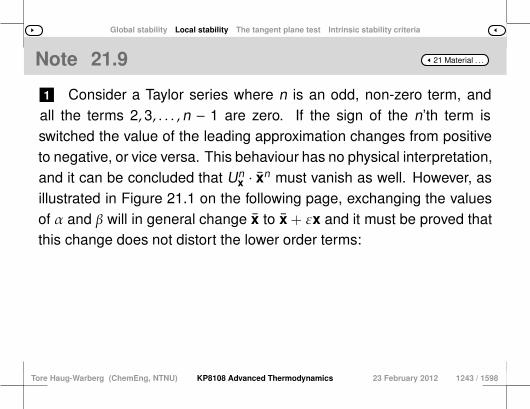
Global stability Local stability The tangent plane test Intrinsic stability criteria
21 Material . . .Note 21.9
1 Consider a Taylor series where n is an odd, non-zero term, andall the terms 2, 3, . . . , n − 1 are zero. If the sign of the n’th term isswitched the value of the leading approximation changes from positiveto negative, or vice versa. This behaviour has no physical interpretation,and it can be concluded that Un
x · xn must vanish as well. However, asillustrated in Figure 21.1 on the following page, exchanging the valuesof α and β will in general change x to x + εx and it must be proved thatthis change does not distort the lower order terms:
Tore Haug-Warberg (ChemEng, NTNU) KP8108 Advanced Thermodynamics 23 February 2012 1243 / 1598
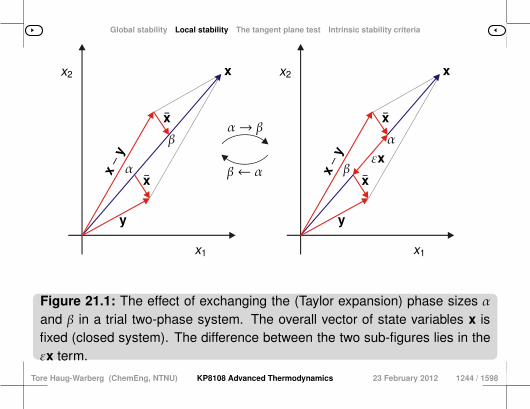
Global stability Local stability The tangent plane test Intrinsic stability criteria
x1x1
x2x2 xx
yy
x
x
x
x
x−
y
x−
y εx
α
α β
βα→ β
β← α
Figure 21.1: The effect of exchanging the (Taylor expansion) phase sizes αand β in a trial two-phase system. The overall vector of state variables x isfixed (closed system). The difference between the two sub-figures lies in theεx term.
Tore Haug-Warberg (ChemEng, NTNU) KP8108 Advanced Thermodynamics 23 February 2012 1244 / 1598
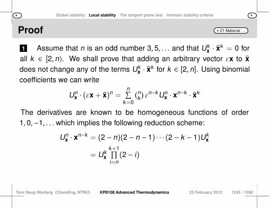
Global stability Local stability The tangent plane test Intrinsic stability criteria
21 Material . . .Proof
1 Assume that n is an odd number 3, 5, . . . and that Ukx · xk = 0 for
all k ∈ [2, n〉. We shall prove that adding an arbitrary vector εx to x
does not change any of the terms Ukx · xk for k ∈ [2, n]. Using binomial
coefficients we can write
Unx · (εx + x)n =
n∑k=0
(nk)εn−k Un
x · xn−k · xk
The derivatives are known to be homogeneous functions of order1, 0,−1, . . . which implies the following reduction scheme:
Unx · xn−k = (2 − n)(2 − n − 1) · · · (2 − k − 1)Uk
x
= Ukx
k+1∏i=n
(2 − i)
Tore Haug-Warberg (ChemEng, NTNU) KP8108 Advanced Thermodynamics 23 February 2012 1245 / 1598
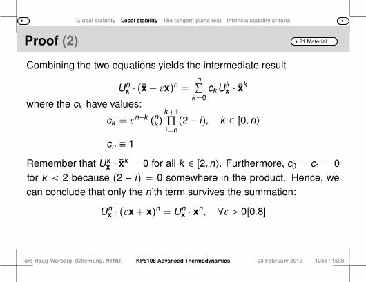
Global stability Local stability The tangent plane test Intrinsic stability criteria
21 Material . . .Proof (2)
Combining the two equations yields the intermediate result
Unx · (x + εx)n =
n∑k=0
ck Ukx · xk
where the ck have values:
ck = εn−k (nk) k+1∏
i=n(2 − i), k ∈ [0, n〉
cn ≡ 1
Remember that Ukx · xk = 0 for all k ∈ [2, n〉. Furthermore, c0 = c1 = 0
for k < 2 because (2 − i) = 0 somewhere in the product. Hence, wecan conclude that only the n’th term survives the summation:
Unx · (εx + x)n = Un
x · xn, ∀ε > 0[0.8]
Tore Haug-Warberg (ChemEng, NTNU) KP8108 Advanced Thermodynamics 23 February 2012 1246 / 1598
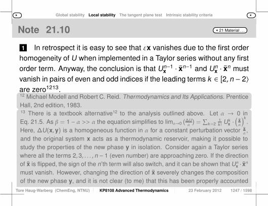
Global stability Local stability The tangent plane test Intrinsic stability criteria
21 Material . . .Note 21.10
1 In retrospect it is easy to see that εx vanishes due to the first orderhomogeneity of U when implemented in a Taylor series without any firstorder term. Anyway, the conclusion is that Un−1
x · xn−1 and Unx · xn must
vanish in pairs of even and odd indices if the leading terms k ∈ [2, n − 2〉are zero1213.12 Michael Modell and Robert C. Reid. Thermodynamics and Its Applications. PrenticeHall, 2nd edition, 1983.13 There is a textbook alternative12 to the analysis outlined above. Let α → 0 inEq. 21.5. As β = 1 − α >> α the equation simplifies to limα→0 (
∆Uα) =
∑k=2
1k ! Uk
x ·(
xα
)k.
Here, ∆U(x,y) is a homogeneous function in α for a constant perturbation vector xα ,
and the original system x acts as a thermodynamic reservoir, making it possible tostudy the properties of the new phase y in isolation. Consider again a Taylor serieswhere all the terms 2,3, . . . , n − 1 (even number) are approaching zero. If the directionof x is flipped, the sign of the n’th term will also switch, and it can be shown that Un
x · xn
must vanish. However, changing the direction of x severely changes the compositionof the new phase y, and it is not clear (to me) that this has been properly accountedfor in the analysis. I therefore find this argument weaker than my own.Tore Haug-Warberg (ChemEng, NTNU) KP8108 Advanced Thermodynamics 23 February 2012 1247 / 1598
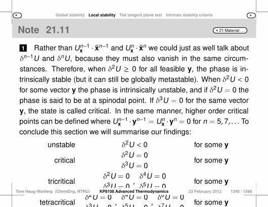
Global stability Local stability The tangent plane test Intrinsic stability criteria
21 Material . . .Note 21.11
1 Rather than Un−1x · xn−1 and Un
x · xn we could just as well talk aboutδn−1U and δnU, because they must also vanish in the same circum-stances. Therefore, when δ2U ≥ 0 for all feasible y, the phase is in-trinsically stable (but it can still be globally metastable). When δ2U < 0for some vector y the phase is intrinsically unstable, and if δ2U = 0 thephase is said to be at a spinodal point. If δ3U = 0 for the same vectory, the state is called critical. In the same manner, higher order criticalpoints can be defined where Un−1
x · yn−1 = Unx · yn = 0 for n = 5, 7, . . . To
conclude this section we will summarise our findings:
unstable δ2U < 0 for some y
criticalδ2U = 0δ3U = 0
for some y
tricriticalδ2U = 0δ3U = 0
,δ4U = 0δ5U = 0
for some y
tetracriticalδ2U = 0δ3U = 0
,δ4U = 0δ5U = 0
,δ6U = 0δ7U = 0
for some y
Tore Haug-Warberg (ChemEng, NTNU) KP8108 Advanced Thermodynamics 23 February 2012 1248 / 1598

Global stability Local stability The tangent plane test Intrinsic stability criteria
21 Material . . .Note 21.11 (2)
Tore Haug-Warberg (ChemEng, NTNU) KP8108 Advanced Thermodynamics 23 February 2012 1249 / 1598
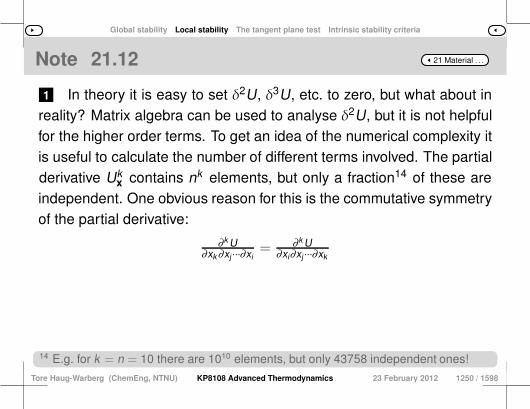
Global stability Local stability The tangent plane test Intrinsic stability criteria
21 Material . . .Note 21.12
1 In theory it is easy to set δ2U, δ3U, etc. to zero, but what about inreality? Matrix algebra can be used to analyse δ2U, but it is not helpfulfor the higher order terms. To get an idea of the numerical complexity itis useful to calculate the number of different terms involved. The partialderivative Uk
x contains nk elements, but only a fraction14 of these areindependent. One obvious reason for this is the commutative symmetryof the partial derivative:
∂k U∂xk∂xj ···∂xi
= ∂k U∂xi∂xj ···∂xk
14 E.g. for k = n = 10 there are 1010 elements, but only 43758 independent ones!
Tore Haug-Warberg (ChemEng, NTNU) KP8108 Advanced Thermodynamics 23 February 2012 1250 / 1598

Global stability Local stability The tangent plane test Intrinsic stability criteria
21 Material . . .Note 21.13
1 Thus, the sampling of k indices without regard to order from apopulation of n = dim(x) components (with replacement of the indices)gives rise to
(n+k−1k
) ≡ (n+k−1)!k !(n−1)!
potentially different terms in Ukx . However, the homogeneity of U re-
duces the number further because
Ukx · x = (2 − k)Uk−1
x
For each derivative Ukx there exist as many relations as there are inde-
pendent terms in Uk−1x , hence the number of independent terms in Uk
x
is limited to(n+k−1
k) − (n+k−2
k−1) ≡ (n+k−2)!
k !(n−2)! , k , n ≥ 2
Tore Haug-Warberg (ChemEng, NTNU) KP8108 Advanced Thermodynamics 23 February 2012 1251 / 1598

Global stability Local stability The tangent plane test Intrinsic stability criteria
21 Material . . .Note 21.14
1 From the numbers calculated in the table below we can immedi-ately identify the 2-variable case as particularly interesting — only oneextra term is needed to describe each derivative, regardless of the valueof k . This finding becomes even more interesting in Section 21.4, wherewe will find that the 2-variable case is sufficient in all but some highlydegenerate cases (e.g. critical azeotropes).
k = 2 k = 3 k = 4 · · · k
n = 2 1 1 1 · · · 11
n = 3 3 4 5 · · · k+11
n = 4 6 10 15 · · · (k+1)(k+2)2
......
......
. . ....
n (n−1)n2
(n−1)n(n+1)6
(n−1)n(n+1)(n+2)24 · · · (n+k−2)!
k !(n−2)!
Tore Haug-Warberg (ChemEng, NTNU) KP8108 Advanced Thermodynamics 23 February 2012 1252 / 1598

Global stability Local stability The tangent plane test Intrinsic stability criteria
21 Material . . .Note 21.14 (2)
Tore Haug-Warberg (ChemEng, NTNU) KP8108 Advanced Thermodynamics 23 February 2012 1253 / 1598
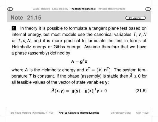
Global stability Local stability The tangent plane test Intrinsic stability criteria
21 Material . . .Note 21.15
1 In theory it is possible to formulate a tangent plane test based oninternal energy, but most models use the canonical variables T ,V ,Nor T , p,N, and it is more practical to formulate the test in terms ofHelmholtz energy or Gibbs energy. Assume therefore that we havea phase (assembly) defined by
A = gTx
where A is the Helmholtz energy and xT = (V , nT). The system tem-perature T is constant. If the phase (assembly) is stable then A ≥ 0 forall feasible values of the vector of state variables y:
A(x, y) = [g(y) − g(x)]Ty > 0 (21.6)
Tore Haug-Warberg (ChemEng, NTNU) KP8108 Advanced Thermodynamics 23 February 2012 1254 / 1598
Global stability Local stability The tangent plane test Intrinsic stability criteria
21 Material . . .Note 21.15 (2)
Note the difference in notation from Eq. 21.1. Here it is more natural touse g for the gradient rather than Ax, in keeping with the notation usedin linear algebra.
Tore Haug-Warberg (ChemEng, NTNU) KP8108 Advanced Thermodynamics 23 February 2012 1255 / 1598

Global stability Local stability The tangent plane test Intrinsic stability criteria
21 Material . . .Note 21.16
1 To verify that A ≥ 0 for all feasible y ∈ Ω our best option is toinvestigate the outcome of the minimisation problem
miny
(A)T ∨ aTy = c
for several trial values of y. This minimisation problem is linearly con-strained15 and the method of Lagrange multipliers is the perfect tool:
L(x, y, λ) = A − λ(aTy − c)
15 The constraint specification aTy = c is arbitrary, but nevertheless crucial to theformulation of the problem, because A is a homogeneous function, and as such has asingular Hessian matrix in the direction of y. Adding a rank-one constraint makes theHessian invertible (loosely speaking).
Tore Haug-Warberg (ChemEng, NTNU) KP8108 Advanced Thermodynamics 23 February 2012 1256 / 1598

Global stability Local stability The tangent plane test Intrinsic stability criteria
21 Material . . .Note 21.17
1 The stationary point of L is given by ∂L/∂y = 0, or when writtenout in more detail:
0 = ∂A∂y− ∂λ(aTy−c)
∂y
= H(y)y + g(y) − g(x) − λa
= g(y) − g(x) − λa (21.7)
The stationary value of A can be calculated from Eqs. 21.6 and 21.7:
A = g(y)Ty − g(x)Ty = λaTy = λc (21.8)
Tore Haug-Warberg (ChemEng, NTNU) KP8108 Advanced Thermodynamics 23 February 2012 1257 / 1598

Global stability Local stability The tangent plane test Intrinsic stability criteria
21 Material . . .Note 21.18
1 Hence, the phase is stable if λc ≥ 0 at every stationary point ofL(x, y, λ), and metastable if λc < 0. If metastability occurs, Helmholtzenergy can be lowered by including the new phase y at the expenseof x, but this begs the question: how big should we make this newphase? The final answer lies, of course, in the subsequent equilibriumcalculation, but we have to start the iterations somewhere. It requiresonly a minimum of effort to study the second order variation of A alongthe (optimum) vector of state variables y,
A(x, y) = αg(y)Ty − αg(x)Ty + α2
2! yTH(x)y + . . .
Tore Haug-Warberg (ChemEng, NTNU) KP8108 Advanced Thermodynamics 23 February 2012 1258 / 1598

Global stability Local stability The tangent plane test Intrinsic stability criteria
21 Material . . .Note 21.18 (2)
where α ∈ [0, αmax〉 is a step length parameter under our control. A min-imum in Helmholtz energy requires that ∂A/∂α = 0 and simple differen-tiation gives the following phase size estimate
α =g(y)Ty−g(x)Ty
yTH(x)y= −λc
Q(x,y) (21.9)
Tore Haug-Warberg (ChemEng, NTNU) KP8108 Advanced Thermodynamics 23 February 2012 1259 / 1598
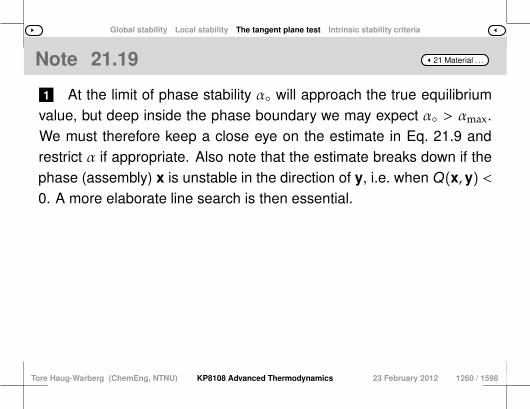
Global stability Local stability The tangent plane test Intrinsic stability criteria
21 Material . . .Note 21.19
1 At the limit of phase stability α will approach the true equilibriumvalue, but deep inside the phase boundary we may expect α > αmax.We must therefore keep a close eye on the estimate in Eq. 21.9 andrestrict α if appropriate. Also note that the estimate breaks down if thephase (assembly) x is unstable in the direction of y, i.e. when Q(x, y) <
0. A more elaborate line search is then essential.
Tore Haug-Warberg (ChemEng, NTNU) KP8108 Advanced Thermodynamics 23 February 2012 1260 / 1598
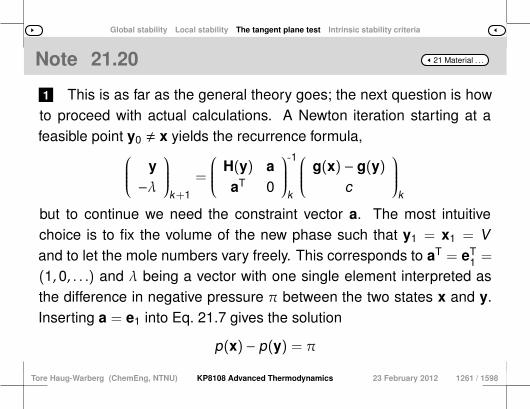
Global stability Local stability The tangent plane test Intrinsic stability criteria
21 Material . . .Note 21.20
1 This is as far as the general theory goes; the next question is howto proceed with actual calculations. A Newton iteration starting at afeasible point y0 , x yields the recurrence formula,
y
−λ
k+1
=
H(y) a
aT 0
-1
k
g(x) − g(y)
c
k
but to continue we need the constraint vector a. The most intuitivechoice is to fix the volume of the new phase such that y1 = x1 = Vand to let the mole numbers vary freely. This corresponds to aT = eT
1 =
(1, 0, . . .) and λ being a vector with one single element interpreted asthe difference in negative pressure π between the two states x and y.Inserting a = e1 into Eq. 21.7 gives the solution
p(x) − p(y) = π
Tore Haug-Warberg (ChemEng, NTNU) KP8108 Advanced Thermodynamics 23 February 2012 1261 / 1598

Global stability Local stability The tangent plane test Intrinsic stability criteria
21 Material . . .Note 21.20 (2)
µ(x) − µ(y) = 0
Tore Haug-Warberg (ChemEng, NTNU) KP8108 Advanced Thermodynamics 23 February 2012 1262 / 1598
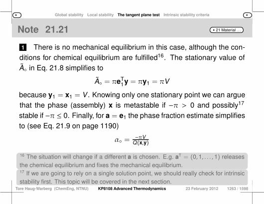
Global stability Local stability The tangent plane test Intrinsic stability criteria
21 Material . . .Note 21.21
1 There is no mechanical equilibrium in this case, although the con-ditions for chemical equilibrium are fulfilled16. The stationary value ofA in Eq. 21.8 simplifies to
A = πeT1y = πy1 = πV
because y1 = x1 = V . Knowing only one stationary point we can arguethat the phase (assembly) x is metastable if −π > 0 and possibly17
stable if −π ≤ 0. Finally, for a = e1 the phase fraction estimate simplifiesto (see Eq. 21.9 on page 1190)
α = −πVQ(x,y)
16 The situation will change if a different a is chosen. E.g. aT = (0,1, . . . , 1) releasesthe chemical equilibrium and fixes the mechanical equilibrium.17 If we are going to rely on a single solution point, we should really check for intrinsicstability first. This topic will be covered in the next section.
Tore Haug-Warberg (ChemEng, NTNU) KP8108 Advanced Thermodynamics 23 February 2012 1263 / 1598
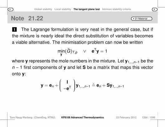
Global stability Local stability The tangent plane test Intrinsic stability criteria
21 Material . . .Note 21.22
1 The Lagrange formulation is very neat in the general case, but ifthe mixture is nearly ideal the direct substitution of variables becomesa viable alternative. The minimisation problem can now be written
miny
(G)T ,p ∨ eTy = 1
where y represents the mole numbers in the mixture. Let y1,...,n−1 be then − 1 first components of y and let S be a matrix that maps this vectoronto y:
y = en +
I
−eT
y1,...,n−1 = en + Sy1,...,n−1
Tore Haug-Warberg (ChemEng, NTNU) KP8108 Advanced Thermodynamics 23 February 2012 1264 / 1598

Global stability Local stability The tangent plane test Intrinsic stability criteria
21 Material . . .Note 21.23
1 The variation in y is easily calculated as δy = Sδy1,...,n−1, andbecause eTS = 0T it follows that eTδy = 0. Clearly, this operationconserves the total number of moles in the mixture and the minimi-sation problem can de facto be written in an unconstrained form asminy1,...,n−1(G)T ,p. The chain rule of differentiation yields
( ∂G∂y1,...,n−1
)=
( ∂nT
∂y1,...,n−1
) (∂G∂y
)= ST[µ(y) − µ(x)] = 0
Tore Haug-Warberg (ChemEng, NTNU) KP8108 Advanced Thermodynamics 23 February 2012 1265 / 1598
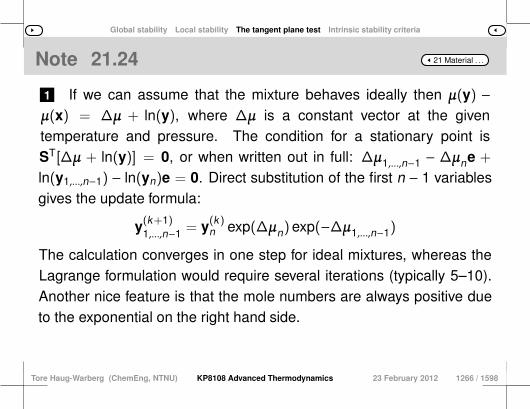
Global stability Local stability The tangent plane test Intrinsic stability criteria
21 Material . . .Note 21.24
1 If we can assume that the mixture behaves ideally then µ(y) −µ(x) = ∆µ + ln(y), where ∆µ is a constant vector at the giventemperature and pressure. The condition for a stationary point isST[∆µ + ln(y)] = 0, or when written out in full: ∆µ1,...,n−1 − ∆µne +
ln(y1,...,n−1) − ln(yn)e = 0. Direct substitution of the first n − 1 variablesgives the update formula:
y(k+1)1,...,n−1 = y
(k)n exp(∆µn)exp(−∆µ1,...,n−1)
The calculation converges in one step for ideal mixtures, whereas theLagrange formulation would require several iterations (typically 5–10).Another nice feature is that the mole numbers are always positive dueto the exponential on the right hand side.
Tore Haug-Warberg (ChemEng, NTNU) KP8108 Advanced Thermodynamics 23 February 2012 1266 / 1598
Global stability Local stability The tangent plane test Intrinsic stability criteria
21 Material . . .§ 153 § 152 § 1
Write a modified update formula for the direct substitutionof mole numbers in an ideal gas at fixed temperature.
The volume is a free variable and can be set to any value.
Tore Haug-Warberg (ChemEng, NTNU) KP8108 Advanced Thermodynamics 23 February 2012 1267 / 1598
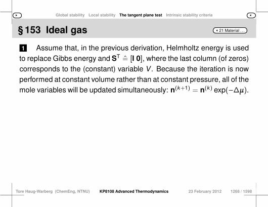
Global stability Local stability The tangent plane test Intrinsic stability criteria
21 Material . . .§ 153 Ideal gas
1 Assume that, in the previous derivation, Helmholtz energy is usedto replace Gibbs energy and ST = [I 0], where the last column (of zeros)corresponds to the (constant) variable V . Because the iteration is nowperformed at constant volume rather than at constant pressure, all of themole variables will be updated simultaneously: n(k+1) = n(k) exp(−∆µ).
Tore Haug-Warberg (ChemEng, NTNU) KP8108 Advanced Thermodynamics 23 February 2012 1268 / 1598
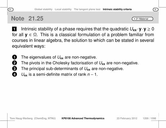
Global stability Local stability The tangent plane test Intrinsic stability criteria
21 Material . . .Note 21.25
1 Intrinsic stability of a phase requires that the quadratic Uxx ·y ·y ≥ 0for all y ∈ Ω. This is a classical formulation of a problem familiar fromcourses in linear algebra, the solution to which can be stated in severalequivalent ways:
1 The eigenvalues of Uxx are non-negative.2 The pivots in the Cholesky factorisation of Uxx are non-negative.3 The principal sub-determinants of Uxx are non-negative.4 Uxx is a semi-definite matrix of rank n − 1.
Tore Haug-Warberg (ChemEng, NTNU) KP8108 Advanced Thermodynamics 23 February 2012 1269 / 1598

Global stability Local stability The tangent plane test Intrinsic stability criteria
21 Material . . .Note 21.26
1 The second formulation is suited to simple matrix algebra and forthis reason it is the route followed here. For a single-component systema step-by-step elimination18 of the rows in Uxx yields
USS USV USN
UVS UVV UVN
UNS UNV UNN
=
1 0 0α 1 0β 0 1
USS USV USN
0 AVV AVN
0 ANV ANN
(21.10)
=
1 0 0α 1 0β γ 1
USS USV USN
0 AVV AVN
0 0 GNN
(21.11)
where the following parameters have been used:
α =UVSUSS
, β = UNSUSS
, γ = ANVAVV
18 Because Uxx is a symmetric matrix of rank n − 1 we can write the full Choleskyfactorisation of an intrinsically stable, single-component system, as Uxx = LLT whereLT =
(u uα uβ0 a aγ
)and u =
√USS and a =
√AVV
Tore Haug-Warberg (ChemEng, NTNU) KP8108 Advanced Thermodynamics 23 February 2012 1270 / 1598

Global stability Local stability The tangent plane test Intrinsic stability criteria
21 Material . . .Note 21.27
1 Note that the last pivot in the elimination (GNN in this case) willalways be 0 due to the homogeneous nature of U. To prove thatEqs. 21.10–21.11 are correct, we must prove that the Cholesky19 fac-torisation of a thermodynamic Hessian (in the extensive variables) isequivalent to a series of Legendre transformations applied to the origi-nal function20. It is possible to prove this in general terms, but to makethe theory more accessible to the casual reader we shall carry out aless general factorisation. From Chapter 4 we know that A(T ,V ,N) isrelated to U(S ,V ,N) such that AX = UX , assuming constant temper-ature and entropy respectively. This relation holds for any X ∈ V ,N.
Tore Haug-Warberg (ChemEng, NTNU) KP8108 Advanced Thermodynamics 23 February 2012 1271 / 1598
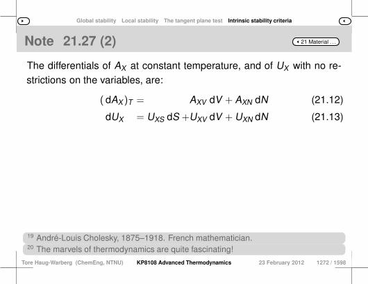
Global stability Local stability The tangent plane test Intrinsic stability criteria
21 Material . . .Note 21.27 (2)
The differentials of AX at constant temperature, and of UX with no re-strictions on the variables, are:
(dAX )T = AXV dV + AXN dN (21.12)
dUX = UXS dS +UXV dV + UXN dN (21.13)
19 André-Louis Cholesky, 1875–1918. French mathematician.20 The marvels of thermodynamics are quite fascinating!
Tore Haug-Warberg (ChemEng, NTNU) KP8108 Advanced Thermodynamics 23 February 2012 1272 / 1598

Global stability Local stability The tangent plane test Intrinsic stability criteria
21 Material . . .Note 21.28
1 In order to compare the two differentials it is necessary to eliminatethe (differential) entropy in the second equation such that the tempera-ture is held constant. Using the definition T = US it follows that
0 = (dUS)T = USS dS + USV dV + USN dN (21.14)
From Eq. 21.14 it is straightforward to eliminate dS in Eq. 21.13, andfurthermore to collect similar terms into
(dUX)T =(UXV − UXS
USVUSS
)dV +
(UXN − UXS
USNUSS
)dN
Tore Haug-Warberg (ChemEng, NTNU) KP8108 Advanced Thermodynamics 23 February 2012 1273 / 1598

Global stability Local stability The tangent plane test Intrinsic stability criteria
21 Material . . .Note 21.29
1 The above equation can be compared term-by-term with Eq. 21.12,which yields
AXY = UXY − UXSUSYUSS
(21.15)
for any Y ∈ V ,N. Substitution of X ,Y ∈ V ,N into the formula aboveverifies the first step of the Cholesky factorisation 21.10–21.11. Further-more, because the differentiation outlined in Eqs. 21.12–21.15 is validfor any Legendre sequence U(S ,V ,N) → A(T ,V ,N) → G(T ,−p,N)
etc., proof by induction verifies that the factorisation can be completedas indicated21.21 The factorisation of positive semi-definite matrices has not yet been discussed.The question is where the zero pivots of Uxx appear when a stable phase changes(continuously) into an unstable one. The outcome is that the last pivot changes its signbefore the second last pivot does, which in turn changes its sign before the third lastpivot, etc. This holds for all non-degenerate states. In the current case GNN = 0 is thelast pivot and the sign shift will therefore show up in AVV first, before it eventually alsoshows up in USS .
Tore Haug-Warberg (ChemEng, NTNU) KP8108 Advanced Thermodynamics 23 February 2012 1274 / 1598
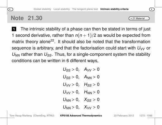
Global stability Local stability The tangent plane test Intrinsic stability criteria
21 Material . . .Note 21.30
1 The intrinsic stability of a phase can then be stated in terms of just1 second derivative, rather than n(n + 1)/2 as would be expected frommatrix theory alone22. It should also be noted that the transformationsequence is arbitrary, and that the factorisation could start with UVV orUNN rather than USS . Thus, for a single-component system the stabilityconditions can be written in 6 different ways,
USS > 0, AVV > 0
USS > 0, ANN > 0
UVV > 0, HSS > 0
UVV > 0, HNN > 0
UNN > 0, XSS > 0
UNN > 0, XVV > 0
Tore Haug-Warberg (ChemEng, NTNU) KP8108 Advanced Thermodynamics 23 February 2012 1275 / 1598
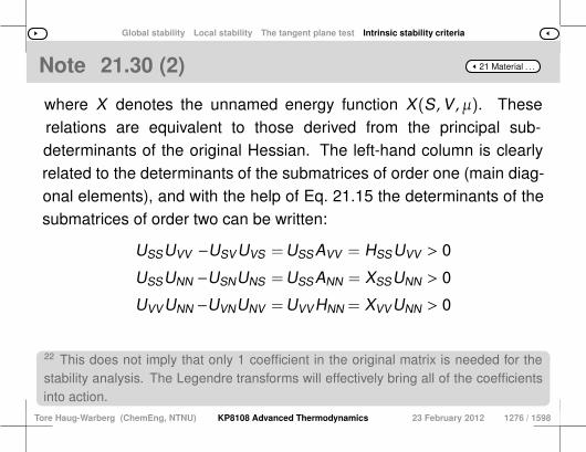
Global stability Local stability The tangent plane test Intrinsic stability criteria
21 Material . . .Note 21.30 (2)
where X denotes the unnamed energy function X(S ,V , µ). Theserelations are equivalent to those derived from the principal sub-determinants of the original Hessian. The left-hand column is clearlyrelated to the determinants of the submatrices of order one (main diag-onal elements), and with the help of Eq. 21.15 the determinants of thesubmatrices of order two can be written:
USSUVV −USVUVS =USSAVV = HSSUVV > 0
USSUNN −USNUNS =USSANN = XSSUNN > 0
UVVUNN −UVNUNV =UVVHNN = XVVUNN > 0
22 This does not imply that only 1 coefficient in the original matrix is needed for thestability analysis. The Legendre transforms will effectively bring all of the coefficientsinto action.
Tore Haug-Warberg (ChemEng, NTNU) KP8108 Advanced Thermodynamics 23 February 2012 1276 / 1598
Global stability Local stability The tangent plane test Intrinsic stability criteria
21 Material . . .Note 21.31
1 There is also one final criterion relating to the whole matrix, andseveral additional criteria from the Legendre transforms, but they are allzero because the Hessian is singular for any values of S, V and N. Thecriteria given in the right-hand column above are therefore conclusiveand are violated simultaneously at the limit of material stability. Thislimit of stability is often referred to as the spinodal. The criteria derivedfrom the submatrices of order one define a new spinodal inside theouter one.
Tore Haug-Warberg (ChemEng, NTNU) KP8108 Advanced Thermodynamics 23 February 2012 1277 / 1598
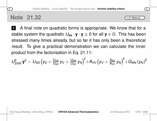
Global stability Local stability The tangent plane test Intrinsic stability criteria
21 Material . . .Note 21.32
1 A final note on quadratic forms is appropriate. We know that for astable system the quadratic Uxx · y · y ≥ 0 for all y ∈ Ω. This has beenstressed many times already, but so far it has only been a theoreticalresult. To give a practical demonstration we can calculate the innerproduct from the factorisation in Eq. 21.11:
U2SVN ·y
2 = USS
(yS +
UVSUSS
yV +UNSUSS
yN
)2+AVV
(yV + ANV
AVVyN
)2+GNN (yN)
2
Tore Haug-Warberg (ChemEng, NTNU) KP8108 Advanced Thermodynamics 23 February 2012 1278 / 1598
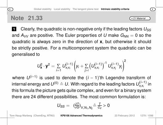
Global stability Local stability The tangent plane test Intrinsic stability criteria
21 Material . . .Note 21.33
1 Clearly, the quadratic is non-negative only if the leading factors USS
and AVV are positive. The Euler properties of U make GNN = 0 so thequadratic is always zero in the direction of x, but otherwise it shouldbe strictly positive. For a multicomponent system the quadratic can begeneralised to
U2x · y2 =
∑i=1
U(i−1)xixi
(yi +
∑j>i
(U(i−1)
xixi
)-1U(i−1)
xixjyj
)2
where U(i−1) is used to denote the (i − 1)’th Legendre transform ofinternal energy and U(0) = U. With regard to the leading factors U(i−1)
xixiin
this formula the picture gets quite complex, and even for a binary systemthere are 24 different possibilities. The most common formulation is:
USS =(∂T∂S
)V ,N1,N2
= TCV> 0
Tore Haug-Warberg (ChemEng, NTNU) KP8108 Advanced Thermodynamics 23 February 2012 1279 / 1598
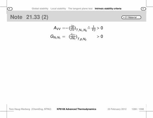
Global stability Local stability The tangent plane test Intrinsic stability criteria
21 Material . . .Note 21.33 (2)
AVV =− (∂p∂V
)T ,N1,N2
= 1Vβ > 0
GN1N1 =(∂µ1
∂N1
)T ,p,N2
> 0
Tore Haug-Warberg (ChemEng, NTNU) KP8108 Advanced Thermodynamics 23 February 2012 1280 / 1598
Related Documents