Lecture Notes in Economic Growth Christian Groth February 11, 2016

Welcome message from author
This document is posted to help you gain knowledge. Please leave a comment to let me know what you think about it! Share it to your friends and learn new things together.
Transcript
Lecture Notes in Economic Growth
Christian Groth
February 11, 2016

ii
c° Groth, Lecture notes in Economic Growth, (mimeo) 2016.
Preface
This is a slight extension of my lecture notes in Economic Growth from 2015.
These notes have been used in recent years in the course Economic Growth
within the Master’s Program in Economics at the Department of Economics,
University of Copenhagen. Discovered typos and similar have been corrected.
In some of the chapters a terminal list of references is included, in some not.
The lecture notes contain many references to the textbook by Daron
Acemoglu, Introduction to Modern Economic Growth (Princeton University
Press, 2009). Parts of the lecture notes are alternative presentations of stuff
also covered in the Acemoglu book, while other parts can be seen as com-
plementary. Sections marked by an asterisk, *, can be skipped, at least in a
first reading.
For constructive criticism I thank Niklas Brønager, class instructor since
2012, and plenty of earlier students. No doubt, obscurities remain. Hence, I
very much welcome comments and suggestions of any kind relating to these
lecture notes.
February 2016
Christian Groth
ix

x PREFACE
c° Groth, Lecture notes in Economic Growth, (mimeo) 2016.
Chapter 1
Introduction to economic
growth
This introductory lecture note is a refresher on basic concepts.
Section 1.1 defines Economic Growth as a field of economics. In Section
1.2 formulas for calculation of compound average growth rates in discrete and
continuous time are presented. Section 1.3 briefly presents two sets of what
is by many considered as “stylized facts” about economic growth. Finally,
Section 1.4 discusses, in an informal way, the different concepts of cross-
country income convergence. In his introductory Chapter 1, §1.5, Acemoglu1
briefly touches upon these concepts.
1.1 The field
Economic growth analysis is the study of what factors and mechanisms deter-
mine the time path of productivity (a simple index of productivity is output
per unit of labor). The focus is on
• productivity levels and
• productivity growth.
1.1.1 Economic growth theory
Economic growth theory endogenizes productivity growth via considering
human capital accumulation (formal education as well as learning-by-doing)
1Throughout these lecture notes, “Acemoglu” refers to Daron Acemoglu, Introduction
to Modern Economic Growth, Princeton University Press: Oxford, 2009.
1
2 CHAPTER 1. INTRODUCTION TO ECONOMIC GROWTH
and endogenous research and development. Also the conditioning role of
geography and juridical, political, and cultural institutions is taken into ac-
count.
For practical reasons, economic growth theory is often stated in terms of
national income and product account variables like per capita GDP. Yet the
term “economic growth” may be interpreted as referring to something deeper.
We could think of “economic growth” as the widening of the opportunities
of human beings to lead a freer and more worthwhile life (cf. Sen, ....).
To make our complex economic environment accessible for theoretical
analysis we use economic models. What is an economic model? It is a way
of organizing one’s thoughts about the economic functioning of a society. A
more specific answer is to define an economic model as a conceptual struc-
ture based on a set of mathematically formulated assumptions which have
an economic interpretation and from which empirically testable predictions
can be derived. In particular, an economic growth model is an economic
model concerned with productivity issues. The union of connected and non-
contradictory models dealing with economic growth and the propositions
derived from these models constitute economic growth theory. Occasionally,
intense controversies about the validity of alternative growth theories take
place.
The terms “New Growth Theory” and “endogenous growth theory” re-
fer to theory and models which attempt at explaining sustained per capita
growth as an outcome of internal mechanisms in the model rather than just
a reflection of exogenous technical progress as in “Old Growth Theory”.
Among the themes addressed in this course are:
• How is the world income distribution evolving?• Why do living standards differ so much across countries and regions?Why are some countries 50 times richer than others?
• Why do per capita growth rates differ over long periods?• What are the roles of human capital and technology innovation in eco-nomic growth? Getting the questions right.
• Catching-up and increased speed of communication and technology dif-fusion.
• Economic growth, natural resources, and the environment (includingthe climate). What are the limits to growth?
• Policies to ignite and sustain productivity growth.
c° Groth, Lecture notes in Economic Growth, (mimeo) 2016.
1.1. The field 3
• The prospects of growth in the future.
The course concentrates on mechanisms behind the evolution of produc-
tivity in the industrialized world. We study these mechanisms as integral
parts of dynamic models.
The exam is a test of the extent to which the student has acquired under-
standing of these models, is able to evaluate them, from both a theoretical
and empirical perspective, and is able to use them to analyze specific eco-
nomic questions. The course is calculus intensive.
1.1.2 Some long-run data
Let denote real GDP (per year) and let be population size. Then
is GDP per capita. Further, let denote the average (compound) growth
rate of per year since 1870 and let denote the average (compound)
growth rate of per year since 1870. Table 1.1 gives these growth rates
for four countries. (But we should not forget that data from before WWII
should be taken with a grain of salt).
Denmark 2,67 1,87
UK 1,96 1,46
USA 3,40 1,89
Japan 3,54 2,54
Table 1.1: Average annual growth rate of GDP and GDP per capita in percent,
1870—2006. Discrete compounding. Source: Maddison, A: The World Economy:
Historical Statistics, 2006, Table 1b, 1c and 5c.
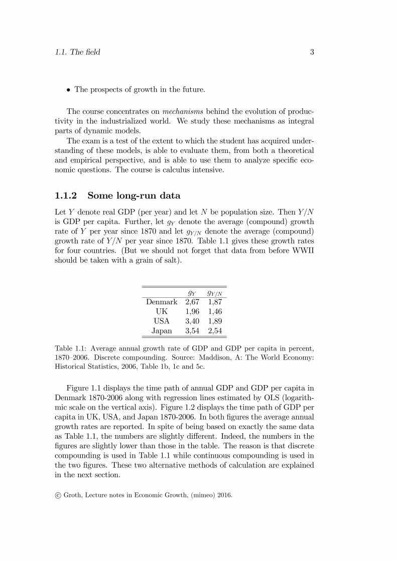
Figure 1.1 displays the time path of annual GDP and GDP per capita in
Denmark 1870-2006 along with regression lines estimated by OLS (logarith-
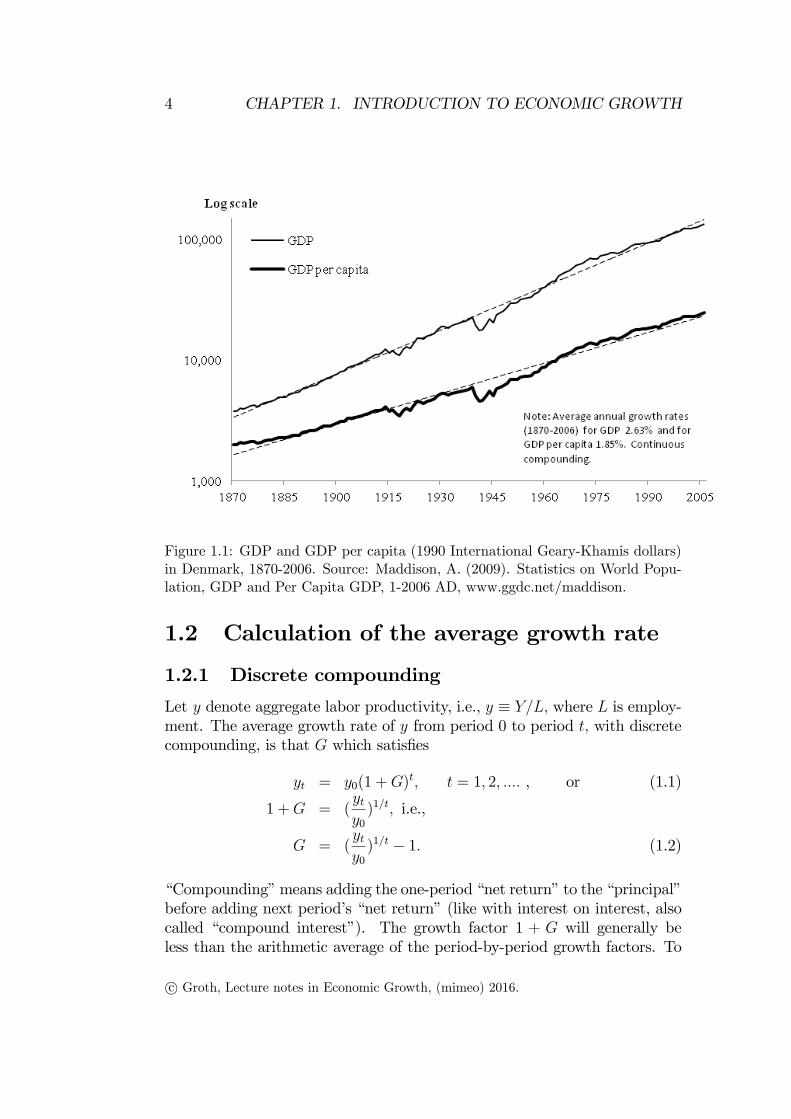
mic scale on the vertical axis). Figure 1.2 displays the time path of GDP per
capita in UK, USA, and Japan 1870-2006. In both figures the average annual
growth rates are reported. In spite of being based on exactly the same data
as Table 1.1, the numbers are slightly different. Indeed, the numbers in the
figures are slightly lower than those in the table. The reason is that discrete
compounding is used in Table 1.1 while continuous compounding is used in
the two figures. These two alternative methods of calculation are explained
in the next section.
c° Groth, Lecture notes in Economic Growth, (mimeo) 2016.
4 CHAPTER 1. INTRODUCTION TO ECONOMIC GROWTH
Figure 1.1: GDP and GDP per capita (1990 International Geary-Khamis dollars)
in Denmark, 1870-2006. Source: Maddison, A. (2009). Statistics on World Popu-
lation, GDP and Per Capita GDP, 1-2006 AD, www.ggdc.net/maddison.
1.2 Calculation of the average growth rate
1.2.1 Discrete compounding
Let denote aggregate labor productivity, i.e., ≡ where is employ-
ment. The average growth rate of from period 0 to period with discrete
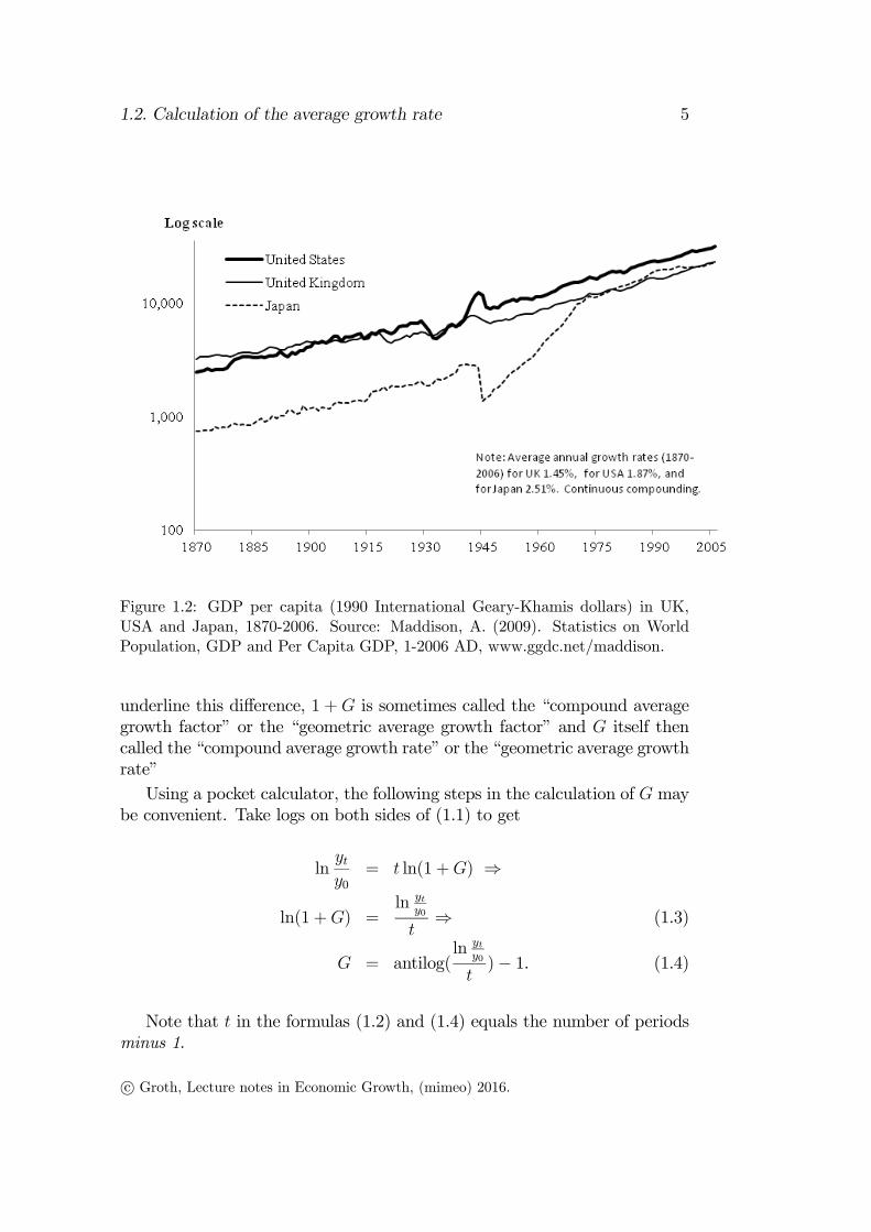
compounding, is that which satisfies
= 0(1 +) = 1 2 , or (1.1)
1 + = (
0)1 i.e.,
= (
0)1 − 1 (1.2)
“Compounding” means adding the one-period “net return” to the “principal”
before adding next period’s “net return” (like with interest on interest, also
called “compound interest”). The growth factor 1 + will generally be
less than the arithmetic average of the period-by-period growth factors. To
c° Groth, Lecture notes in Economic Growth, (mimeo) 2016.
1.2. Calculation of the average growth rate 5
Figure 1.2: GDP per capita (1990 International Geary-Khamis dollars) in UK,
USA and Japan, 1870-2006. Source: Maddison, A. (2009). Statistics on World
Population, GDP and Per Capita GDP, 1-2006 AD, www.ggdc.net/maddison.
underline this difference, 1 + is sometimes called the “compound average
growth factor” or the “geometric average growth factor” and itself then
called the “compound average growth rate” or the “geometric average growth
rate”
Using a pocket calculator, the following steps in the calculation of may
be convenient. Take logs on both sides of (1.1) to get
ln
0= ln(1 +) ⇒
ln(1 +) =ln
0
⇒ (1.3)
= antilog(ln
0
)− 1. (1.4)
Note that in the formulas (1.2) and (1.4) equals the number of periods
minus 1.
c° Groth, Lecture notes in Economic Growth, (mimeo) 2016.
6 CHAPTER 1. INTRODUCTION TO ECONOMIC GROWTH
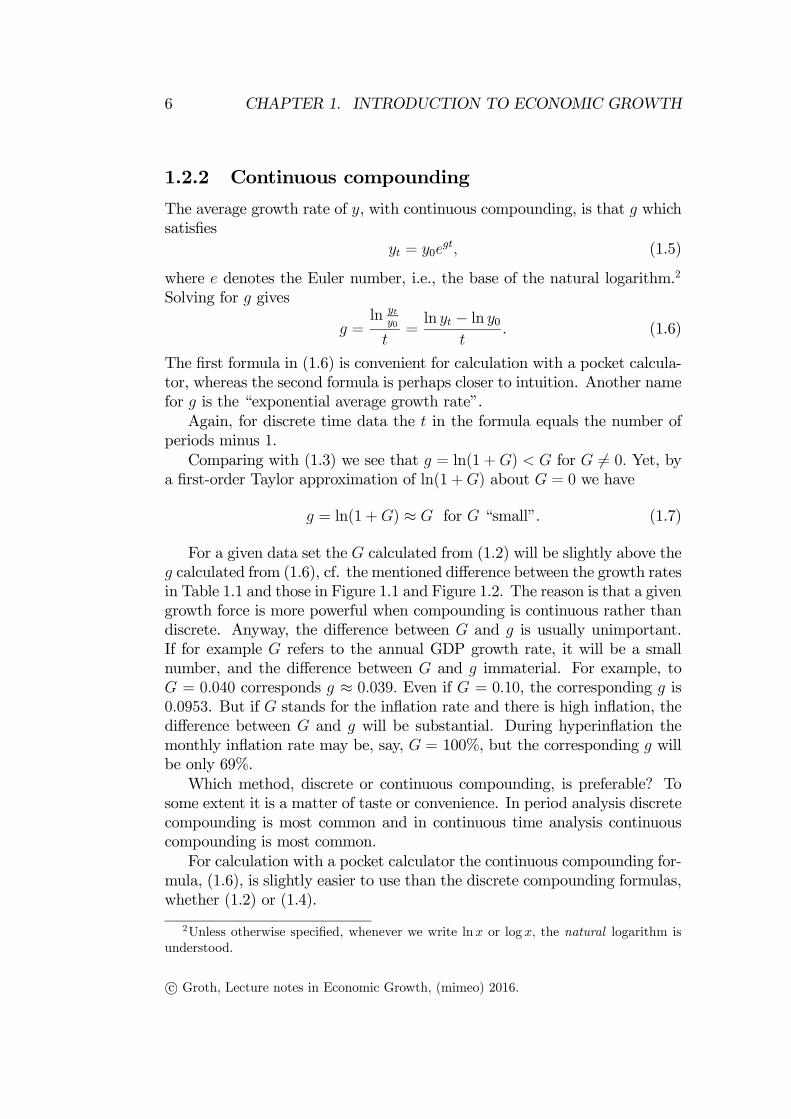
1.2.2 Continuous compounding
The average growth rate of , with continuous compounding, is that which
satisfies
= 0 (1.5)
where denotes the Euler number, i.e., the base of the natural logarithm.2
Solving for gives
=ln
0
=ln − ln 0
(1.6)
The first formula in (1.6) is convenient for calculation with a pocket calcula-
tor, whereas the second formula is perhaps closer to intuition. Another name
for is the “exponential average growth rate”.
Again, for discrete time data the in the formula equals the number of
periods minus 1.
Comparing with (1.3) we see that = ln(1 +) for 6= 0 Yet, bya first-order Taylor approximation of ln(1 +) about = 0 we have
= ln(1 +) ≈ for “small”. (1.7)
For a given data set the calculated from (1.2) will be slightly above the
calculated from (1.6), cf. the mentioned difference between the growth rates
in Table 1.1 and those in Figure 1.1 and Figure 1.2. The reason is that a given
growth force is more powerful when compounding is continuous rather than
discrete. Anyway, the difference between and is usually unimportant.
If for example refers to the annual GDP growth rate, it will be a small
number, and the difference between and immaterial. For example, to
= 0040 corresponds ≈ 0039 Even if = 010, the corresponding is
00953. But if stands for the inflation rate and there is high inflation, the
difference between and will be substantial. During hyperinflation the
monthly inflation rate may be, say, = 100%, but the corresponding will
be only 69%.
Which method, discrete or continuous compounding, is preferable? To
some extent it is a matter of taste or convenience. In period analysis discrete
compounding is most common and in continuous time analysis continuous
compounding is most common.
For calculation with a pocket calculator the continuous compounding for-
mula, (1.6), is slightly easier to use than the discrete compounding formulas,
whether (1.2) or (1.4).
2Unless otherwise specified, whenever we write ln or log the natural logarithm is
understood.
c° Groth, Lecture notes in Economic Growth, (mimeo) 2016.
1.3. Some stylized facts of economic growth 7
To avoid too much sensitiveness to the initial and terminal observations,
which may involve measurement error or depend on the state of the business
cycle, one can use an OLS approach to the trend coefficient, in the following
regression:
ln = + +
This is in fact what is done in Fig. 1.1.
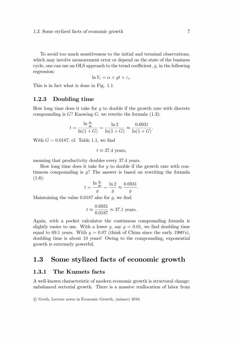
1.2.3 Doubling time
How long time does it take for to double if the growth rate with discrete
compounding is ? Knowing we rewrite the formula (1.3):
=ln
0
ln(1 +)=
ln 2
ln(1 +)≈ 06931
ln(1 +)
With = 00187 cf. Table 1.1, we find
≈ 374 years,meaning that productivity doubles every 374 years.
How long time does it take for to double if the growth rate with con-
tinuous compounding is ? The answer is based on rewriting the formula
(1.6):
=ln
0
=ln 2
≈ 06931
Maintaining the value 00187 also for we find
≈ 0693100187
≈ 371 years.
Again, with a pocket calculator the continuous compounding formula is
slightly easier to use. With a lower say = 001 we find doubling time
equal to 691 years. With = 007 (think of China since the early 1980’s),
doubling time is about 10 years! Owing to the compounding, exponential
growth is extremely powerful.
1.3 Some stylized facts of economic growth
1.3.1 The Kuznets facts
A well-known characteristic of modern economic growth is structural change:
unbalanced sectorial growth. There is a massive reallocation of labor from
c° Groth, Lecture notes in Economic Growth, (mimeo) 2016.
8 CHAPTER 1. INTRODUCTION TO ECONOMIC GROWTH
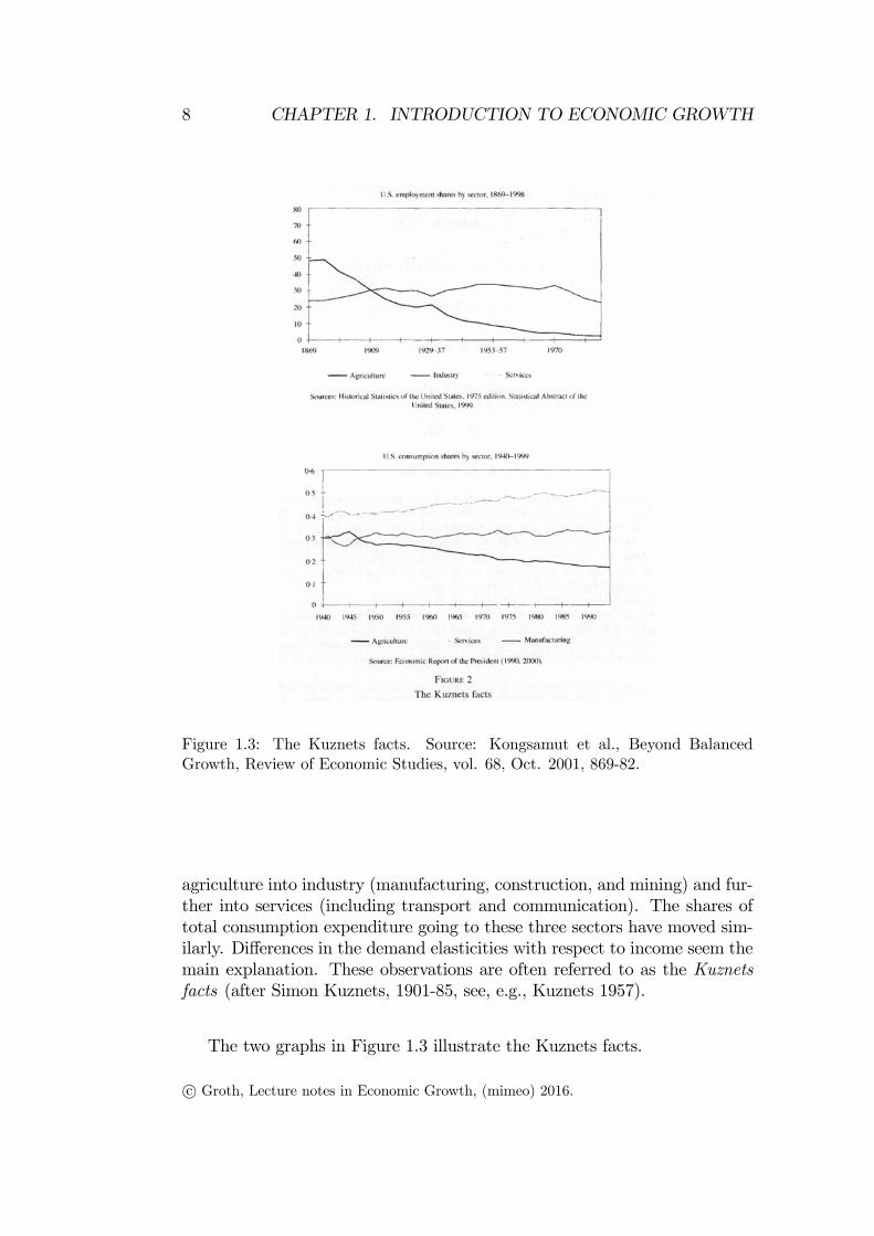
Figure 1.3: The Kuznets facts. Source: Kongsamut et al., Beyond Balanced
Growth, Review of Economic Studies, vol. 68, Oct. 2001, 869-82.
agriculture into industry (manufacturing, construction, and mining) and fur-
ther into services (including transport and communication). The shares of
total consumption expenditure going to these three sectors have moved sim-
ilarly. Differences in the demand elasticities with respect to income seem the
main explanation. These observations are often referred to as the Kuznets
facts (after Simon Kuznets, 1901-85, see, e.g., Kuznets 1957).
The two graphs in Figure 1.3 illustrate the Kuznets facts.
c° Groth, Lecture notes in Economic Growth, (mimeo) 2016.
1.3. Some stylized facts of economic growth 9
1.3.2 Kaldor’s stylized facts
Surprisingly, in spite of the Kuznets facts, the evolution at the aggregate level
in developed countries is by many economists seen as roughly described by
what is called Kaldor’s “stylized facts” (after the Hungarian-British econo-
mist Nicholas Kaldor, 1908-1986, see, e.g., Kaldor 1957, 1961)3:
1. Real output per man-hour grows at a more or less constant rate
over fairly long periods of time. (Of course, there are short-run fluctuations
superposed around this trend.)
2. The stock of physical capital per man-hour grows at a more or less
constant rate over fairly long periods of time.
3. The ratio of output to capital shows no systematic trend.
4. The rate of return to capital shows no systematic trend.
5. The income shares of labor and capital (in the national account-
ing sense, i.e., including land and other natural resources), respectively, are
nearly constant.
6. The growth rate of output per man-hour differs substantially across
countries.
These claimed regularities do certainly not fit all developed countries
equally well. Although Solow’s growth model (Solow, 1956) can be seen as the
first successful attempt at building a model consistent with Kaldor’s “stylized
facts”, Solow once remarked about them: “There is no doubt that they are
stylized, though it is possible to question whether they are facts” (Solow,
1970). Yet, for instance the study by Attfield and Temple (2010) of US and
UK data since the Second World War concludes with support for Kaldor’s
“facts”. Recently, several empiricists4 have questioned “fact” 5, however,
referring to the inadequacy of the methods which standard national income
accounting applies to separate the income of entrepreneurs, sole proprietors,
and unincorporated businesses into labor and capital income. It is claimed
that these methods obscure a tendency in recent decades of the labor income
share to fall.
The sixth Kaldor fact is, of course, generally accepted as a well docu-
mented observation (a nice summary is contained in Pritchett, 1997).
Kaldor also proposed hypotheses about the links between growth in the
different sectors (see, e.g., Kaldor 1967):
a. Productivity growth in the manufacturing and construction sec-
tors is enhanced by output growth in these sectors (this is also known as
Verdoorn’s Law). Increasing returns to scale and learning by doing are the
main factors behind this.
3Kaldor presented his six regularities as “a stylised view of the facts”.4E.g., Gollin (2002), Elsby et al. (2013), and Karabarbounis and Neiman (2014).
c° Groth, Lecture notes in Economic Growth, (mimeo) 2016.
10 CHAPTER 1. INTRODUCTION TO ECONOMIC GROWTH
b. Productivity growth in agriculture and services is enhanced by out-
put growth in the manufacturing and construction sectors.
Kongsamut et al. (2001) and Foellmi and Zweimüller (2008) offer theoret-
ical explanations of why the Kuznets facts and the Kaldor facts can coexist.
1.4 Concepts of income convergence
The two most popular across-country income convergence concepts are “
convergence” and “ convergence”.
1.4.1 convergence vs. convergence
Definition 1 We say that convergence occurs for a given selection of coun-
tries if there is a tendency for the poor (those with low income per capita or
low output per worker) to subsequently grow faster than the rich.
By “grow faster” is meant that the growth rate of per capita income (or
per worker output) is systematically higher.
In many contexts, a more appropriate convergence concept is the follow-
ing:
Definition 2 We say that convergence, with respect to a given measure of
dispersion, occurs for a given collection of countries if this measure of disper-
sion, applied to income per capita or output per worker across the countries,
declines systematically over time. On the other hand, divergence occurs, if
the dispersion increases systematically over time.
The reason that convergence must be considered the more appropri-
ate concept is the following. In the end, it is the question of increasing
or decreasing dispersion across countries that we are interested in. From a
superficial point of view one might think that convergence implies decreas-
ing dispersion and vice versa, so that convergence and convergence are
more or less equivalent concepts. But since the world is not deterministic,
but stochastic, this is not true. Indeed, convergence is only a necessary,
not a sufficient condition for convergence. This is because over time some
reshuffling among the countries is always taking place, and this implies that
there will always be some extreme countries (those initially far away from
the mean) that move closer to the mean, thus creating a negative correla-
tion between initial level and subsequent growth, in spite of equally many
c° Groth, Lecture notes in Economic Growth, (mimeo) 2016.
1.4. Concepts of income convergence 11
countries moving from a middle position toward one of the extremes.5 In
this way convergence may be observed at the same time as there is no
convergence; the mere presence of random measurement errors implies a bias
in this direction because a growth rate depends negatively on the initial mea-
surement and positively on the later measurement. In fact, convergence
may be consistent with divergence (for a formal proof of this claim, see
Barro and Sala-i-Martin, 2004, pp. 50-51 and 462 ff.; see also Valdés, 1999,
p. 49-50, and Romer, 2001, p. 32-34).
Hence, it is wrong to conclude from convergence (poor countries tend
to grow faster than rich ones) to convergence (reduced dispersion of per
capita income) without any further investigation. The mistake is called “re-
gression towards the mean” or “Galton’s fallacy”. Francis Galton was an
anthropologist (and a cousin of Darwin), who in the late nineteenth century
observed that tall fathers tended to have not as tall sons and small fathers
tended to have taller sons. From this he falsely concluded that there was
a tendency to averaging out of the differences in height in the population.
Indeed, being a true aristocrat, Galton found this tendency pitiable. But
since his conclusion was mistaken, he did not really have to worry.
Since convergence comes closer to what we are ultimately looking for,
from now, when we speak of just “income convergence”, convergence is
understood.
In the above definitions of convergence and convergence, respectively,
we were vague as to what kind of selection of countries is considered. In
principle we would like it to be a representative sample of the “population”
of countries that we are interested in. The population could be all countries
in the world. Or it could be the countries that a century ago had obtained a
certain level of development.
One should be aware that historical GDP data are constructed retrospec-
tively. Long time series data have only been constructed for those countries
that became relatively rich during the after-WWII period. Thus, if we as our
sample select the countries for which long data series exist, what is known as
selection bias is involved which generates a spurious convergence. A country
which was poor a century ago will only appear in the sample if it grew rapidly
over the next 100 years. A country which was relatively rich a century ago
will appear in the sample unconditionally. This selection bias problem was
5As an intuitive analogy, think of the ordinal rankings of the sports teams in a league.
The dispersion of rankings is constant by definition. Yet, no doubt there will allways be
some tendency for weak teams to rebound toward the mean and of champions to revert
to mediocrity. (This example is taken from the first edition of Barro and Sala-i-Martin,
Economic Growth, 1995; I do not know why, but the example was deleted in the second
edition from 2004.)
c° Groth, Lecture notes in Economic Growth, (mimeo) 2016.
12 CHAPTER 1. INTRODUCTION TO ECONOMIC GROWTH
pointed out by DeLong (1988) in a criticism of widespread false interpreta-
tions of Maddison’s long data series (Maddison 1982).
1.4.2 Measures of dispersion
Our next problem is: what measure of dispersion is to be used as a useful
descriptive statistics for convergence? Here there are different possibilities.
To be precise about this we need some notation. Let
≡
and
≡
where = real GDP, = employment, and = population. If the focus
is on living standards, is the relevant variable.6 But if the focus is on
(labor) productivity, it is that is relevant. Since most growth models
focus on rather than let os take as our example.
One might think that the standard deviation of could be a relevant
measure of dispersion when discussing whether convergence is present or
not. The standard deviation of across countries in a given year is
≡vuut1
X=1
( − )2 (1.8)
where
≡P
(1.9)
i.e., is the average output per worker. However, if this measure were used,
it would be hard to find any group of countries for which there is income
convergence. This is because tends to grow over time for most countries,
and then there is an inherent tendency for the variance also to grow; hence
also the square root of the variance, tends to grow. Indeed, suppose that
for all countries, is doubled from time 1 to time 2 Then, automatically,
is also doubled. But hardly anyone would interpret this as an increase in
the income inequality across the countries.
Hence, it is more adequate to look at the standard deviation of relative
income levels:
≡s1
X
(
− 1)2 (1.10)
6Or perhaps better, where ≡ ≡ − − Here, denotes net
interest payments on foreign debt and denotes net labor income of foreign workers in
the country.
c° Groth, Lecture notes in Economic Growth, (mimeo) 2016.
1.4. Concepts of income convergence 13
This measure is the same as what is called the coefficient of variation,
usually defined as
≡
(1.11)
that is, the standard deviation of standardized by the mean. That the two
measures are identical can be seen in this way:
≡
q1
P( − )2
=
s1
X
( −
)2 =
s1
X
(
− 1)2 ≡
The point is that the coefficient of variation is “scale free”, which the standard
deviation itself is not.
Instead of the coefficient of variation, another scale free measure is often
used, namely the standard deviation of ln , i.e.,
ln ≡s1
X
(ln − ln ∗)2 (1.12)
where
ln ∗ ≡P
ln
(1.13)
Note that ∗ is the geometric average, i.e., ∗ ≡ √12 · · · Now, by a
first-order Taylor approximation of ln around = , we have
ln ≈ ln + 1( − )
Hence, as a very rough approximation we have ln ≈ = though
this approximation can be quite poor (cf. Dalgaard and Vastrup, 2001).
It may be possible, however, to defend the use of ln in its own right to
the extent that tends to be approximately lognormally distributed across
countries.
Yet another possible measure of income dispersion across countries is the
Gini index (see for example Cowell, 1995).
1.4.3 Weighting by size of population
Another important issue is whether the applied dispersion measure is based
on a weighting of the countries by size of population. For the world as a
whole, when no weighting by size of population is used, then there is a slight
tendency to income divergence according to the ln criterion (Acemoglu,
c° Groth, Lecture notes in Economic Growth, (mimeo) 2016.
14 CHAPTER 1. INTRODUCTION TO ECONOMIC GROWTH
2009, p. 4), where is per capita income (≡ ). As seen by Fig. 4 below,
this tendency is not so clear according to the criterion. Anyway, when
there is weighting by size of population, then in the last twenty years there
has been a tendency to income convergence at the global level (Sala-i-Martin
2006; Acemoglu, 2009, p. 6). With weighting by size of population (1.12) is
modified to
ln ≡sX
(ln − ln ∗)2
where
=
and ln ∗ ≡
X
ln
1.4.4 Unconditional vs. conditional convergence
Yet another distinction in the study of income convergence is that between
unconditional (or absolute) and conditional convergence. We say that a
large heterogeneous group of countries (say the countries in the world) show
unconditional income convergence if income convergence occurs for the whole
group without conditioning on specific characteristics of the countries. If
income convergence occurs only for a subgroup of the countries, namely those
countries that in advance share the same “structural characteristics”, then
we say there is conditional income convergence. As noted earlier, when we
speak of just income “convergence”, income “ convergence” is understood.
If in a given context there might be doubt, one should of course be explicit
and speak of unconditional or conditional convergence. Similarly, if the
focus for some reason is on convergence, we should distinguish between
unconditional and conditional convergence.
What the precise meaning of “structural characteristics” is, will depend
on what model of the countries the researcher has in mind. According to
the Solow model, a set of relevant “structural characteristics” are: the aggre-
gate production function, the initial level of technology, the rate of technical
progress, the capital depreciation rate, the saving rate, and the population
growth rate. But the Solow model, as well as its extension with human cap-
ital (Mankiw et al., 1992), is a model of a closed economy with exogenous
technical progress. The model deals with “within-country” convergence in
the sense that the model predicts that a closed economy being initially be-
low or above its steady state path, will over time converge towards its steady
state path. It is far from obvious that this kind of model is a good model
of cross-country convergence in a globalized world where capital mobility
and to some extent also labor mobility are important and some countries are
c° Groth, Lecture notes in Economic Growth, (mimeo) 2016.
1.4. Concepts of income convergence 15
0
3000
6000
9000
12000
15000
18000
21000
1950 1960 1970 1980 1990 2000
Dispersion of GDP per capita
Dispersion of GDP per worker
Dispersion
Year
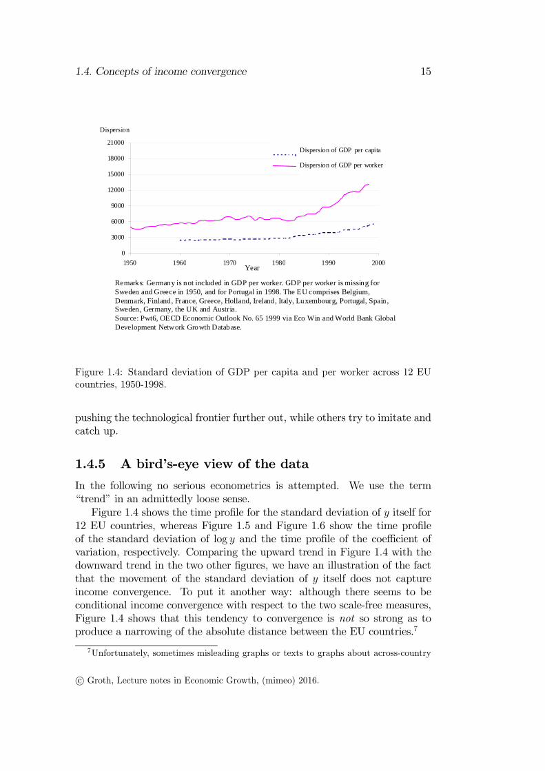
Remarks: Germany is not included in GDP per worker. GDP per worker is missing for Sweden and Greece in 1950, and for Portugal in 1998. The EU comprises Belgium, Denmark, Finland, France, Greece, Holland, Ireland, Italy, Luxembourg, Portugal, Spain, Sweden, Germany, the UK and Austria. Source: Pwt6, OECD Economic Outlook No. 65 1999 via Eco Win and World Bank Global Development Network Growth Database.
Figure 1.4: Standard deviation of GDP per capita and per worker across 12 EU
countries, 1950-1998.
pushing the technological frontier further out, while others try to imitate and
catch up.
1.4.5 A bird’s-eye view of the data
In the following no serious econometrics is attempted. We use the term
“trend” in an admittedly loose sense.
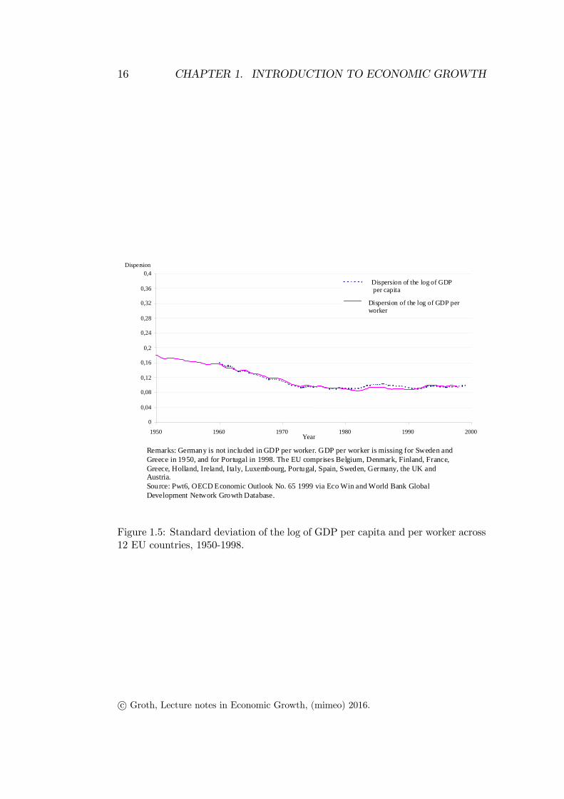
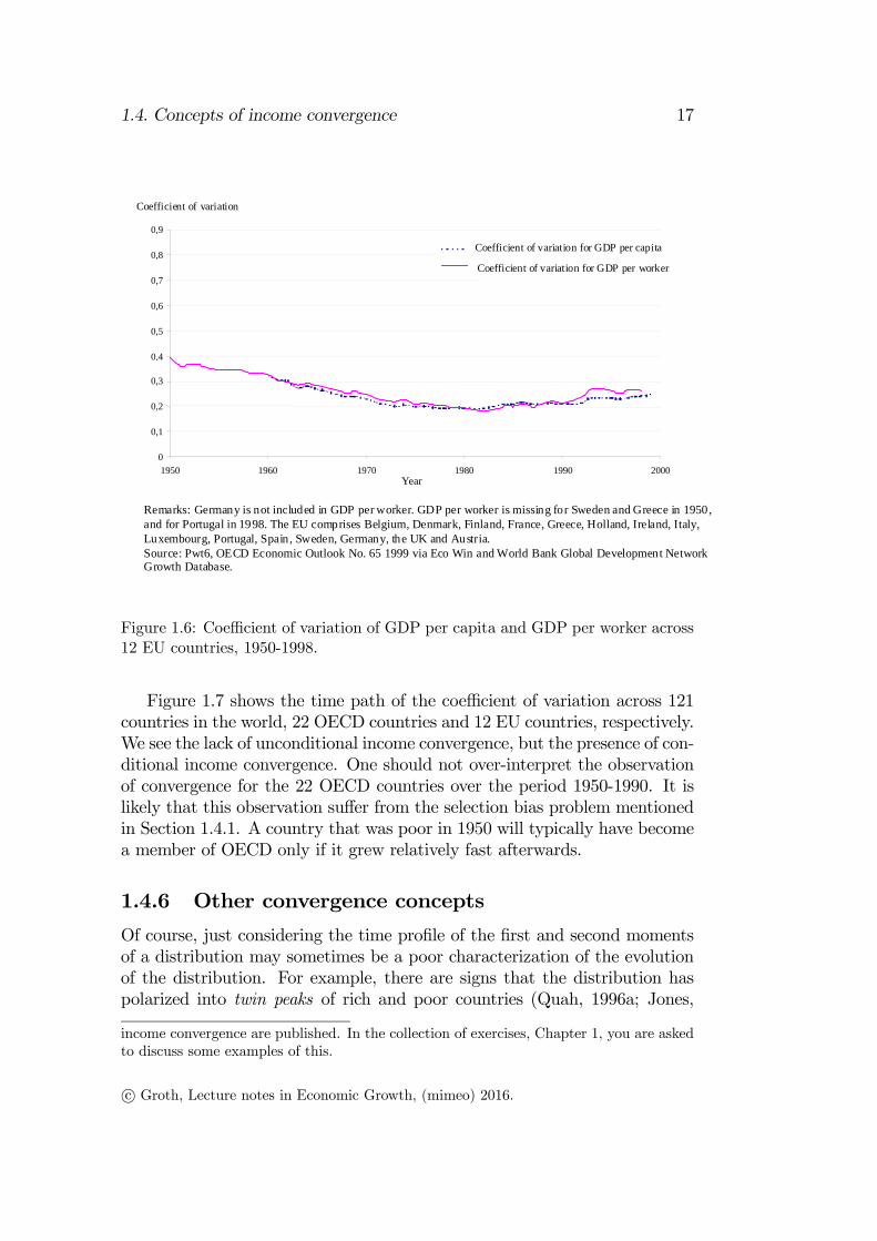
Figure 1.4 shows the time profile for the standard deviation of itself for
12 EU countries, whereas Figure 1.5 and Figure 1.6 show the time profile
of the standard deviation of log and the time profile of the coefficient of
variation, respectively. Comparing the upward trend in Figure 1.4 with the
downward trend in the two other figures, we have an illustration of the fact
that the movement of the standard deviation of itself does not capture
income convergence. To put it another way: although there seems to be
conditional income convergence with respect to the two scale-free measures,
Figure 1.4 shows that this tendency to convergence is not so strong as to
produce a narrowing of the absolute distance between the EU countries.7
7Unfortunately, sometimes misleading graphs or texts to graphs about across-country
c° Groth, Lecture notes in Economic Growth, (mimeo) 2016.
16 CHAPTER 1. INTRODUCTION TO ECONOMIC GROWTH
0
0,04
0,08
0,12
0,16
0,2
0,24
0,28
0,32
0,36
0,4
1950 1960 1970 1980 1990 2000
Dispersion
Dispersion of the log of GDP per capita
Dispersion of the log of GDP per worker
Year
Remarks: Germany is not included in GDP per worker. GDP per worker is missing for Sweden and Greece in 1950, and for Portugal in 1998. The EU comprises Belgium, Denmark, Finland, France, Greece, Holland, Ireland, Italy, Luxembourg, Portugal, Spain, Sweden, Germany, the UK and Austria. Source: Pwt6, OECD Economic Outlook No. 65 1999 via Eco Win and World Bank Global Development Network Growth Database.
Figure 1.5: Standard deviation of the log of GDP per capita and per worker across
12 EU countries, 1950-1998.
c° Groth, Lecture notes in Economic Growth, (mimeo) 2016.
1.4. Concepts of income convergence 17
0
0,1
0,2
0,3
0,4
0,5
0,6
0,7
0,8
0,9
1950 1960 1970 1980 1990 2000
Coefficient of variation
Coefficient of variation for GDP per capita
Coefficient of variation for GDP per worker
Year
Remarks: Germany is not included in GDP per worker. GDP per worker is missing for Sweden and Greece in 1950, and for Portugal in 1998. The EU comprises Belgium, Denmark, Finland, France, Greece, Holland, Ireland, Italy, Luxembourg, Portugal, Spain, Sweden, Germany, the UK and Austria. Source: Pwt6, OECD Economic Outlook No. 65 1999 via Eco Win and World Bank Global Development Network Growth Database.
Figure 1.6: Coefficient of variation of GDP per capita and GDP per worker across
12 EU countries, 1950-1998.
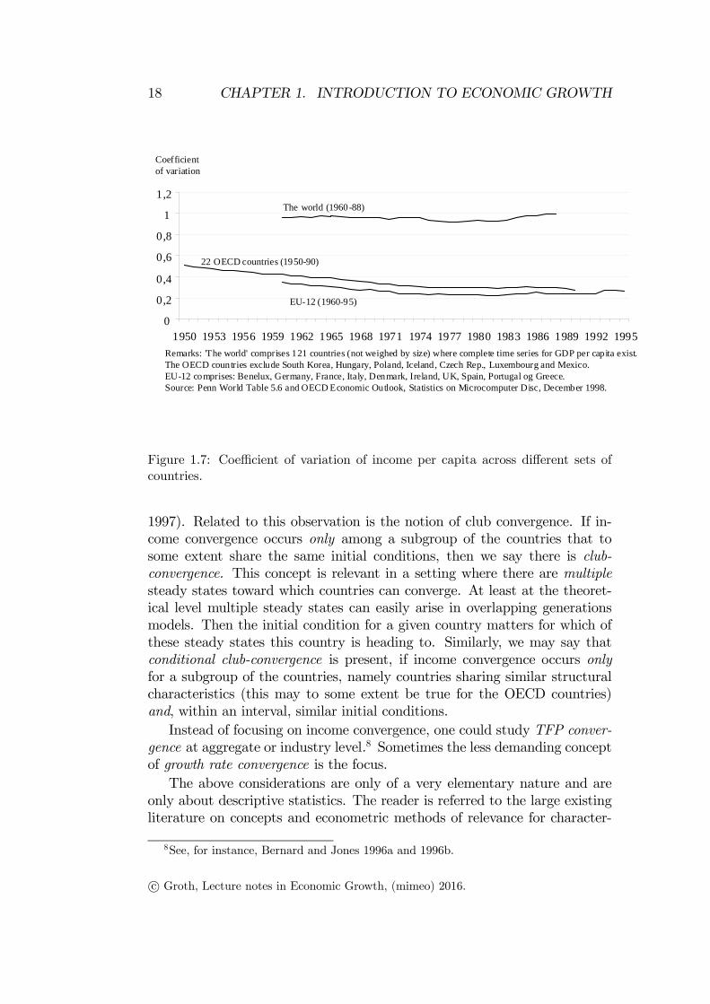
Figure 1.7 shows the time path of the coefficient of variation across 121
countries in the world, 22 OECD countries and 12 EU countries, respectively.
We see the lack of unconditional income convergence, but the presence of con-
ditional income convergence. One should not over-interpret the observation
of convergence for the 22 OECD countries over the period 1950-1990. It is
likely that this observation suffer from the selection bias problem mentioned
in Section 1.4.1. A country that was poor in 1950 will typically have become
a member of OECD only if it grew relatively fast afterwards.
1.4.6 Other convergence concepts
Of course, just considering the time profile of the first and second moments
of a distribution may sometimes be a poor characterization of the evolution
of the distribution. For example, there are signs that the distribution has
polarized into twin peaks of rich and poor countries (Quah, 1996a; Jones,
income convergence are published. In the collection of exercises, Chapter 1, you are asked
to discuss some examples of this.
c° Groth, Lecture notes in Economic Growth, (mimeo) 2016.
18 CHAPTER 1. INTRODUCTION TO ECONOMIC GROWTH
0
0,2
0,4
0,6
0,8
1
1,2
1950 1953 1956 1959 1962 1965 1968 1971 1974 1977 1980 1983 1986 1989 1992 1995
Coefficient of variation
22 OECD countries (1950-90)
EU-12 (1960-95)
The world (1960-88)
Remarks: 'The world' comprises 121 countries (not weighed by size) where complete time series for GDP per capita exist. The OECD countries exclude South Korea, Hungary, Poland, Iceland, Czech Rep., Luxembourg and Mexico. EU-12 comprises: Benelux, Germany, France, Italy, Denmark, Ireland, UK, Spain, Portugal og Greece. Source: Penn World Table 5.6 and OECD Economic Outlook, Statistics on Microcomputer Disc, December 1998.
Coefficient of variation
Figure 1.7: Coefficient of variation of income per capita across different sets of
countries.
1997). Related to this observation is the notion of club convergence. If in-
come convergence occurs only among a subgroup of the countries that to
some extent share the same initial conditions, then we say there is club-
convergence. This concept is relevant in a setting where there are multiple
steady states toward which countries can converge. At least at the theoret-
ical level multiple steady states can easily arise in overlapping generations
models. Then the initial condition for a given country matters for which of
these steady states this country is heading to. Similarly, we may say that
conditional club-convergence is present, if income convergence occurs only
for a subgroup of the countries, namely countries sharing similar structural
characteristics (this may to some extent be true for the OECD countries)
and, within an interval, similar initial conditions.
Instead of focusing on income convergence, one could study TFP conver-
gence at aggregate or industry level.8 Sometimes the less demanding concept
of growth rate convergence is the focus.
The above considerations are only of a very elementary nature and are
only about descriptive statistics. The reader is referred to the large existing
literature on concepts and econometric methods of relevance for character-
8See, for instance, Bernard and Jones 1996a and 1996b.
c° Groth, Lecture notes in Economic Growth, (mimeo) 2016.
1.5. Literature 19
izing the evolution of world income distribution (see Quah, 1996b, 1996c,
1997, and for a survey, see Islam 2003).
1.5 Literature
Acemoglu, D., 2009, Introduction to Modern Economic Growth, Princeton
University Press: Oxford.
Acemoglu, D., and V. Guerrieri, 2008, Capital deepening and nonbalanced
economic growth, J. Political Economy, vol. 116 (3), 467- .
Attfield, C., and J.R.W. Temple, 2010, Balanced growth and the great
ratios: New evidence for the US and UK, Journal of Macroeconomics,
vol. 32, 937-956.
Barro, R. J., and X. Sala-i-Martin, 1995, Economic Growth, MIT Press,
New York. Second edition, 2004.
Bernard, A.B., and C.I. Jones, 1996a, ..., Economic Journal.
- , 1996b, Comparing Apples to Oranges: Productivity Convergence and
Measurement Across Industries and Countries, American Economic
Review, vol. 86 (5), 1216-1238.
Cowell, Frank A., 1995, Measuring Inequality. 2. ed., London.
Dalgaard, C.-J., and J. Vastrup, 2001, On the measurement of -convergence,
Economics letters, vol. 70, 283-87.
Dansk økonomi. Efterår 2001, (Det økonomiske Råds formandskab) Kbh.
2001.
Deininger, K., and L. Squire, 1996, A new data set measuring income in-
equality, The World Bank Economic Review, 10, 3.
Delong, B., 1988, ... American Economic Review.
Foellmi, R., and J. Zweimüller, 2008, ..., JME, 55, 1317-1328.
Handbook of Economic Growth, vol. 1A and 1B, ed. by S. N. Durlauf and
P. Aghion, Amsterdam 2005.
Handbook of Income Distribution, vol. 1, ed. by A.B. Atkinson and F.
Bourguignon, Amsterdam 2000.
c° Groth, Lecture notes in Economic Growth, (mimeo) 2016.
20 CHAPTER 1. INTRODUCTION TO ECONOMIC GROWTH
Islam, N., 2003, What have we learnt from the convergence debate? Journal
of Economic Surveys 17, 3, 309-62.
Kaldor, N., 1957, A model of economic growth, The Economic Journal, vol.
67, pp. 591-624.
- , 1961, “Capital Accumulation and Economic Growth”. In: F. Lutz, ed.,
Theory of Capital, London: MacMillan.
- , 1967, Strategic Factors in Economic Development, New York State School
of Industrial and Labor Relations, Cornell University.
Kongsamut, P., S. Rebelo, and D. Xie, 2001, Beyond Balanced Growth,
Review of Economic Studies, vol. 68, 869-882.
Kuznets, S., 1957, Quantitative aspects of economic growth of nations: II,
Economic Development and Cultural Change, Supplement to vol. 5,
3-111.
Maddison, A., 1982,
Maddison, A., Contours ...., Cambridge University Press.
Mankiw, N.G., D. Romer, and D.N. Weil, 1992,
Pritchett, L., 1997, Divergence — big time, Journal of Economic Perspec-
tives, vol. 11, no. 3.
Quah, D., 1996a, Twin peaks ..., Economic Journal, vol. 106, 1045-1055.
-, 1996b, Empirics for growth and convergence, European Economic Review,
vol. 40 (6).
-, 1996c, Convergence empirics ..., J. of Ec. Growth, vol. 1 (1).
-, 1997, Searching for prosperity: A comment, Carnegie-Rochester Confer-
ende Series on Public Policy, vol. 55, 305-319.
Romer, D., 2012, Advanced Macroeconomics, 4th ed., McGraw-Hill: New
York.
Sala-i-Martin, X., 2006, The World Distribution of Income, Quarterly Jour-
nal of Economics 121, No. 2.
Sen, A., ...
c° Groth, Lecture notes in Economic Growth, (mimeo) 2016.
1.5. Literature 21
Solow, R.M., 1970, Growth theory. An exposition, Clarendon Press: Oxford.
Second enlarged edition, 2000.
Valdés, B., 1999, Economic Growth. Theory, Empirics, and Policy, Edward
Elgar.
Onmeasurement problems, see: http://www.worldbank.org/poverty/inequal/methods/index.htm
c° Groth, Lecture notes in Economic Growth, (mimeo) 2016.
22 CHAPTER 1. INTRODUCTION TO ECONOMIC GROWTH
c° Groth, Lecture notes in Economic Growth, (mimeo) 2016.
Chapter 2
Review of technology andfactor shares of income
The aim of this chapter is, first, to introduce the terminology concerningfirms’technology and technological change used in the lectures and exercisesof this course. At a few points I deviate somewhat from definitions in Ace-moglu’s book. Section 1.3 can be used as a formula manual for the case ofCRS.Second, the chapter contains a brief discussion of the notions of a repre-
sentative firm and an aggregate production function. The distinction betweenlong-run versus short-run production functions is also commented on. Thelast sections introduce the concept of elasticity of substitution between cap-ital and labour and its role for the direction of movement over time of theincome shares of capital and labor under perfect competition.Regarding the distinction between discrete and continuous time analysis,
most of the definitions contained in this chapter are applicable to both.
2.1 The production technology
Consider a two-factor production function given by
Y = F (K,L), (2.1)
where Y is output (value added) per time unit, K is capital input per timeunit, and L is labor input per time unit (K ≥ 0, L ≥ 0). We may think of(2.1) as describing the output of a firm, a sector, or the economy as a whole.It is in any case a very simplified description, ignoring the heterogeneity ofoutput, capital, and labor. Yet, for many macroeconomic questions it maybe a useful first approach. Note that in (2.1) not only Y but also K and L
23
24CHAPTER 2. REVIEW OF TECHNOLOGY AND
FACTOR SHARES OF INCOME
represent flows, that is, quantities per unit of time. If the time unit is oneyear, we think of K as measured in machine hours per year. Similarly, wethink of L as measured in labor hours per year. Unless otherwise specified, itis understood that the rate of utilization of the production factors is constantover time and normalized to one for each production factor. As explainedin Chapter 1, we can then use the same symbol, K, for the flow of capitalservices as for the stock of capital. Similarly with L.
2.1.1 A neoclassical production function
By definition, K and L are non-negative. It is generally understood that aproduction function, Y = F (K,L), is continuous and that F (0, 0) = 0 (no in-put, no output). Sometimes, when specific functional forms are used to repre-sent a production function, that function may not be defined at points whereK = 0 or L = 0 or both. In such a case we adopt the convention that the do-main of the function is understood extended to include such boundary pointswhenever it is possible to assign function values to them such that continuityis maintained. For instance the function F (K,L) = αL + βKL/(K + L),where α > 0 and β > 0, is not defined at (K,L) = (0, 0). But by assigningthe function value 0 to the point (0, 0), we maintain both continuity and the“no input, no output”property.We call the production function neoclassical if for all (K,L), with K > 0
and L > 0, the following additional conditions are satisfied:
(a) F (K,L) has continuous first- and second-order partial derivatives sat-isfying:
FK > 0, FL > 0, (2.2)
FKK < 0, FLL < 0. (2.3)
(b) F (K,L) is strictly quasiconcave (i.e., the level curves, also called iso-quants, are strictly convex to the origin).
In words: (a) says that a neoclassical production function has continuoussubstitution possibilities between K and L and the marginal productivitiesare positive, but diminishing in own factor. Thus, for a given number of ma-chines, adding one more unit of labor, adds to output, but less so, the higheris already the labor input. And (b) says that every isoquant, F (K,L) = Y ,has a strictly convex form qualitatively similar to that shown in Figure 2.1.1
1For any fixed Y ≥ 0, the associated isoquant is the level set{(K,L) ∈ R+| F (K,L) = Y
}.
c© Groth, Lecture notes in Economic Growth, (mimeo) 2016.
2.1. The production technology 25
When we speak of for example FL as the marginal productivity of labor, itis because the “pure” partial derivative, ∂Y/∂L = FL, has the denomina-tion of a productivity (output units/yr)/(man-yrs/yr). It is quite common,however, to refer to FL as the marginal product of labor. Then a unit mar-ginal increase in the labor input is understood: ∆Y ≈ (∂Y/∂L)∆L = ∂Y/∂Lwhen ∆L = 1. Similarly, FK can be interpreted as the marginal productiv-ity of capital or as the marginal product of capital. In the latter case it isunderstood that ∆K = 1, so that ∆Y ≈ (∂Y/∂K)∆K = ∂Y/∂K.
The definition of a neoclassical production function can be extended tothe case of n inputs. Let the input quantities be X1, X2, . . . , Xn and considera production function Y = F (X1, X2, . . . , Xn). Then F is called neoclassical ifall the marginal productivities are positive, but diminishing, and F is strictlyquasiconcave (i.e., the upper contour sets are strictly convex, cf. AppendixA).Returning to the two-factor case, since F (K,L) presumably depends on
the level of technical knowledge and this level depends on time, t, we mightwant to replace (2.1) by
Yt = F t(Kt, Lt), (2.4)
where the superscript on F indicates that the production function may shiftover time, due to changes in technology. We then say that F t(·) is a neoclas-sical production function if it satisfies the conditions (a) and (b) for all pairs(Kt, Lt). Technological progress can then be said to occur when, for Kt andLt held constant, output increases with t.For convenience, to begin with we skip the explicit reference to time and
level of technology.
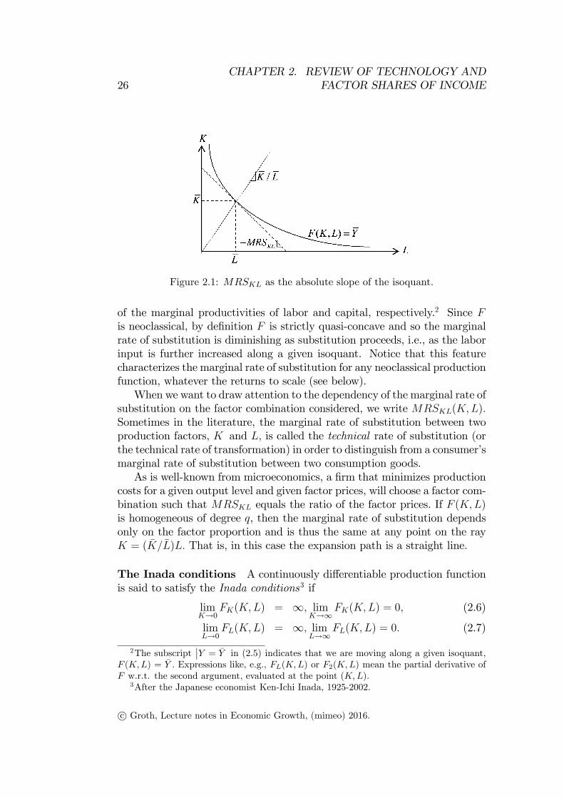
The marginal rate of substitution Given a neoclassical productionfunction F, we consider the isoquant defined by F (K,L) = Y , where Yis a positive constant. The marginal rate of substitution, MRSKL, of K forL at the point (K,L) is defined as the absolute slope of the isoquant at thatpoint, cf. Figure 2.1. The equation F (K,L) = Y defines K as an implicitfunction of L. By implicit differentiation we find FK(K,L)dK/dL +FL(K,L)= 0, from which follows
MRSKL ≡ −dK
dL |Y=Y=FL(K,L)
FK(K,L)> 0. (2.5)
That is, MRSKL measures the amount of K that can be saved (approxi-mately) by applying an extra unit of labor. In turn, this equals the ratio
c© Groth, Lecture notes in Economic Growth, (mimeo) 2016.
26CHAPTER 2. REVIEW OF TECHNOLOGY AND
FACTOR SHARES OF INCOME
Figure 2.1: MRSKL as the absolute slope of the isoquant.
of the marginal productivities of labor and capital, respectively.2 Since Fis neoclassical, by definition F is strictly quasi-concave and so the marginalrate of substitution is diminishing as substitution proceeds, i.e., as the laborinput is further increased along a given isoquant. Notice that this featurecharacterizes the marginal rate of substitution for any neoclassical productionfunction, whatever the returns to scale (see below).When we want to draw attention to the dependency of the marginal rate of
substitution on the factor combination considered, we write MRSKL(K,L).Sometimes in the literature, the marginal rate of substitution between twoproduction factors, K and L, is called the technical rate of substitution (orthe technical rate of transformation) in order to distinguish from a consumer’smarginal rate of substitution between two consumption goods.As is well-known from microeconomics, a firm that minimizes production
costs for a given output level and given factor prices, will choose a factor com-bination such that MRSKL equals the ratio of the factor prices. If F (K,L)is homogeneous of degree q, then the marginal rate of substitution dependsonly on the factor proportion and is thus the same at any point on the rayK = (K/L)L. That is, in this case the expansion path is a straight line.
The Inada conditions A continuously differentiable production functionis said to satisfy the Inada conditions3 if
limK→0
FK(K,L) = ∞, limK→∞
FK(K,L) = 0, (2.6)
limL→0
FL(K,L) = ∞, limL→∞
FL(K,L) = 0. (2.7)
2The subscript∣∣Y = Y in (2.5) indicates that we are moving along a given isoquant,
F (K,L) = Y . Expressions like, e.g., FL(K,L) or F2(K,L) mean the partial derivative ofF w.r.t. the second argument, evaluated at the point (K,L).
3After the Japanese economist Ken-Ichi Inada, 1925-2002.
c© Groth, Lecture notes in Economic Growth, (mimeo) 2016.
2.1. The production technology 27
In this case, the marginal productivity of either production factor has noupper bound when the input of the factor becomes infinitely small. And themarginal productivity is gradually vanishing when the input of the factorincreases without bound. Actually, (2.6) and (2.7) express four conditions,which it is preferable to consider separately and label one by one. In (2.6) wehave two Inada conditions for MPK (the marginal productivity of capital),the first being a lower, the second an upper Inada condition for MPK. Andin (2.7) we have two Inada conditions for MPL (the marginal productivityof labor), the first being a lower, the second an upper Inada condition forMPL. In the literature, when a sentence like “the Inada conditions areassumed”appears, it is sometimes not made clear which, and how many, ofthe four are meant. Unless it is evident from the context, it is better to beexplicit about what is meant.The definition of a neoclassical production function we gave above is quite
common in macroeconomic journal articles and convenient because of itsflexibility. There are textbooks that define a neoclassical production functionmore narrowly by including the Inada conditions as a requirement for callingthe production function neoclassical. In contrast, in this course, when in agiven context we need one or another Inada condition, we state it explicitlyas an additional assumption.
2.1.2 Returns to scale
If all the inputs are multiplied by some factor, is output then multiplied bythe same factor? There may be different answers to this question, dependingon circumstances. We consider a production function F (K,L) where K > 0and L > 0. Then F is said to have constant returns to scale (CRS for short)if it is homogeneous of degree one, i.e., if for all (K,L) and all λ > 0,
F (λK, λL) = λF (K,L).
As all inputs are scaled up or down by some factor > 1, output is scaled upor down by the same factor.4 The assumption of CRS is often defended bythe replication argument. Before discussing this argument, lets us define thetwo alternative “pure”cases.The production function F (K,L) is said to have increasing returns to
scale (IRS for short) if, for all (K,L) and all λ > 1,
F (λK, λL) > λF (K,L).
4In their definition of a neoclassical production function some textbooks add constantreturns to scale as a requirement besides (a) and (b). This course follows the alternativeterminology where, if in a given context an assumption of constant returns to scale isneeded, this is stated as an additional assumption.
c© Groth, Lecture notes in Economic Growth, (mimeo) 2016.
28CHAPTER 2. REVIEW OF TECHNOLOGY AND
FACTOR SHARES OF INCOME
That is, IRS is present if, when all inputs are scaled up by some factor >1, output is scaled up by more than this factor. The existence of gains byspecialization and division of labor, synergy effects, etc. sometimes speak insupport of this assumption, at least up to a certain level of production. Theassumption is also called the economies of scale assumption.Another possibility is decreasing returns to scale (DRS). This is said to
occur when for all (K,L) and all λ > 1,
F (λK, λL) < λF (K,L).
That is, DRS is present if, when all inputs are scaled up by some factor,output is scaled up by less than this factor. This assumption is also calledthe diseconomies of scale assumption. The underlying hypothesis may bethat control and coordination problems confine the expansion of size. Or,considering the “replication argument”below, DRS may simply reflect thatbehind the scene there is an additional production factor, for example landor a irreplaceable quality of management, which is tacitly held fixed, whenthe factors of production are varied.
EXAMPLE 1 The production function
Y = AKαLβ, A > 0, 0 < α < 1, 0 < β < 1, (2.8)
where A, α, and β are given parameters, is called a Cobb-Douglas productionfunction. The parameter A depends on the choice of measurement units;for a given such choice it reflects “effi ciency”, also called the “total factorproductivity”. As an exercise the reader may verify that (2.8) satisfies (a) and(b) above and is therefore a neoclassical production function. The functionis homogeneous of degree α + β. If α + β = 1, there are CRS. If α + β < 1,there are DRS, and if α + β > 1, there are IRS. Note that α and β mustbe less than 1 in order not to violate the diminishing marginal productivitycondition. �EXAMPLE 2 The production function
Y = min(AK,BL), A > 0, B > 0, (2.9)
where A and B are given parameters, is called a Leontief production functionor a fixed-coeffi cients production function; A and B are called the technicalcoeffi cients. The function is not neoclassical, since the conditions (a) and (b)are not satisfied. Indeed, with this production function the production fac-tors are not substitutable at all. This case is also known as the case of perfectcomplementarity between the production factors. The interpretation is that
c© Groth, Lecture notes in Economic Growth, (mimeo) 2016.
2.1. The production technology 29
already installed production equipment requires a fixed number of workers tooperate it. The inverse of the parameters A and B indicate the required cap-ital input per unit of output and the required labor input per unit of output,respectively. Extended to many inputs, this type of production function isoften used in multi-sector input-output models (also called Leontief models).In aggregate analysis neoclassical production functions, allowing substitutionbetween capital and labor, are more popular than Leontief functions. Butsometimes the latter are preferred, in particular in short-run analysis withfocus on the use of already installed equipment where the substitution pos-sibilities are limited.5 As (2.9) reads, the function has CRS. A generalizedform of the Leontief function is Y = min(AKγ, BLγ), where γ > 0. Whenγ < 1, there are DRS, and when γ > 1, there are IRS. �
The replication argument The assumption of CRS is widely used inmacroeconomics. The model builder may appeal to the replication argument.This is the argument saying that by doubling all the inputs, we should alwaysbe able to double the output, since we are just “replicating”what we arealready doing. Suppose we want to double the production of cars. We maythen build another factory identical to the one we already have, man it withidentical workers and deploy the same material inputs. Then it is reasonableto assume output is doubled.In this context it is important that the CRS assumption is about tech-
nology in the sense of functions linking outputs to inputs. Limits to theavailability of input resources is an entirely different matter. The fact thatfor example managerial talent may be in limited supply does not preclude thethought experiment that if a firm could double all its inputs, including thenumber of talented managers, then the output level could also be doubled.The replication argument presupposes, first, that all the relevant inputs
are explicit as arguments in the production function; second, that these arechanged equiproportionately. This, however, exhibits the weakness of thereplication argument as a defence for assuming CRS of our present productionfunction, F (·). One could easily make the case that besides capital and labor,also land is a necessary input and should appear as a separate argument.6
If an industrial firm decides to duplicate what it has been doing, it needs apiece of land to build another plant like the first. Then, on the basis of thereplication argument we should in fact expect DRS w.r.t. capital and laboralone. In manufacturing and services, empirically, this and other possible
5Cf. Section 2.4.6We think of “capital” as producible means of production, whereas “land” refers to
non-producible natural resources, including for example building sites.
c© Groth, Lecture notes in Economic Growth, (mimeo) 2016.
30CHAPTER 2. REVIEW OF TECHNOLOGY AND
FACTOR SHARES OF INCOME
sources for departure from CRS may be minor and so many macroeconomistsfeel comfortable enough with assuming CRS w.r.t. K and L alone, at leastas a first approximation. This approximation is, however, less applicable topoor countries, where natural resources may be a quantitatively importantproduction factor.There is a further problem with the replication argument. Strictly speak-
ing, the CRS claim is that by changing all the inputs equiproportionatelyby any positive factor, λ, which does not have to be an integer, the firmshould be able to get output changed by the same factor. Hence, the replica-tion argument requires that indivisibilities are negligible, which is certainlynot always the case. In fact, the replication argument is more an argumentagainst DRS than for CRS in particular. The argument does not rule outIRS due to synergy effects as size is increased.Sometimes the replication line of reasoning is given a more subtle form.
This builds on a useful local measure of returns to scale, named the elasticityof scale.
The elasticity of scale* To allow for indivisibilities and mixed cases (forexample IRS at low levels of production and CRS or DRS at higher levels),we need a local measure of returns to scale. One defines the elasticity ofscale, η(K,L), of F at the point (K,L), where F (K,L) > 0, as
η(K,L) =λ
F (K,L)
dF (λK, λL)
dλ≈ ∆F (λK, λL)/F (K,L)
∆λ/λ, evaluated at λ = 1.
(2.10)So the elasticity of scale at a point (K,L) indicates the (approximate) per-centage increase in output when both inputs are increased by 1 percent. Wesay that
if η(K,L)
> 1, then there are locally IRS,= 1, then there are locally CRS,< 1, then there are locally DRS.
(2.11)
The production function may have the same elasticity of scale everywhere.This is the case if and only if the production function is homogeneous. If Fis homogeneous of degree h, then η(K,L) = h and h is called the elasticityof scale parameter.Note that the elasticity of scale at a point (K,L) will always equal the
sum of the partial output elasticities at that point:
η(K,L) =FK(K,L)K
F (K,L)+FL(K,L)L
F (K,L). (2.12)
This follows from the definition in (2.10) by taking into account that
c© Groth, Lecture notes in Economic Growth, (mimeo) 2016.
2.1. The production technology 31
Figure 2.2: Locally CRS at optimal plant size.
dF (λK, λL)
dλ= FK(λK, λL)K + FL(λK, λL)L
= FK(K,L)K + FL(K,L)L, when evaluated at λ = 1.
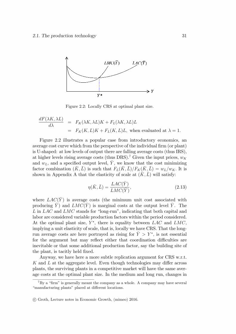
Figure 2.2 illustrates a popular case from introductory economics, anaverage cost curve which from the perspective of the individual firm (or plant)is U-shaped: at low levels of output there are falling average costs (thus IRS),at higher levels rising average costs (thus DRS).7 Given the input prices, wKand wL, and a specified output level, Y , we know that the cost minimizingfactor combination (K, L) is such that FL(K, L)/FK(K, L) = wL/wK . It isshown in Appendix A that the elasticity of scale at (K, L) will satisfy:
η(K, L) =LAC(Y )
LMC(Y ), (2.13)
where LAC(Y ) is average costs (the minimum unit cost associated withproducing Y ) and LMC(Y ) is marginal costs at the output level Y . TheL in LAC and LMC stands for “long-run”, indicating that both capital andlabor are considered variable production factors within the period considered.At the optimal plant size, Y ∗, there is equality between LAC and LMC,implying a unit elasticity of scale, that is, locally we have CRS. That the long-run average costs are here portrayed as rising for Y > Y ∗, is not essentialfor the argument but may reflect either that coordination diffi culties areinevitable or that some additional production factor, say the building site ofthe plant, is tacitly held fixed.Anyway, we have here a more subtle replication argument for CRS w.r.t.
K and L at the aggregate level. Even though technologies may differ acrossplants, the surviving plants in a competitive market will have the same aver-age costs at the optimal plant size. In the medium and long run, changes in
7By a “firm”is generally meant the company as a whole. A company may have several“manufacturing plants”placed at different locations.
c© Groth, Lecture notes in Economic Growth, (mimeo) 2016.
32CHAPTER 2. REVIEW OF TECHNOLOGY AND
FACTOR SHARES OF INCOME
aggregate output will take place primarily by entry and exit of optimal-sizeplants. Then, with a large number of relatively small plants, each produc-ing at approximately constant unit costs for small output variations, we canwithout substantial error assume constant returns to scale at the aggregatelevel. So the argument goes. Notice, however, that even in this form thereplication argument is not entirely convincing since the question of indivis-ibility remains. The optimal plant size may be large relative to the market− and is in fact so in many industries. Besides, in this case also the perfectcompetition premise breaks down.
2.1.3 Properties of the production function under CRS
The empirical evidence concerning returns to scale is mixed. Notwithstand-ing the theoretical and empirical ambiguities, the assumption of CRS w.r.t.capital and labor has a prominent role in macroeconomics. In many con-texts it is regarded as an acceptable approximation and a convenient simplebackground for studying the question at hand.Expedient inferences of the CRS assumption include:
(i) marginal costs are constant and equal to average costs (so the right-hand side of (2.13) equals unity);
(ii) if production factors are paid according to their marginal productivi-ties, factor payments exactly exhaust total output so that pure profitsare neither positive nor negative (so the right-hand side of (2.12) equalsunity);
(iii) a production function known to exhibit CRS and satisfy property (a)from the definition of a neoclassical production function above, will au-tomatically satisfy also property (b) and consequently be neoclassical;
(iv) a neoclassical two-factor production function with CRS has alwaysFKL > 0, i.e., it exhibits “direct complementarity” between K andL;
(v) a two-factor production function known to have CRS and to be twicecontinuously differentiable with positive marginal productivity of eachfactor everywhere in such a way that all isoquants are strictly convex tothe origin, must have diminishing marginal productivities everywhere.8
8Proofs of these claims can be found in intermediate microeconomics textbooks and inthe Appendix to Chapter 2 of my Lecture Notes in Macroeconomics.
c© Groth, Lecture notes in Economic Growth, (mimeo) 2016.
2.1. The production technology 33
A principal implication of the CRS assumption is that it allows a re-duction of dimensionality. Considering a neoclassical production function,Y = F (K,L) with L > 0, we can under CRS write F (K,L) = LF (K/L, 1)≡ Lf(k), where k ≡ K/L is called the capital-labor ratio (sometimes the cap-ital intensity) and f(k) is the production function in intensive form (some-times named the per capita production function). Thus output per unit oflabor depends only on the capital intensity:
y ≡ Y
L= f(k).
When the original production function F is neoclassical, under CRS theexpression for the marginal productivity of capital simplifies:
FK(K,L) =∂Y
∂K=∂ [Lf(k)]
∂K= Lf ′(k)
∂k
∂K= f ′(k). (2.14)
And the marginal productivity of labor can be written
FL(K,L) =∂Y
∂L=∂ [Lf(k)]
∂L= f(k) + Lf ′(k)
∂k
∂L= f(k) + Lf ′(k)K(−L−2) = f(k)− f ′(k)k. (2.15)
A neoclassical CRS production function in intensive form always has a posi-tive first derivative and a negative second derivative, i.e., f ′ > 0 and f ′′ < 0.The property f ′ > 0 follows from (2.14) and (2.2). And the property f ′′ < 0follows from (2.3) combined with
FKK(K,L) =∂f ′(k)
∂K= f ′′(k)
∂k
∂K= f ′′(k)
1
L.
For a neoclassical production function with CRS, we also have
f(k)− f ′(k)k > 0 for all k > 0, (2.16)
in view of f(0) ≥ 0 and f ′′ < 0. Moreover,
limk→0
[f(k)− f ′(k)k] = f(0). (2.17)
Indeed, from the mean value theorem9 we know that for any k > 0 thereexists a number a ∈ (0, 1) such that f ′(ak) = (f(k) − f(0))/k. For this awe thus have f(k) − f ′(ak)k = f(0) < f(k) − f ′(k)k, where the inequality
9This theorem says that if f is continuous in [α, β] and differentiable in (α, β), thenthere exists at least one point γ in (α, β) such that f ′(γ) = (f(β)− f(α))/(β − α).
c© Groth, Lecture notes in Economic Growth, (mimeo) 2016.
34CHAPTER 2. REVIEW OF TECHNOLOGY AND
FACTOR SHARES OF INCOME
follows from f ′(ak) > f ′(k), by f ′′ < 0. In view of f(0) ≥ 0, this establishes(2.16). And from f(k) > f(k) − f ′(k)k > f(0) and continuity of f (so thatlimk→0+ f(k) = f(0)) follows (2.17).Under CRS the Inada conditions for MPK can be written
limk→0
f ′(k) =∞, limk→∞
f ′(k) = 0. (2.18)
In this case standard parlance is just to say that “f satisfies the Inada con-ditions”.An input which must be positive for positive output to arise is called an
essential input ; an input which is not essential is called an inessential input.The second part of (2.18), representing the upper Inada condition for MPKunder CRS, has the implication that labor is an essential input; but capitalneed not be, as the production function f(k) = a+ bk/(1 + k), a > 0, b > 0,illustrates. Similarly, under CRS the upper Inada condition forMPL impliesthat capital is an essential input. These claims are proved in Appendix C.Combining these results, when both the upper Inada conditions hold andCRS obtain, then both capital and labor are essential inputs.10
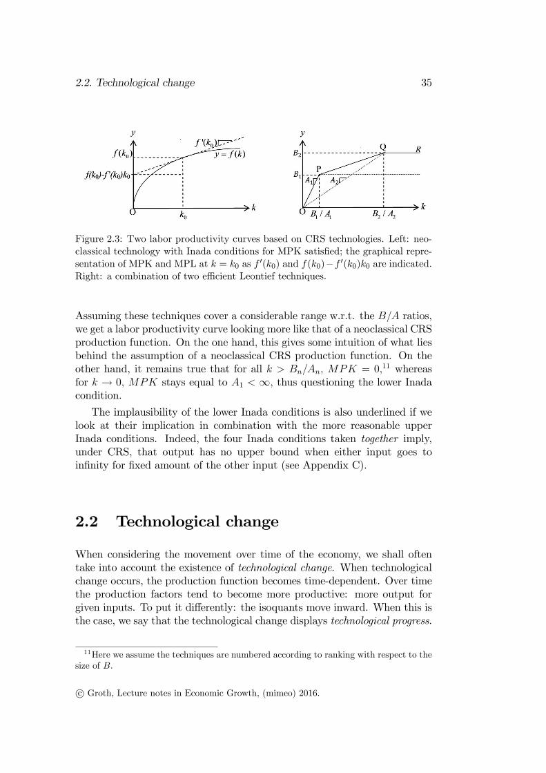
Figure 2.3 is drawn to provide an intuitive understanding of a neoclassicalCRS production function and at the same time illustrate that the lower Inadaconditions are more questionable than the upper Inada conditions. The leftpanel of Figure 2.3 shows output per unit of labor for a CRS neoclassical pro-duction function satisfying the Inada conditions for MPK. The f(k) in thediagram could for instance represent the Cobb-Douglas function in Example1 with β = 1−α, i.e., f(k) = Akα. The right panel of Figure 2.3 shows a non-neoclassical case where only two alternative Leontief techniques are available,technique 1: y = min(A1k,B1), and technique 2: y = min(A2k,B2). In theexposed case it is assumed that B2 > B1 and A2 < A1 (if A2 ≥ A1 at thesame time as B2 > B1, technique 1 would not be effi cient, because the sameoutput could be obtained with less input of at least one of the factors byshifting to technique 2). If the available K and L are such that k < B1/A1
or k > B2/A2, some of either L or K, respectively, is idle. If, however, theavailableK and L are such that B1/A1 < k < B2/A2, it is effi cient to combinethe two techniques and use the fraction µ of K and L in technique 1 and theremainder in technique 2, where µ = (B2/A2 − k)/(B2/A2 −B1/A1). In thisway we get the “labor productivity curve”OPQR (the envelope of the twotechniques) in Figure 2.3. Note that for k → 0, MPK stays equal to A1 <∞,whereas for all k > B2/A2, MPK = 0. A similar feature remains true, whenwe consider many, say n, alternative effi cient Leontief techniques available.
10Given a Cobb-Douglas production function, both production factors are essentialwhether we have DRS, CRS, or IRS.
c© Groth, Lecture notes in Economic Growth, (mimeo) 2016.
2.2. Technological change 35
Figure 2.3: Two labor productivity curves based on CRS technologies. Left: neo-classical technology with Inada conditions for MPK satisfied; the graphical repre-sentation of MPK and MPL at k = k0 as f ′(k0) and f(k0)−f ′(k0)k0 are indicated.Right: a combination of two effi cient Leontief techniques.
Assuming these techniques cover a considerable range w.r.t. the B/A ratios,we get a labor productivity curve looking more like that of a neoclassical CRSproduction function. On the one hand, this gives some intuition of what liesbehind the assumption of a neoclassical CRS production function. On theother hand, it remains true that for all k > Bn/An, MPK = 0,11 whereasfor k → 0, MPK stays equal to A1 < ∞, thus questioning the lower Inadacondition.
The implausibility of the lower Inada conditions is also underlined if welook at their implication in combination with the more reasonable upperInada conditions. Indeed, the four Inada conditions taken together imply,under CRS, that output has no upper bound when either input goes toinfinity for fixed amount of the other input (see Appendix C).
2.2 Technological change
When considering the movement over time of the economy, we shall oftentake into account the existence of technological change. When technologicalchange occurs, the production function becomes time-dependent. Over timethe production factors tend to become more productive: more output forgiven inputs. To put it differently: the isoquants move inward. When this isthe case, we say that the technological change displays technological progress.
11Here we assume the techniques are numbered according to ranking with respect to thesize of B.
c© Groth, Lecture notes in Economic Growth, (mimeo) 2016.
36CHAPTER 2. REVIEW OF TECHNOLOGY AND
FACTOR SHARES OF INCOME
Concepts of neutral technological change
A first step in taking technological change into account is to replace (2.1) by(2.4). Empirical studies often specialize (2.4) by assuming that technologicalchange take a form known as factor-augmenting technological change:
Yt = F (AtKt, BtLt), (2.19)
where F is a (time-independent) neoclassical production function, Yt, Kt,and Lt are output, capital, and labor input, respectively, at time t, while Atand Bt are time-dependent “effi ciencies” of capital and labor, respectively,reflecting technological change.In macroeconomics an even more specific form is often assumed, namely
the form of Harrod-neutral technological change.12 This amounts to assumingthat At in (2.19) is a constant (which we can then normalize to one). So onlyBt, which is then conveniently denoted Tt, is changing over time, and we have
Yt = F (Kt, TtLt). (2.20)
The effi ciency of labor, Tt, is then said to indicate the technology level. Al-though one can imagine natural disasters implying a fall in Tt, generallyTt tends to rise over time and then we say that (2.20) represents Harrod-neutral technological progress. An alternative name often used for this islabor-augmenting technological progress. The names “factor-augmenting”and, as here, “labor-augmenting” have become standard and we shall usethem when convenient, although they may easily be misunderstood. To saythat a change in Tt is labor-augmenting might be understood as meaningthat more labor is required to reach a given output level for given capital.In fact, the opposite is the case, namely that Tt has risen so that less laborinput is required. The idea is that the technological change affects the outputlevel as if the labor input had been increased exactly by the factor by whichT was increased, and nothing else had happened. (We might be tempted tosay that (2.20) reflects “labor saving” technological change. But also thiscan be misunderstood. Indeed, keeping L unchanged in response to a risein T implies that the same output level requires less capital and thus thetechnological change is “capital saving”.)If the function F in (2.20) is homogeneous of degree one (so that the
technology exhibits CRS w.r.t. capital and labor), we may write
yt ≡YtTtLt
= F (Kt
TtLt, 1) = F (kt, 1) ≡ f(kt), f ′ > 0, f ′′ < 0.
12After the English economist Roy F. Harrod, 1900-1978.
c© Groth, Lecture notes in Economic Growth, (mimeo) 2016.
2.2. Technological change 37
where kt ≡ Kt/(TtLt) ≡ kt/Tt (habitually called the “effective” capital in-tensity or, if there is no risk of confusion, just the capital intensity). Inrough accordance with a general trend in aggregate productivity data forindustrialized countries we often assume that T grows at a constant rate, g,so that in discrete time Tt = T0(1 + g)t and in continuous time Tt = T0e
gt,where g > 0. The popularity in macroeconomics of the hypothesis of labor-augmenting technological progress derives from its consistency with Kaldor’s“stylized facts”, cf. Chapter 4.There exists two alternative concepts of neutral technological progress.
Hicks-neutral technological progress is said to occur if technological develop-ment is such that the production function can be written in the form
Yt = TtF (Kt, Lt), (2.21)
where, again, F is a (time-independent) neoclassical production function,while Tt is the growing technology level.13 The assumption of Hicks-neutralityhas been used more in microeconomics and partial equilibrium analysis thanin macroeconomics. If F has CRS, we can write (2.21) as Yt = F (TtKt, TtLt).Comparing with (2.19), we see that in this case Hicks-neutrality is equivalentto At = Bt in (2.19), whereby technological change is said to be equallyfactor-augmenting.Finally, in a symmetric analogy with (2.20), what is known as capital-
augmenting technological progress is present when
Yt = F (TtKt, Lt). (2.22)
Here technological change acts as if the capital input were augmented. Forsome reason this form is sometimes called Solow-neutral technological progress.14
This association of (2.22) to Solow’s name is misleading, however. In his fa-mous growth model,15 Solow assumed Harrod-neutral technological progress.And in another famous contribution, Solow generalized the concept of Harrod-neutrality to the case of embodied technological change and capital of differentvintages, see below.It is easily shown (Exercise I.9) that the Cobb-Douglas production func-
tion (2.8) (with time-independent output elasticities w.r.t. K and L) satisfiesall three neutrality criteria at the same time, if it satisfies one of them (whichit does if technological change does not affect α and β). It can also be shownthat within the class of neoclassical CRS production functions the Cobb-Douglas function is the only one with this property (see Exercise ??).
13After the English economist and Nobel Prize laureate John R. Hicks, 1904-1989.14After the American economist and Nobel Prize laureate Robert Solow (1924-).15Solow (1956).
c© Groth, Lecture notes in Economic Growth, (mimeo) 2016.
38CHAPTER 2. REVIEW OF TECHNOLOGY AND
FACTOR SHARES OF INCOME
Note that the neutrality concepts do not say anything about the sourceof technological progress, only about the quantitative form in which it ma-terializes. For instance, the occurrence of Harrod-neutrality should not beinterpreted as indicating that the technological change emanates specificallyfrom the labor input in some sense. Harrod-neutrality only means that tech-nological innovations predominantly are such that not only do labor andcapital in combination become more productive, but this happens to man-ifest itself in the form (2.20), that is, as if an improvement in the qualityof the labor input had occurred. (Even when improvement in the qualityof the labor input is on the agenda, the result may be a reorganization ofthe production process ending up in a higher Bt along with, or instead of, ahigher At in the expression (2.19).)
Rival versus nonrival goods
When a production function (or more generally a production possibility set)is specified, a given level of technical knowledge is presumed. As this levelchanges over time, the production function changes. In (2.4) this dependencyon the level of knowledge was represented indirectly by the time dependencyof the production function. Sometimes it is useful to let the knowledge de-pendency be explicit by perceiving knowledge as an additional productionfactor and write, for instance,
Yt = F (Xt, Tt), (2.23)
where Tt is now an index of the amount of knowledge, while Xt is a vectorof ordinary inputs like raw materials, machines, labor etc. In this contextthe distinction between rival and nonrival inputs or more generally the dis-tinction between rival and nonrival goods is important. A good is rival ifits character is such that one agent’s use of it inhibits other agents’use ofit at the same time. A pencil is thus rival. Many production inputs likeraw materials, machines, labor etc. have this property. They are elements ofthe vector Xt. By contrast, however, technical knowledge is a nonrival good.An arbitrary number of factories can simultaneously use the same piece oftechnical knowledge in the sense of a list of instructions about how differentinputs can be combined to produce a certain output. An engineering principleor a farmaceutical formula are examples. (Note that the distinction rival-nonrival is different from the distinction excludable-nonexcludable. A goodis excludable if other agents, firms or households, can be excluded from usingit. Other firms can thus be excluded from commercial use of a certain piece oftechnical knowledge if it is patented. The existence of a patent concerns the
c© Groth, Lecture notes in Economic Growth, (mimeo) 2016.

2.2. Technological change 39
legal status of a piece of knowledge and does not interfere with its economiccharacter as a nonrival input.).What the replication argument really says is that by, conceptually, dou-
bling all the rival inputs, we should always be able to double the output,since we just “replicate”what we are already doing. This is then an argu-ment for (at least) CRS w.r.t. the elements of Xt in (2.23). The point is thatbecause of its nonrivalry, we do not need to increase the stock of knowledge.Now let us imagine that the stock of knowledge is doubled at the same timeas the rival inputs are doubled. Then more than a doubling of output shouldoccur. In this sense we may speak of IRS w.r.t. the rival inputs and T takentogether.Before proceeding, we briefly comment on how the capital stock, Kt,
is typically measured. While data on gross investment, It, is available innational income and product accounts, data on Kt usually is not. One ap-proach to the measurement of Kt is the perpetual inventory method whichbuilds upon the accounting relationship
Kt = It−1 + (1− δ)Kt−1. (2.24)
Assuming a constant capital depreciation rate δ, backward substitution gives
Kt = It−1+(1−δ) [It−2 + (1− δ)Kt−2] = . . . =N∑i=1
(1−δ)i−1It−i+(1−δ)NKt−N .
(2.25)Based on a long time series for I and an estimate of δ, one can insert theseobserved values in the formula and calculate Kt, starting from a rough con-jecture about the initial value Kt−N . The result will not be very sensitive tothis conjecture since for large N the last term in (2.25) becomes very small.
Embodied vs. disembodied technological progress
There exists an additional taxonomy of technological change. We say thattechnological change is embodied, if taking advantage of new technical knowl-edge requires construction of new investment goods. The new technology isincorporated in the design of newly produced equipment, but this equipmentwill not participate in subsequent technological progress. An example: onlythe most recent vintage of a computer series incorporates the most recentadvance in information technology. Then investment goods produced later(investment goods of a later “vintage”) have higher productivity than in-vestment goods produced earlier at the same resource cost. Thus investmentbecomes an important driving force in productivity increases.
c© Groth, Lecture notes in Economic Growth, (mimeo) 2016.
40CHAPTER 2. REVIEW OF TECHNOLOGY AND
FACTOR SHARES OF INCOME
We way formalize embodied technological progress by writing capital ac-cumulation in the following way:
Kt+1 −Kt = qtIt − δKt, (2.26)
where It is gross investment in period t, i.e., It = Yt − Ct, and qt measuresthe “quality”(productivity) of newly produced investment goods. The risinglevel of technology implies rising q so that a given level of investment givesrise to a greater and greater addition to the capital stock, K, measuredin effi ciency units. In aggregate models C and I are produced with thesame technology, the aggregate production function. From this together with(2.26) follows that q capital goods can be produced at the same minimumcost as one consumption good. Hence, the equilibrium price, p, of capitalgoods in terms of the consumption good must equal the inverse of q, i.e.,p = 1/q. The output-capital ratio in value terms is Y/(pK) = qY/K.Note that even if technological change does not directly appear in the
production function, that is, even if for instance (2.20) is replaced by Yt= F (Kt, Lt), the economy may experience a rising standard of living when qis growing over time.In contrast, disembodied technological change occurs when new technical
and organizational knowledge increases the combined productivity of the pro-duction factors independently of when they were constructed or educated. IftheKt appearing in (2.20), (2.21), and (2.22) above refers to the total, histor-ically accumulated capital stock as calculated by (2.25), then the evolutionof T in these expressions can be seen as representing disembodied technolog-ical change. All vintages of the capital equipment benefit from a rise in thetechnology level Tt. No new investment is needed to benefit.Based on data for the U.S. 1950-1990, and taking quality improvements
into account, Greenwood et al. (1997) estimate that embodied technologicalprogress explains about 60% of the growth in output per man hour. So,empirically, embodied technological progress seems to play a dominant role.As this tends not to be fully incorporated in national income accounting atfixed prices, there is a need to adjust the investment levels in (2.25) to bettertake estimated quality improvements into account. Otherwise the resultingK will not indicate the capital stock measured in effi ciency units.
2.3 The concepts of representative firm andaggregate production function*
Many macroeconomic models make use of the simplifying notion of a rep-resentative firm. By this is meant a fictional firm whose production “rep-
c© Groth, Lecture notes in Economic Growth, (mimeo) 2016.
2.3. The concepts of representative firm and aggregate production function*41
resents” aggregate production (value added) in a sector or in society as awhole.Suppose there are n firms in the sector considered or in society as a
whole. Let F i be the production function for firm i so that Yi = F i(Ki, Li),where Yi, Ki, and Li are output, capital input, and labor input, respectively,i = 1, 2, . . . , n. Further, let Y = Σn
i=1Yi, K = Σni=1Ki, and L = Σn
i=1Li.Ignoring technological change, suppose the aggregate variables are relatedthrough some function, F ∗, such that we can write
Y = F ∗(K,L),
and such that the choices of a single firm facing this production functioncoincide with the aggregate outcomes, Σn
i=1Yi, Σni=1Ki, and Σn
i=1Li, in theoriginal economy. Then F ∗(K,L) is called the aggregate production functionor the production function of the representative firm. It is as if aggregateproduction is the result of the behavior of such a single firm.A simple example where the aggregate production function is well-defined
is the following. Suppose that all firms have the same production functionso that Yi = F (Ki, Li), i = 1, 2, . . . , n. If in addition F has CRS, we have
Yi = F (Ki, Li) = LiF (ki, 1) ≡ Lif(ki),
where ki ≡ Ki/Li. Hence, facing given factor prices, cost-minimizing firmswill choose the same capital intensity ki = k for all i. From Ki = kLi thenfollows
∑iKi = k
∑i Li so that k = K/L. Thence,
Y ≡∑
Yi =∑
Lif(ki) = f(k)∑
Li = f(k)L = F (k, 1)L = F (K,L).
In this (trivial) case the aggregate production function is well-defined andturns out to be exactly the same as the identical CRS production functionsof the individual firms. Moreover, given CRS and ki = k for all i, we have∂Yi/∂Ki = f ′(ki) = f ′(k) = FK(K,L) for all i. So each firm’s marginalproductivity of capital is the same as the marginal productivity of capital onthe basis of the aggregate production function.Allowing for the existence of different production functions at firm level,
we may define the aggregate production function as
F (K,L) = max(K1,L1,...,Kn,Ln)≥0
F 1(K1, L1) + · · ·+ F n(Kn, Ln)
s.t.∑i
Ki ≤ K,∑i
Li ≤ L.
Allowing also for existence of different output goods, different capitalgoods, and different types of labor makes the issue more intricate, of course.
c© Groth, Lecture notes in Economic Growth, (mimeo) 2016.
42CHAPTER 2. REVIEW OF TECHNOLOGY AND
FACTOR SHARES OF INCOME
Yet, if firms are price taking profit maximizers and there are nonincreasingreturns to scale, we at least know that the aggregate outcome is as if, forgiven prices, the firms jointly maximize aggregate profit on the basis of theircombined production technology (Mas-Colell et al., 1955). The problem is,however, that the conditions needed for this to imply existence of an ag-gregate production function which is well-behaved (in the sense of inheritingsimple qualitative properties from its constituent parts) are restrictive.Nevertheless macroeconomics often treats aggregate output as a single ho-
mogeneous good and capital and labor as being two single and homogeneousinputs. There was in the 1960s a heated debate about the problems involvedin this, with particular emphasis on the aggregation of different kinds ofequipment into one variable, the capital stock “K”. The debate is knownas the “Cambridge controversy”because the dispute was between a group ofeconomists from Cambridge University, UK, and a group from MassachusettsInstitute of Technology (MIT), which is located in Cambridge, USA. The for-mer group questioned the theoretical robustness of several of the neoclassicaltenets, including the proposition that rising aggregate capital intensity tendsto be associated with a falling rate of interest. Starting at the disaggregatelevel, an association of this sort is not a logical necessity because, with differ-ent production functions across the industries, the relative prices of producedinputs tend to change, when the interest rate changes. While acknowledgingthe possibility of “paradoxical” relationships, the latter group maintainedthat in a macroeconomic context they are likely to cause devastating prob-lems only under exceptional circumstances. In the end this is a matter ofempirical assessment.16
To avoid complexity and because, for many important issues in growththeory, there is today no well-tried alternative, we shall in this course mostof the time use aggregate constructs like “Y ”, “K”, and “L” as simplify-ing devices, hopefully acceptable in a first approximation. There are cases,however, where some disaggregation is pertinent. When for example the roleof imperfect competition is in focus, we shall be ready to disaggregate theproduction side of the economy into several product lines, each producing itsown differentiated product. We shall also touch upon a type of growth modelswhere a key ingredient is the phenomenon of “creative destruction”meaningthat an incumbent technological leader is competed out by an entrant witha qualitatively new technology.Like the representative firm, the representative household and the aggre-
16In his review of the Cambridge controversy Mas-Colell (1989) concluded that: “Whatthe ‘paradoxical’ comparative statics [of disaggregate capital theory] has taught us issimply that modelling the world as having a single capital good is not a priori justified.So be it.”
c© Groth, Lecture notes in Economic Growth, (mimeo) 2016.
2.4. Long-run vs. short-run production functions* 43
gate consumption function are simplifying notions that should be appliedonly when they do not get in the way of the issue to be studied. The im-portance of budget constraints may make it even more diffi cult to aggregateover households than over firms. Yet, if (and that is a big if) all householdshave the same, constant marginal propensity to consume out of income, ag-gregation is straightforward and the representative household is a meaningfulconcept. On the other hand, if we aim at understanding, say, the interactionbetween lending and borrowing households, perhaps via financial intermedi-aries, the representative household is not a useful starting point. Similarly,if the theme is conflicts of interests between firm owners and employees, theexistence of different types of households should be taken into account.
2.4 Long-run vs. short-run production func-tions*
Is the substitutability between capital and labor the same “ex ante”and “expost”? By ex ante is meant “when plant and machinery are to be decidedupon”and by ex post is meant “after the equipment is designed and con-structed”. In the standard neoclassical competitive setup, of for instancethe Solow or the Ramsey model, there is a presumption that also after theconstruction and installation of the equipment in the firm, the ratio of thefactor inputs can be fully adjusted to a change in the relative factor price. Inpractice, however, when some machinery has been constructed and installed,its functioning will often require a more or less fixed number of machine op-erators. What can be varied is just the degree of utilization of the machinery.That is, after construction and installation of the machinery, the choice op-portunities are no longer described by the neoclassical production functionbut by a Leontief production function,
Y = min(AuK,BL), A > 0, B > 0, (2.27)
where K is the size of the installed machinery (a fixed factor in the shortrun) measured in effi ciency units, u is its utilization rate (0 ≤ u ≤ 1), and Aand B are given technical coeffi cients measuring effi ciency.So in the short run the choice variables are u and L. In fact, essentially
only u is a choice variable since effi cient production trivially requires L =AuK/B. Under “full capacity utilization”we have u = 1 (each machine isused 24 hours per day seven days per week). “Capacity”is given as AK perweek. Producing effi ciently at capacity requiresL = AK/B and the marginalproduct by increasing labor input is here nil. But if demand, Y d, is less than
c© Groth, Lecture notes in Economic Growth, (mimeo) 2016.
44CHAPTER 2. REVIEW OF TECHNOLOGY AND
FACTOR SHARES OF INCOME
capacity, satisfying this demand effi ciently requires u = Y d/(AK) < 1 and L= Y d/B. As long as u < 1, the marginal productivity of labor is a constant,B.The various effi cient input proportions that are possible ex ante may be
approximately described by a neoclassical CRS production function. Let thisfunction on intensive form be denoted y = f(k).When investment is decidedupon and undertaken, there is thus a choice between alternative effi cient pairsof the technical coeffi cients A and B in (2.27). These pairs satisfy
f(k) = Ak = B. (2.28)
So, for an increasing sequence of k’s, k1, k2,. . . , ki,. . . , the correspondingpairs are (Ai, Bi) = (f(ki)/ki, f(ki)), i = 1, 2,. . . .17 We say that ex ante,depending on the relative factor prices as they are “now”and are expectedto evolve in the future, a suitable technique, (Ai, Bi), is chosen from anopportunity set described by the given neoclassical production function. Butex post, i.e., when the equipment corresponding to this technique is installed,the production opportunities are described by a Leontief production functionwith (A,B) = (Ai, Bi).In the picturesque language of Phelps (1963), technology is in this case
putty-clay. Ex ante the technology involves capital which is “putty” in thesense of being in a malleable state which can be transformed into a range ofvarious machinery requiring capital-labor ratios of different magnitude. Butonce the machinery is constructed, it enters a “hardened”state and becomes”clay”. Then factor substitution is no longer possible; the capital-labor ra-tio at full capacity utilization is fixed at the level k = Bi/Ai, as in (2.27).Following the terminology of Johansen (1972), we say that a putty-clay tech-nology involves a “long-run production function”which is neoclassical and a“short-run production function”which is Leontief.In contrast, the standard neoclassical setup assumes the same range of
substitutability between capital and labor ex ante and ex post. Then thetechnology is called putty-putty. This term may also be used if ex post thereis at least some substitutability although less than ex ante. At the oppositepole of putty-putty we may consider a technology which is clay-clay. Hereneither ex ante nor ex post is factor substitution possible. Table 2.1 gives anoverview of the alternative cases.
Table 2.1. Technologies classified according to
17The points P and Q in the right-hand panel of Fig. 2.3 can be interpreted as con-structed this way from the neoclassical production function in the left-hand panel of thefigure.
c© Groth, Lecture notes in Economic Growth, (mimeo) 2016.
2.5. The neoclassical theory of factor income shares 45
factor substitutability ex ante and ex postEx post substitution
Ex ante substitution possible impossiblepossible putty-putty putty-clayimpossible clay-clay
The putty-clay case is generally considered the realistic case. As timeproceeds, technological progress occurs. To take this into account, we mayreplace (2.28) and (2.27) by f(kt, t) = Atkt = Bt and Yt = min(AtutKt, BtLt),respectively. If a new pair of Leontief coeffi cients, (At2 , Bt2), effi ciency-dominates its predecessor (by satisfying At2 ≥ At1 and Bt2 ≥ Bt1 with atleast one strict equality), it may pay the firm to invest in the new technol-ogy at the same time as some old machinery is scrapped. Real wages tendto rise along with technological progress and the scrapping occurs becausethe revenue from using the old machinery in production no longer covers theassociated labor costs.The clay property ex-post of many technologies is important for short-run
analysis. It implies that there may be non-decreasing marginal productivityof labor up to a certain point. It also implies that in its investment decisionthe firm will have to take expected future technologies and future factor pricesinto account. For many issues in long-run analysis the clay property ex-postmay be less important, since over time adjustment takes place through newinvestment.
2.5 The neoclassical theory of factor incomeshares
To begin with, we ignore technological progress and write aggregate outputas Y = F (K,L), where F is neoclassical with CRS. From Euler’s theoremfollows that F (K,L) = F1K + F2L = f ′(k)K + (f(k) − kf ′(k))L, wherek ≡ K/L. In equilibrium under perfect competition we have
Y = rK + wL,
where r = r + δ = f ′(k) ≡ r(k) is the cost per unit of capital input and w= f(k)−kf ′(k) ≡ w(k) is the real wage, i.e., the cost per unit of labor input.We have r′(k) = f ′′(k) < 0 and w′(k) = −kf ′′(k) > 0.The labor income share is
wL
Y=f(k)− kf ′(k)
f(k)≡ w(k)
f(k)≡ SL(k) =
wL
rK + wL=
w/rk
1 + w/rk
, (2.29)
c© Groth, Lecture notes in Economic Growth, (mimeo) 2016.
46CHAPTER 2. REVIEW OF TECHNOLOGY AND
FACTOR SHARES OF INCOME
where the function SL(·) is the income share of labor function, w/r is thefactor price ratio, and (w/r)/k = w/(rk) is the factor income ratio. As r′(k)= f ′′(k) < 0 and w′(k) = −kf ′′(k) > 0, the factor price ratio, w/r, is anincreasing function of k.Suppose that capital tends to grow faster than labor so that k rises over
time. Unless the production function is Cobb-Douglas, this will under perfectcompetition affect the labor income share. But apriori it is not obvious inwhat direction. By (2.29) we see that the labor income share moves inthe same direction as the factor income ratio, (w/r)/k. The latter goes up(down) depending on whether the percentage rise in the factor price ratiow/r is greater (smaller) than the percentage rise in k. So, if we let E`xg(x)denote the elasticity of a function g(x) w.r.t. x, we can only say that
SL′(k) R 0 for E`kw
rR 1, (2.30)
respectively. In words: if the production function is such that the ratio ofthe marginal productivities of the two production factors is strongly (weakly)sensitive to the capital-labor ratio, then the labor income share rises (falls)along with a rise in K/L.Usually, however, the inverse elasticity is considered, namely E`w/rk (=
1/E`k wr ). This elasticity indicates how sensitive the cost minimizing capital-labor ratio, k, is to a given factor price ratio w/r. Under perfect competitionE`w/rk coincides with what is known as the elasticity of factor substitution(for a general definition, see below). The latter is often denoted σ. In theCRS case, σ will be a function of only k so that we can write E`w/rk = σ(k).By (2.30), we therefore have
SL′(k) R 0 for σ(k) Q 1,
respectively.The size of the elasticity of factor substitution is a property of the pro-
duction function, hence of the technology. In special cases the elasticity offactor substitution is a constant, i.e., independent of k. For instance, if F isCobb-Douglas, i.e., Y = KαL1−α, 0 < α < 1, we have σ(k) ≡ 1, as shownin Section 2.7. In this case variation in k does not change the labor incomeshare under perfect competition. Empirically there is not agreement aboutthe “normal” size of the elasticity of factor substitution for industrializedeconomies, but the bulk of studies seems to conclude with σ(k) < 1 (seebelow).
Adding Harrod-neutral technical progress We now add Harrod-neutraltechnical progress. We write aggregate output as Y = F (K,TL), where F
c© Groth, Lecture notes in Economic Growth, (mimeo) 2016.
2.5. The neoclassical theory of factor income shares 47
is neoclassical with CRS, and T = Tt = T0(1 + g)t. Then the labor incomeshare is
wL
Y=
w/T
Y/(TL)≡ w
y.
The above formulas still hold if we replace k by k ≡ K/(TL) and w by w≡ w/T. We get
SL′(k) R 0 for σ(k) Q 1,
respectively. We see that if σ(k) < 1 in the relevant range for k, then marketforces tend to increase the income share of the factor that is becoming rela-tively more scarce, which is effi ciency-adjusted labor, TL, if k is increasing.And if instead σ(k) > 1 in the relevant range for k, then market forces tendto decrease the income share of the factor that is becoming relatively morescarce.While k empirically is clearly growing, k ≡ k/T is not necessarily so
because also T is increasing. Indeed, according to Kaldor’s “stylized facts”,apart from short- and medium-term fluctuations, k − and therefore also rand the labor income share − tend to be more or less constant over time.This can happen whatever the sign of σ(k∗) − 1, where k∗ is the long-runvalue of the effective capital-labor ratio k. Given CRS and the productionfunction f, the elasticity of substitution between capital and labor does notdepend on whether g = 0 or g > 0, but only on the function f itself and thelevel of K/(TL).As alluded to earlier, there are empiricists who reject Kaldor’s “facts”
as a general tendency. For instance Piketty (2014) essentially claims thatin the very long run the effective capital-labor ratio k has an upward trend,temporarily braked by two world wars and the Great Depression in the 1930s.If so, the sign of σ(k)− 1 becomes decisive for in what direction wL/Y willmove. Piketty interprets the econometric literature as favoring σ(k) > 1,which means there should be downward pressure on wL/Y . This particularsource behind a falling wL/Y can be questioned, however. Indeed, σ(k) > 1contradicts the more general empirical view referred to above.18
Immigration
Here is another example that illustrates the importance of the size of σ(k).Consider an economy with perfect competition and a given aggregate capitalstock K and technology level T (entering the production function in thelabor-augmenting way as above). Suppose that for some reason, immigration,
18According to Summers (2014), Piketty’s interpretation relies on conflating gross andnet returns to capital.
c© Groth, Lecture notes in Economic Growth, (mimeo) 2016.
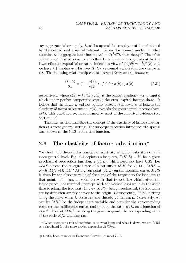
48CHAPTER 2. REVIEW OF TECHNOLOGY AND
FACTOR SHARES OF INCOME
say, aggregate labor supply, L, shifts up and full employment is maintainedby the needed real wage adjustment. Given the present model, in whatdirection will aggregate labor income wL = w(k)TL then change? The effectof the larger L is to some extent offset by a lower w brought about by thelower effective capital-labor ratio. Indeed, in view of dw/dk = −kf ′′(k) > 0,we have k ↓ implies w ↓ for fixed T. So we cannot apriori sign the change inwL. The following relationship can be shown (Exercise ??), however:
∂(wL)
∂L= (1− α(k)
σ(k))w R 0 for α(k) Q σ(k), (2.31)
respectively, where a(k) ≡ kf ′(k)/f(k) is the output elasticity w.r.t. capitalwhich under perfect competition equals the gross capital income share. Itfollows that the larger L will not be fully offset by the lower w as long as theelasticity of factor substitution, σ(k), exceeds the gross capital income share,α(k). This condition seems confirmed by most of the empirical evidence (seeSection 2.7).The next section describes the concept of the elasticity of factor substitu-
tion at a more general setting. The subsequent section introduces the specialcase known as the CES production function.
2.6 The elasticity of factor substitution*
We shall here discuss the concept of elasticity of factor substitution at amore general level. Fig. 2.4 depicts an isoquant, F (K,L) = Y , for a givenneoclassical production function, F (K,L), which need not have CRS. LetMRS denote the marginal rate of substitution of K for L, i.e., MRS =FL(K,L)/FK(K,L).19 At a given point (K,L) on the isoquant curve, MRSis given by the absolute value of the slope of the tangent to the isoquant atthat point. This tangent coincides with that isocost line which, given thefactor prices, has minimal intercept with the vertical axis while at the sametime touching the isoquant. In view of F (·) being neoclassical, the isoquantsare by definition strictly convex to the origin. Consequently, MRS is risingalong the curve when L decreases and thereby K increases. Conversely, wecan let MRS be the independent variable and consider the correspondingpoint on the indifference curve, and thereby the ratio K/L, as a function ofMRS. If we let MRS rise along the given isoquant, the corresponding valueof the ratio K/L will also rise.
19When there is no risk of confusion as to what is up and what is down, we use MRSas a shorthand for the more precise expression MRSKL.
c© Groth, Lecture notes in Economic Growth, (mimeo) 2016.
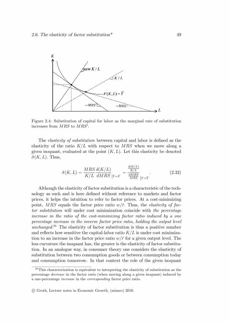
2.6. The elasticity of factor substitution* 49
Figure 2.4: Substitution of capital for labor as the marginal rate of substitutionincreases from MRS to MRS′.
The elasticity of substitution between capital and labor is defined as theelasticity of the ratio K/L with respect to MRS when we move along agiven isoquant, evaluated at the point (K,L). Let this elasticity be denotedσ(K,L). Thus,
σ(K,L) =MRS
K/L
d(K/L)
dMRS |Y=Y=
d(K/L)K/L
dMRSMRS |Y=Y
. (2.32)
Although the elasticity of factor substitution is a characteristic of the tech-nology as such and is here defined without reference to markets and factorprices, it helps the intuition to refer to factor prices. At a cost-minimizingpoint, MRS equals the factor price ratio w/r. Thus, the elasticity of fac-tor substitution will under cost minimization coincide with the percentageincrease in the ratio of the cost-minimizing factor ratio induced by a onepercentage increase in the inverse factor price ratio, holding the output levelunchanged.20 The elasticity of factor substitution is thus a positive numberand reflects how sensitive the capital-labor ratioK/L is under cost minimiza-tion to an increase in the factor price ratio w/r for a given output level. Theless curvature the isoquant has, the greater is the elasticity of factor substitu-tion. In an analogue way, in consumer theory one considers the elasticity ofsubstitution between two consumption goods or between consumption todayand consumption tomorrow. In that context the role of the given isoquant
20This characterization is equivalent to interpreting the elasticity of substitution as thepercentage decrease in the factor ratio (when moving along a given isoquant) induced bya one-percentage increase in the corresponding factor price ratio.
c© Groth, Lecture notes in Economic Growth, (mimeo) 2016.
50CHAPTER 2. REVIEW OF TECHNOLOGY AND
FACTOR SHARES OF INCOME
is taken over by an indifference curve. That is also the case when we con-sider the intertemporal elasticity of substitution in labor supply, cf. the nextchapter.Calculating the elasticity of substitution between K and L at the point
(K,L), we get
σ(K,L) = − FKFL(FKK + FLL)
KL [(FL)2FKK − 2FKFLFKL + (FK)2FLL], (2.33)
where all the derivatives are evaluated at the point (K,L). When F (K,L)has CRS, the formula (2.33) simplifies to
σ(K,L) =FK(K,L)FL(K,L)
FKL(K,L)F (K,L)= −f
′(k) (f(k)− f ′(k)k)
f ′′(k)kf(k)≡ σ(k), (2.34)
where k ≡ K/L.21 We see that under CRS, the elasticity of substitutiondepends only on the capital-labor ratio k, not on the output level. We willnow consider the case where the elasticity of substitution is independent alsoof the capital-labor ratio.
2.7 The CES production function
It can be shown22 that if a neoclassical production function with CRS has aconstant elasticity of factor substitution different from one, it must be of theform
Y = A[αKβ + (1− α)Lβ
] 1β , (2.35)
where A, α, and β are parameters satisfying A > 0, 0 < α < 1, and β < 1,β 6= 0. This function has been used intensively in empirical studies and iscalled a CES production function (CES for Constant Elasticity of Substitu-tion). For a given choice of measurement units, the parameter A reflectseffi ciency (or what is known as total factor productivity) and is thus calledthe effi ciency parameter. The parameters α and β are called the distribu-tion parameter and the substitution parameter, respectively. The restrictionβ < 1 ensures that the isoquants are strictly convex to the origin. Note thatif β < 0, the right-hand side of (16.32) is not defined when either K or L(or both) equal 0.We can circumvent this problem by extending the domainof the CES function and assign the function value 0 to these points whenβ < 0. Continuity is maintained in the extended domain (see Appendix E).
21The formulas (2.33) and (2.34) are derived in Appendix D of Chapter 4 of Groth,Lecture Notes in Macroeconomics..22See, e.g., Arrow et al. (1961).
c© Groth, Lecture notes in Economic Growth, (mimeo) 2016.
2.7. The CES production function 51
By taking partial derivatives in (16.32) and substituting back we get
∂Y
∂K= αAβ
(Y
K
)1−β
and∂Y
∂L= (1− α)Aβ
(Y
L
)1−β
, (2.36)
where Y/K = A[α + (1− α)k−β
] 1β and Y/L = A
[αkβ + 1− α
] 1β . The mar-
ginal rate of substitution of K for L therefore is
MRS =∂Y/∂L
∂Y/∂K=
1− αα
k1−β > 0.
Consequently,dMRS
dk=
1− αα
(1− β)k−β,
where the inverse of the right-hand side is the value of dk/dMRS. Substitut-ing these expressions into (16.34) gives
σ(K,L) =1
1− β ≡ σ, (2.37)
confirming the constancy of the elasticity of substitution. Since β < 1, σ > 0always. A higher substitution parameter, β, results in a higher elasticity offactor substitution, σ. And σ ≶ 1 for β ≶ 0, respectively.Since β = 0 is not allowed in (16.32), at first sight we cannot get σ = 1
from this formula. Yet, σ = 1 can be introduced as the limiting case of (16.32)when β → 0, which turns out to be the Cobb-Douglas function. Indeed, onecan show23 that, for fixed K and L,
A[αKβ + (1− α)Lβ
] 1β → AKαL1−α, for β → 0.
By a similar procedure as above we find that a Cobb-Douglas function alwayshas elasticity of substitution equal to 1; this is exactly the value taken byσ in (16.35) when β = 0. In addition, the Cobb-Douglas function is theonly production function that has unit elasticity of substitution whateverthe capital-labor ratio.Another interesting limiting case of the CES function appears when, for
fixed K and L, we let β → −∞ so that σ → 0. We get
A[αKβ + (1− α)Lβ
] 1β → Amin(K,L), for β → −∞. (2.38)
23For proofs of this and the further claims below, see Appendix E of Chapter 4 of Groth,Lecture Notes in Macroeconomics.
c© Groth, Lecture notes in Economic Growth, (mimeo) 2016.
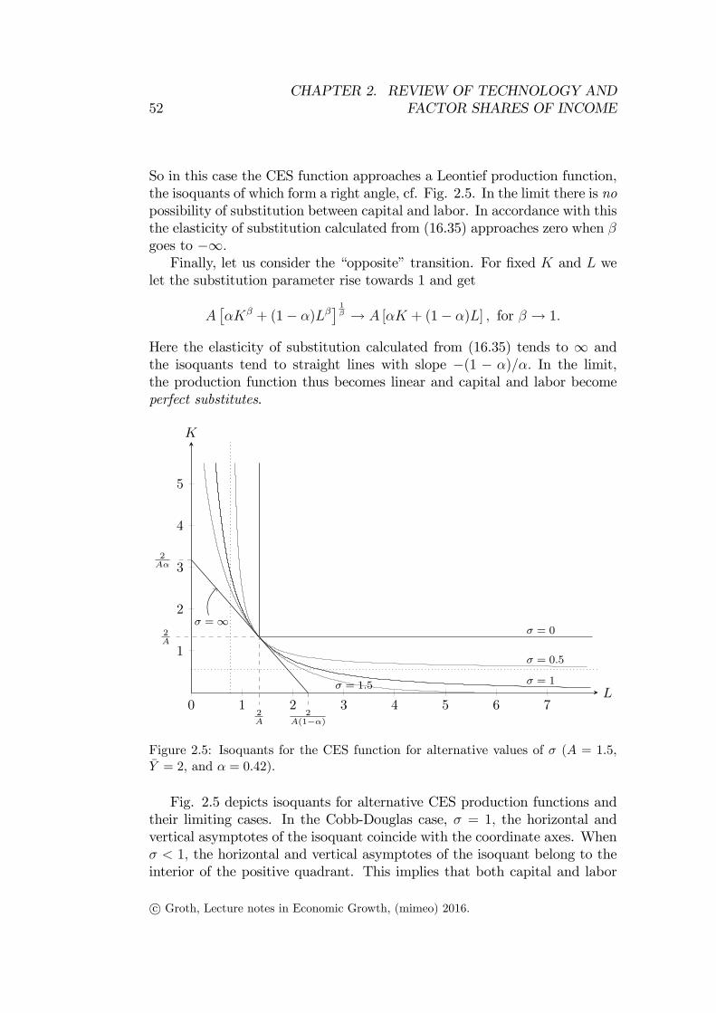
52CHAPTER 2. REVIEW OF TECHNOLOGY AND
FACTOR SHARES OF INCOME
So in this case the CES function approaches a Leontief production function,the isoquants of which form a right angle, cf. Fig. 2.5. In the limit there is nopossibility of substitution between capital and labor. In accordance with thisthe elasticity of substitution calculated from (16.35) approaches zero when βgoes to −∞.Finally, let us consider the “opposite”transition. For fixed K and L we
let the substitution parameter rise towards 1 and get
A[αKβ + (1− α)Lβ
] 1β → A [αK + (1− α)L] , for β → 1.
Here the elasticity of substitution calculated from (16.35) tends to ∞ andthe isoquants tend to straight lines with slope −(1 − α)/α. In the limit,the production function thus becomes linear and capital and labor becomeperfect substitutes.
0 1 2 3 4 5 6 7
1
2
3
4
5
σ = 0
σ = 0.5
σ = 1σ = 1.5
σ = ∞2A
2A
2Aα
2A(1−α)
L
K
Figure 2.5: Isoquants for the CES function for alternative values of σ (A = 1.5,Y = 2, and α = 0.42).
Fig. 2.5 depicts isoquants for alternative CES production functions andtheir limiting cases. In the Cobb-Douglas case, σ = 1, the horizontal andvertical asymptotes of the isoquant coincide with the coordinate axes. Whenσ < 1, the horizontal and vertical asymptotes of the isoquant belong to theinterior of the positive quadrant. This implies that both capital and labor
c© Groth, Lecture notes in Economic Growth, (mimeo) 2016.
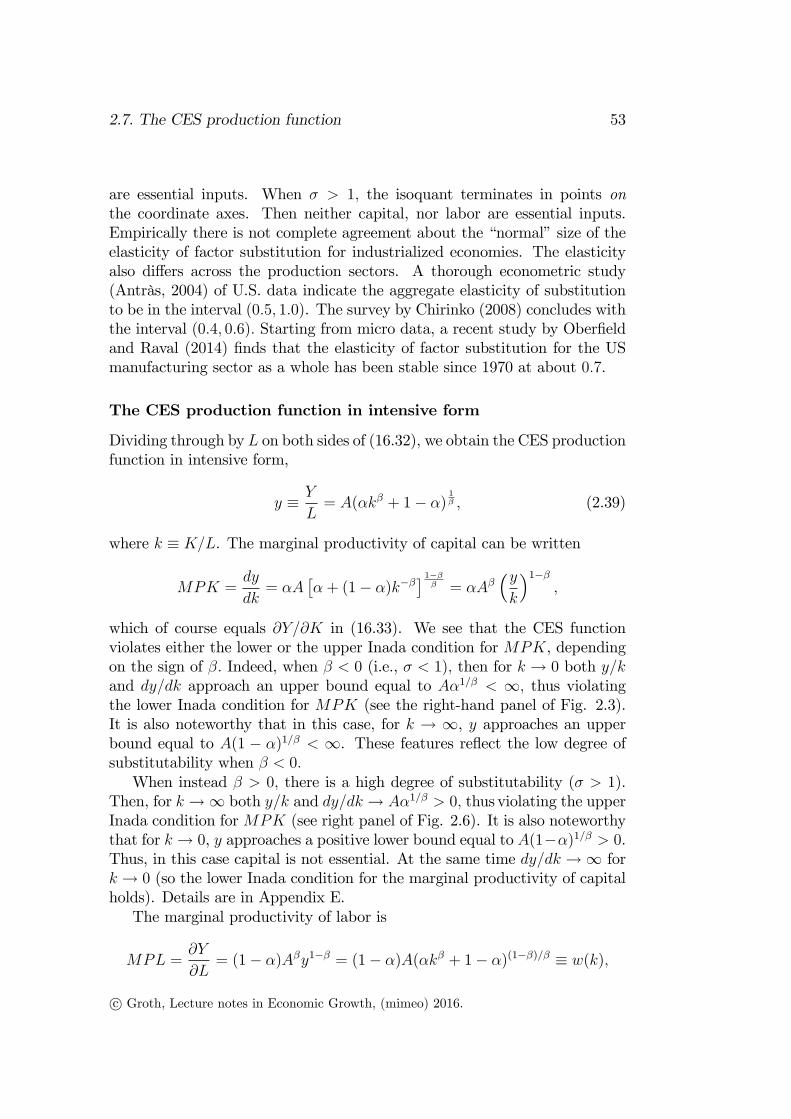
2.7. The CES production function 53
are essential inputs. When σ > 1, the isoquant terminates in points onthe coordinate axes. Then neither capital, nor labor are essential inputs.Empirically there is not complete agreement about the “normal”size of theelasticity of factor substitution for industrialized economies. The elasticityalso differs across the production sectors. A thorough econometric study(Antràs, 2004) of U.S. data indicate the aggregate elasticity of substitutionto be in the interval (0.5, 1.0). The survey by Chirinko (2008) concludes withthe interval (0.4, 0.6). Starting from micro data, a recent study by Oberfieldand Raval (2014) finds that the elasticity of factor substitution for the USmanufacturing sector as a whole has been stable since 1970 at about 0.7.
The CES production function in intensive form
Dividing through by L on both sides of (16.32), we obtain the CES productionfunction in intensive form,
y ≡ Y
L= A(αkβ + 1− α)
1β , (2.39)
where k ≡ K/L. The marginal productivity of capital can be written
MPK =dy
dk= αA
[α + (1− α)k−β
] 1−ββ = αAβ
(yk
)1−β,
which of course equals ∂Y/∂K in (16.33). We see that the CES functionviolates either the lower or the upper Inada condition for MPK, dependingon the sign of β. Indeed, when β < 0 (i.e., σ < 1), then for k → 0 both y/kand dy/dk approach an upper bound equal to Aα1/β < ∞, thus violatingthe lower Inada condition for MPK (see the right-hand panel of Fig. 2.3).It is also noteworthy that in this case, for k → ∞, y approaches an upperbound equal to A(1 − α)1/β < ∞. These features reflect the low degree ofsubstitutability when β < 0.When instead β > 0, there is a high degree of substitutability (σ > 1).
Then, for k →∞ both y/k and dy/dk → Aα1/β > 0, thus violating the upperInada condition forMPK (see right panel of Fig. 2.6). It is also noteworthythat for k → 0, y approaches a positive lower bound equal to A(1−α)1/β > 0.Thus, in this case capital is not essential. At the same time dy/dk →∞ fork → 0 (so the lower Inada condition for the marginal productivity of capitalholds). Details are in Appendix E.The marginal productivity of labor is
MPL =∂Y
∂L= (1− α)Aβy1−β = (1− α)A(αkβ + 1− α)(1−β)/β ≡ w(k),
c© Groth, Lecture notes in Economic Growth, (mimeo) 2016.
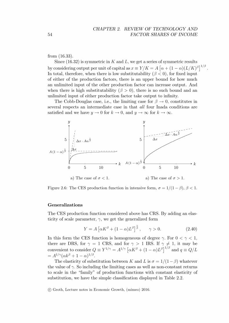
54CHAPTER 2. REVIEW OF TECHNOLOGY AND
FACTOR SHARES OF INCOME
from (16.33).Since (16.32) is symmetric inK and L, we get a series of symmetric results
by considering output per unit of capital as x≡ Y/K = A[α + (1− α)(L/K)β
]1/β.
In total, therefore, when there is low substitutability (β < 0), for fixed inputof either of the production factors, there is an upper bound for how muchan unlimited input of the other production factor can increase output. Andwhen there is high substitutability (β > 0), there is no such bound and anunlimited input of either production factor take output to infinity.The Cobb-Douglas case, i.e., the limiting case for β → 0, constitutes in
several respects an intermediate case in that all four Inada conditions aresatisfied and we have y → 0 for k → 0, and y →∞ for k →∞.
0 5 10
5
A (1 − α)1β
∆x ·Aα1β
∆x
a) The case of σ < 1.
k
y
0 5 10
5
A (1 − α)1β
∆x ·Aα1β
∆x
a) The case of σ > 1.
k
y
Figure 2.6: The CES production function in intensive form, σ = 1/(1− β), β < 1.
Generalizations
The CES production function considered above has CRS. By adding an elas-ticity of scale parameter, γ, we get the generalized form
Y = A[αKβ + (1− α)Lβ
] γβ , γ > 0. (2.40)
In this form the CES function is homogeneous of degree γ. For 0 < γ < 1,there are DRS, for γ = 1 CRS, and for γ > 1 IRS. If γ 6= 1, it may beconvenient to consider Q ≡ Y 1/γ = A1/γ
[αKβ + (1− α)Lβ
]1/βand q ≡ Q/L
= A1/γ(αkβ + 1− α)1/β.The elasticity of substitution between K and L is σ = 1/(1−β) whatever
the value of γ. So including the limiting cases as well as non-constant returnsto scale in the “family”of production functions with constant elasticity ofsubstitution, we have the simple classification displayed in Table 2.2.
c© Groth, Lecture notes in Economic Growth, (mimeo) 2016.
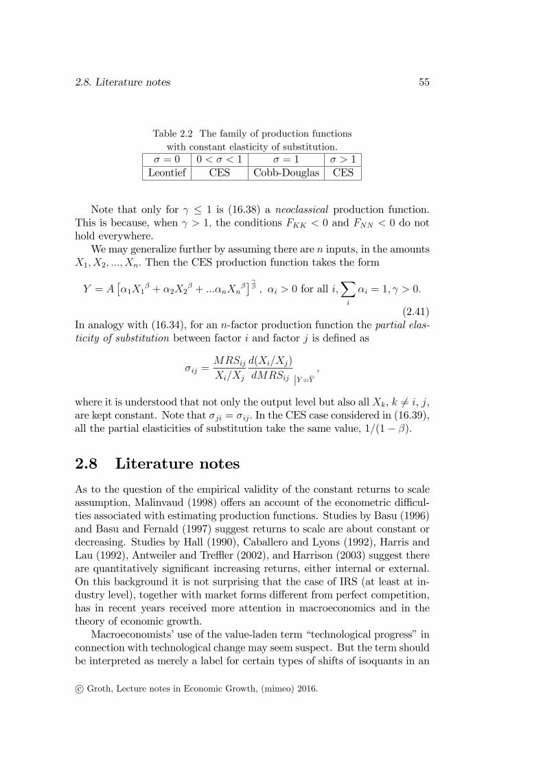
2.8. Literature notes 55
Table 2.2 The family of production functionswith constant elasticity of substitution.
σ = 0 0 < σ < 1 σ = 1 σ > 1Leontief CES Cobb-Douglas CES
Note that only for γ ≤ 1 is (16.38) a neoclassical production function.This is because, when γ > 1, the conditions FKK < 0 and FNN < 0 do nothold everywhere.We may generalize further by assuming there are n inputs, in the amounts
X1, X2, ..., Xn. Then the CES production function takes the form
Y = A[α1X1
β + α2X2β + ...αnXn
β] γβ , αi > 0 for all i,
∑i
αi = 1, γ > 0.
(2.41)In analogy with (16.34), for an n-factor production function the partial elas-ticity of substitution between factor i and factor j is defined as
σij =MRSijXi/Xj
d(Xi/Xj)
dMRSij |Y=Y
,
where it is understood that not only the output level but also all Xk, k 6= i, j,are kept constant. Note that σji = σij. In the CES case considered in (16.39),all the partial elasticities of substitution take the same value, 1/(1− β).
2.8 Literature notes
As to the question of the empirical validity of the constant returns to scaleassumption, Malinvaud (1998) offers an account of the econometric diffi cul-ties associated with estimating production functions. Studies by Basu (1996)and Basu and Fernald (1997) suggest returns to scale are about constant ordecreasing. Studies by Hall (1990), Caballero and Lyons (1992), Harris andLau (1992), Antweiler and Treffl er (2002), and Harrison (2003) suggest thereare quantitatively significant increasing returns, either internal or external.On this background it is not surprising that the case of IRS (at least at in-dustry level), together with market forms different from perfect competition,has in recent years received more attention in macroeconomics and in thetheory of economic growth.Macroeconomists’use of the value-laden term “technological progress”in
connection with technological change may seem suspect. But the term shouldbe interpreted as merely a label for certain types of shifts of isoquants in an
c© Groth, Lecture notes in Economic Growth, (mimeo) 2016.
56CHAPTER 2. REVIEW OF TECHNOLOGY AND
FACTOR SHARES OF INCOME
abstract universe. At a more concrete and disaggregate level analysts ofcourse make use of more refined notions about technological change, recog-nizing for example not only benefits of new technologies, but also the risks,including risk of fundamental mistakes (think of the introduction and laterabandonment of asbestos in the construction industry).Informative history of technology is contained in Ruttan (2001) and Smil
(2003). For more general economic history, see, e.g., Clark (2008) and Pers-son (2010). Forecasts of technological development in the next decades arecontained in, for instance, Brynjolfsson and McAfee (2014).Embodied technological progress, sometimes called investment-specific
technological progress, is explored in, for instance, Solow (1960), Greenwoodet al. (1997), and Groth and Wendner (2014). Hulten (2001) surveys theliterature and issues related to measurement of the direct contribution ofcapital accumulation and technological change, respectively, to productivitygrowth.Conditions ensuring that a representative household is admitted and the
concept of Gorman preferences are discussed in Acemoglu (2009). Anotheruseful source, also concerning the conditions for the representative firm to bea meaningful notion, is Mas-Colell et al. (1995). For general discussions of thelimitations of representative agent approaches, see Kirman (1992) and Galle-gati and Kirman (1999). Reviews of the “Cambridge Controversy”are con-tained in Mas-Colell (1989) and Felipe and Fisher (2003). The last-mentionedauthors find the conditions required for the well-behavedness of these con-structs so stringent that it is diffi cult to believe that actual economies arein any sense close to satisfy them. For a less distrustful view, see for in-stance Ferguson (1969), Johansen (1972), Malinvaud (1998), Jorgenson et al.(2005), and Jones (2005).It is often assumed that capital depreciation can be described as geomet-
ric (in continuous time exponential) evaporation of the capital stock. Thisformula is popular in macroeconomics, more so because of its simplicity thanits realism. An introduction to more general approaches to depreciation iscontained in, e.g., Nickell (1978).
2.9 References
(incomplete)Brynjolfsson, E., and A. McAfee, 2014, The Second Machine Age, Norton.Clark, G., 2008, A Farewell to Alms: A Brief Economic History of the
World, Princeton University Press.Persson, K. G., 2010, An economic history of Europe. Knowledge, insti-
c© Groth, Lecture notes in Economic Growth, (mimeo) 2016.
2.9. References 57
tutions and growth, 600 to the present, Cambridge University Press: Cam-bridge.Ruttan, V. W. , 2001, Technology, Growth, and Development: An Induced
Innovation Perspective, Oxford University Press: Oxford.Smil, V., 2003, Energy at the crossroads. Global perspectives and uncer-
tainties, MIT Press: Cambridge Mass.
c© Groth, Lecture notes in Economic Growth, (mimeo) 2016.
58CHAPTER 2. REVIEW OF TECHNOLOGY AND
FACTOR SHARES OF INCOME
c© Groth, Lecture notes in Economic Growth, (mimeo) 2016.
Chapter 3
Continuous time analysis
Because dynamic analysis is generally easier in continuous time, growth mod-
els are often stated in continuous time. This chapter gives an account of the
conceptual aspects of continuous time analysis. Appendix A considers sim-
ple growth arithmetic in continuous time. And Appendix B provides solution
formulas for linear first-order differential equations.
3.1 The transition from discrete time to con-
tinuous time
We start from a discrete time framework. The run of time is divided into
successive periods of equal length, taken as the time-unit. Let us here index
the periods by = 0 1 2 . Thus financial wealth accumulates according to
+1 − = 0 given,
where is (net) saving in period
3.1.1 Multiple compounding per year
With time flowing continuously, we let () refer to financial wealth at time
Similarly, (+∆) refers to financial wealth at time +∆ To begin with,
let ∆ equal one time unit. Then (∆) equals () and is of the same value
as Consider the forward first difference in ∆() ≡ (+∆)− () It
makes sense to consider this change in in relation to the length of the time
interval involved, that is, to consider the ratio ∆()∆ As long as ∆ = 1
with = ∆ we have ∆()∆ = (+1 − )1 = +1 − Now, keep
the time unit unchanged, but let the length of the time interval [ +∆)
59
60 CHAPTER 3. CONTINUOUS TIME ANALYSIS
approach zero, i.e., let ∆ → 0. When is a differentiable function of , we
have
lim∆→0
∆()
∆= lim
∆→0(+∆)− ()
∆=
()
where () often written () is known as the derivative of (·) at thepoint Wealth accumulation in continuous time can then be written
() = () (0) = 0 given, (3.1)
where () is the saving flow at time . For ∆ “small” we have the approx-
imation ∆() ≈ ()∆ = ()∆ In particular, for ∆ = 1 we have ∆()
= (+ 1)− () ≈ ()
As time unit choose one year. Going back to discrete time, if wealth
grows at a constant rate 0 per year, then after periods of length one
year, with annual compounding, we have
= 0(1 + ) = 0 1 2 . (3.2)
If instead compounding (adding saving to the principal) occurs times a
year, then after periods of length 1 year and a growth rate of per
such period,
= 0(1 +
) (3.3)
With still denoting time measured in years passed since date 0, we have
= periods. Substituting into (3.3) gives
() = = 0(1 +
) = 0
∙(1 +
1
)¸
where ≡
We keep and fixed, but let → ∞ Thus → ∞ Then, in the limit
there is continuous compounding and it can be shown that
() = 0 (3.4)
where is a mathematical constant called the base of the natural logarithm
and defined as ≡ lim→∞(1 + 1) ' 2.7182818285....The formula (3.4) is the continuous-time analogue to the discrete time
formula (3.2) with annual compounding. A geometric growth factor is re-
placed by an exponential growth factor, and this growth factor is valid
for any in the time interval (− 1 2) for which the growth rate of equalsthe constant (1 and 2 being some positive real numbers).
We can also view the formulas (3.2) and (3.4) as the solutions to a differ-
ence equation and a differential equation, respectively. Thus, (3.2) is the so-
lution to the linear difference equation +1 = (1+), given the initial value
c° Groth, Lecture notes in Economic Growth, (mimeo) 2016.
3.1. The transition from discrete time to continuous time 61
0 And (3.4) is the solution to the linear differential equation () = ()
given the initial condition (0) = 0 Now consider a time-dependent growth
rate, () The corresponding differential equation is () = ()() and it
has the solution
() = (0) 0() (3.5)
where the exponent,R 0() , is the definite integral of the function ()
from 0 to The result (3.5) is called the basic accumulation formula in
continuous time and the factor 0() is called the growth factor or the
accumulation factor.
3.1.2 Compound interest and discounting
Let () denote the short-term real interest rate in continuous time at time .
To clarify what is meant by this, consider a deposit of () euro on a drawing
account in a bank at time . If the general price level in the economy at time
is () euro, the real value of the deposit is () = () () at time
By definition the real rate of return on the deposit in continuous time (with
continuous compounding) at time is the (proportionate) instantaneous rate
at which the real value of the deposit expands per time unit when there is
no withdrawal from the account. Thus, if the instantaneous nominal interest
rate is () we have () () = () and so, by the fraction rule in continuous
time (cf. Appendix A),
() =()
()=
()
()− ()
()= ()− () (3.6)
where () ≡ () () is the instantaneous inflation rate. In contrast to the
corresponding formula in discrete time, this formula is exact. Sometimes ()
and () are referred to as the nominal and real interest intensity, respectively,
or the nominal and real force of interest.
Calculating the terminal value of the deposit at time 1 0 given its
value at time 0 and assuming no withdrawal in the time interval [0 1], the
accumulation formula (3.5) immediately yields
(1) = (0) 10
()
When calculating present values in continuous time analysis, we use com-
pound discounting. We reverse the accumulation formula and go from the
compounded or terminal value to the present value (0). Similarly, given a
consumption plan, (())1=0, the present value of this plan as seen from time
c° Groth, Lecture notes in Economic Growth, (mimeo) 2016.
62 CHAPTER 3. CONTINUOUS TIME ANALYSIS
0 is
=
Z 1
0
() − (3.7)
presupposing a constant interest rate. Instead of the geometric discount
factor, 1(1 + ) from discrete time analysis, we have here an exponential
discount factor, 1() = − and instead of a sum, an integral. When theinterest rate varies over time, (3.7) is replaced by
=
Z 1
0
() −
0()
In (3.7) () is discounted by − ≈ (1 + )− for “small”. This mightnot seem analogue to the discrete-time discounting in (??) where it is −1that is discounted by (1 + )− assuming a constant interest rate. Whentaking into account the timing convention that payment for −1 in period − 1 occurs at the end of the period (= time ) there is no discrepancy,
however, since the continuous-time analogue to this payment is ().
3.2 The allowed range for parameter values
The allowed range for parameters may change when we go from discrete time
to continuous time with continuous compounding. For example, the usual
equation for aggregate capital accumulation in continuous time is
() = ()− () (0) = 0 given, (3.8)
where () is the capital stock, () is the gross investment at time and
≥ 0 is the (physical) capital depreciation rate. Unlike in discrete time, here 1 is conceptually allowed. Indeed, suppose for simplicity that () = 0
for all ≥ 0; then (3.8) gives () = 0−. This formula is meaningful for
any ≥ 0 Usually, the time unit used in continuous time macro models isone year (or, in business cycle theory, rather a quarter of a year) and then a
realistic value of is of course 1 (say, between 0.05 and 0.10). However, if
the time unit applied to the model is large (think of a Diamond-style OLG
model), say 30 years, then 1 may fit better, empirically, if the model
is converted into continuous time with the same time unit. Suppose, for
example, that physical capital has a half-life of 10 years. With 30 years as
our time unit, inserting into the formula 12 = −3 gives = (ln 2) · 3 ' 2In many simple macromodels, where the level of aggregation is high, the
relative price of a unit of physical capital in terms of the consumption good
is 1 and thus constant. More generally, if we let the relative price of the
c° Groth, Lecture notes in Economic Growth, (mimeo) 2016.
3.3. Stocks and flows 63
capital good in terms of the consumption good at time be () and allow
() 6= 0 then we have to distinguish between the physical depreciation
of capital, and the economic depreciation, that is, the loss in economic
value of a machine per time unit. The economic depreciation will be () =
() − () namely the economic value of the physical wear and tear (and
technological obsolescence, say) minus the capital gain (positive or negative)
on the machine.
Other variables and parameters that by definition are bounded from below
in discrete time analysis, but not so in continuous time analysis, include rates
of return and discount rates in general.
3.3 Stocks and flows
An advantage of continuous time analysis is that it forces the analyst to make
a clear distinction between stocks (say wealth) and flows (say consumption
or saving). Recall, a stock variable is a variable measured as a quantity at a
given point in time. The variables () and () considered above are stock
variables. A flow variable is a variable measured as quantity per time unit
at a given point in time. The variables () () and () are flow variables.
One can not add a stock and a flow, because they have different de-
nominations. What is meant by this? The elementary measurement units
in economics are quantity units (so many machines of a certain kind or so
many liters of oil or so many units of payment, for instance) and time units
(months, quarters, years). On the basis of these elementary units we can form
composite measurement units. Thus, the capital stock, has the denomi-
nation “quantity of machines”, whereas investment, has the denomination
“quantity of machines per time unit” or, shorter, “quantity/time”. A growth
rate or interest rate has the denomination “(quantity/time)/quantity” =
“time−1”. If we change our time unit, say from quarters to years, the value
of a flow variable as well as a growth rate is changed, in this case quadrupled
(presupposing annual compounding).
In continuous time analysis expressions like()+() or()+() are
thus illegitimate. But one can write (+∆) ≈ ()+(()−())∆ or
()∆ ≈ (()− ())∆ In the same way, suppose a bath tub at time
contains 50 liters of water and that the tap pours 12liter per second into the
tub for some time. Then a sum like 50 + 12(/sec) does not make sense. But
the amount of water in the tub after one minute is meaningful. This amount
would be 50 + 12· 60 ((/sec)×sec) = 80 . In analogy, economic flow
variables in continuous time should be seen as intensities defined for every
in the time interval considered, say the time interval [0, ) or perhaps
c° Groth, Lecture notes in Economic Growth, (mimeo) 2016.
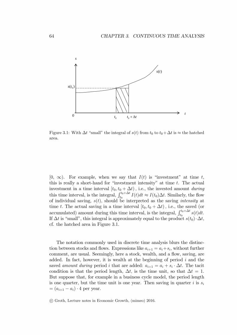
64 CHAPTER 3. CONTINUOUS TIME ANALYSIS
0 t
0( )s t
s
( )s t
0t 0t t
Figure 3.1: With ∆ “small” the integral of () from 0 to 0+∆ is ≈ the hatchedarea.
[0, ∞). For example, when we say that () is “investment” at time ,
this is really a short-hand for “investment intensity” at time . The actual
investment in a time interval [0 0 +∆) i.e., the invested amount during
this time interval, is the integral,R 0+∆
0() ≈ (0)∆ Similarly, the flow
of individual saving, () should be interpreted as the saving intensity at
time The actual saving in a time interval [0 0 +∆) i.e., the saved (or
accumulated) amount during this time interval, is the integral,R 0+∆
0()
If ∆ is “small”, this integral is approximately equal to the product (0) ·∆,
cf. the hatched area in Figure 3.1.
The notation commonly used in discrete time analysis blurs the distinc-
tion between stocks and flows. Expressions like +1 = + without further
comment, are usual. Seemingly, here a stock, wealth, and a flow, saving, are
added. In fact, however, it is wealth at the beginning of period and the
saved amount during period that are added: +1 = + ·∆. The tacit
condition is that the period length, ∆ is the time unit, so that ∆ = 1.
But suppose that, for example in a business cycle model, the period length
is one quarter, but the time unit is one year. Then saving in quarter is = (+1 − ) · 4 per year.
c° Groth, Lecture notes in Economic Growth, (mimeo) 2016.
3.4. The choice between discrete and continuous time formulation 65
3.4 The choice between discrete and contin-
uous time formulation
In empirical economics, data typically come in discrete time form and data
for flow variables typically refer to periods of constant length. One could
argue that this discrete form of the data speaks for discrete time rather than
continuous time modelling. And the fact that economic actors often think
and plan in period terms, may seem a good reason for putting at least mi-
croeconomic analysis in period terms. Nonetheless real time is continuous.
And, as for instance Allen (1967) argued, it can hardly be said that the
mass of economic actors think and plan with one and the same period. In
macroeconomics we consider the sum of the actions. In this perspective the
continuous time approach has the advantage of allowing variation within the
usually artificial periods in which the data are chopped up. And centralized
asset markets equilibrate very fast and respond immediately to new infor-
mation. For such markets a formulation in continuous time seems a better
approximation.
There is also a risk that a discrete time model may generate artificial
oscillations over time. Suppose the “true” model of some mechanism is given
by the differential equation
= −1 (3.9)
The solution is () = (0) which converges in a monotonic way toward 0
for →∞ However, the analyst takes a discrete time approach and sets up
the seemingly “corresponding” discrete time model
+1 − =
This yields the difference equation +1 = (1 + ), where 1 + 0 The
solution is = (1 + )0 = 0 1 2 As (1 + ) is positive when is
even and negative when is odd, oscillations arise (together with divergence
if −2) in spite of the “true” model generating monotonous convergencetowards the steady state ∗ = 0.It should be added, however, that this potential problem can always be
avoided within discrete time models by choosing a sufficiently short period
length. Indeed, the solution to a differential equation can always be ob-
tained as the limit of the solution to a corresponding difference equation for
the period length approaching zero. In the case of (3.9) the approximating
difference equation is +1 = (1 + ∆) where ∆ is the period length,
= ∆, and = (∆) By choosing ∆ small enough, the solution comes
c° Groth, Lecture notes in Economic Growth, (mimeo) 2016.
66 CHAPTER 3. CONTINUOUS TIME ANALYSIS
arbitrarily close to the solution of (3.9). It is generally more difficult to go
in the opposite direction and find a differential equation that approximates
a given difference equation. But the problem is solved as soon as a differ-
ential equation has been found that has the initial difference equation as an
approximating difference equation.
From the point of view of the economic contents, the choice between
discrete time and continuous time may be a matter of taste. Yet, everything
else equal, the clearer distinction between stocks and flows in continuous
time than in discrete time speaks for the former. From the point of view
of mathematical convenience, the continuous time formulation, which has
worked so well in the natural sciences, is preferable. At least this is so in
the absence of uncertainty. For problems where uncertainty is important,
discrete time formulations are easier to work with unless one is familiar with
stochastic calculus.
3.5 Appendix A: Growth arithmetic in con-
tinuous time
Let the variables and be differentiable functions of time Suppose
() () and () are positive for all Then:
PRODUCT RULE () = ()()⇒ ()
()=
()
()+
()
()
Proof. Taking logs on both sides of the equation () = ()() gives ln ()
= ln() + ln (). Differentiation w.r.t. , using the chain rule, gives the
conclusion. ¤
The procedure applied in this proof is called logarithmic differentiation
w.r.t.
FRACTION RULE () =()
()⇒ ()
()=
()
()− ()
()
The proof is similar.
POWER FUNCTION RULE () = () ⇒ ()
()=
()
()
The proof is similar.
In continuous time these simple formulas are exactly true. In discrete time
the analogue formulas are only approximately true and the approximation
can be quite bad unless the growth rates of and are small.
c° Groth, Lecture notes in Economic Growth, (mimeo) 2016.
3.6. Appendix B: Solution formulas for linear differential equations of first
order 67
3.6 Appendix B: Solution formulas for linear
differential equations of first order
For a general differential equation of first order, () = (() ) with
(0) = 0 and where is a continuous function, we have, at least for
in an interval (−+) for some 0
() = 0 +
Z
0
(() ) (*)
To get a confirmation, calculate () from (*).
For the special case of a linear differential equation of first order, () +
()() = () we can specify the solution. Three sub-cases of rising com-
plexity are:
1. () + () = with 6= 0 and initial condition (0) = 0 Solution:
() = (0 − ∗)−(−0) + ∗ where ∗ =
If = 0 we get, directly from (*), the solution () = 0 + 1
2. () + () = () with initial condition (0) = 0 Solution:
() = 0−(−0) + −(−0)
Z
0
()(−0)
Special case: () = with 6= − and initial condition (0) = 0
Solution:
() = 0−(−0)+−(−0)
Z
0
(+)(−0) = (0−
+ )−(−0)+
+ (−0)
3. () + ()() = () with initial condition (0) = 0 Solution:
() = 0−
0()
+ −
0()
Z
0
() 0()
1Some non-linear differential equations can be transformed into this simple case. For
simplicity let 0 = 0 Consider the equation () = () 0 0 given, 6= 0 6= 1
(a Bernoulli equation). To find the solution for () let () ≡ ()1− Then, ()= (1 − )()− () = (1 − )()−() = (1 − ) The solution for this is ()
= 0 + (1 − ) where 0 = 1−0 Thereby the solution for () is () = ()1(1−)
=³1−0 + (1− )
´1(1−) which is defined for −1−0 ((1− )
c° Groth, Lecture notes in Economic Growth, (mimeo) 2016.
68 CHAPTER 3. CONTINUOUS TIME ANALYSIS
Special case: () = 0 Solution:
() = 0−
0()
Even more special case: () = 0 and () = a constant. Solution:
() = 0−(−0)
Remark 1 For 0 = 0 most of the formulas will look simpler.
Remark 2 To check whether a suggested solution is a solution, calculate
the time derivative of the suggested solution and add an arbitrary constant.
By appropriate adjustment of the constant, the final result should be a repli-
cation of the original differential equation together with its initial condition.
c° Groth, Lecture notes in Economic Growth, (mimeo) 2016.
Chapter 4
Skill-biased technical change.
Balanced growth theorems
This chapter is both an alternative and a supplement to the pages 60-64
in Acemoglu, where the concepts of neutral technical change and balanced
growth, including Uzawa’s theorem, are discussed.
Since “neutral” technical change should be seen in relation to “biased”
technical change, Section 1 below introduces the concept of “biased” tech-
nical change. Also concerning biased technical change do three different
definitions, Hicks’, Harrod’s, and what the literature has dubbed “Solow’s”.
Below we concentrate on Hick’s definition − with an application to how tech-nical change affects the evolution of the skill premium. So the focus is on the
production factors skilled and unskilled labor rather than capital and labor.
While regarding capital and labor it is Harrod’s classifications that are most
used in macroeconomics, regarding skilled and unskilled labor it is Hicks’.
The remaining sections discuss the concept of balanced growth and present
three fundamental propositions about balanced growth. In view of the gen-
erality of the propositions, they have a broad field of application. Our propo-
sitions 1 and 2 are slight extensions of part 1 and 2, respectively, of what
Acemoglu calls Uzawa’s Theorem I (Acemoglu, 2009, p. 60). Our Proposi-
tion 3 essentially corresponds to what Acemoglu calls Uzawa’s Theorem II
(Acemoglu, 2009, p. 63).
69
70
CHAPTER 4. SKILL-BIASED TECHNICAL CHANGE.
BALANCED GROWTH THEOREMS
4.1 The rising skill premium
4.1.1 Skill-biased technical change in the sense of Hicks:
An example
Let aggregate output be produced through a differentiable three-factor pro-
duction function :
= (1 2 )
where is capital input, 1 is input of unskilled labor (also called blue-collar
labor below), and 2 is input of skilled labor. Suppose technological change
is such that the production function can be rewritten
(1 2 ) = ((1 2 )) (4.1)
where the “nested” function (1 2 ) represents input of a “human cap-
ital” aggregate. Let be CRS-neoclassical w.r.t. and and let
be CRS-neoclassical w.r.t. (1 2) Finally, let 0. So “technical
change” amounts to “technical progress”.
In equilibrium under perfect competition in the labor markets the relative
wage, often called the “skill premium”, will be
2
1=
2
1=
2
1=
2(1 2 )
1(1 2 )=
2(1 21 )
1(1 21 ) (4.2)
where we have used Euler’s theorem (saying that if is homogeneous of
degree one in its first two arguments, then the partial derivatives of are
homogeneous of degree zero w.r.t. these arguments).
Time is continuous (nevertheless the time argument of a variable, is in
this section written as a subscript ). Hicks’ definitions are now: If for all
21 0
³2(121)
1(121)
´
21
constantT 0 then technical change is⎧⎨⎩ skill-biased in the sense of Hicks,
skill-neutral in the sense of Hicks.
blue collar-biased in the sense of Hicks,
(4.3)
respectively.
In the US the skill premium (measured by the wage ratio for college
grads vis-a-vis high school grads) has had an upward trend since 1950 (see
c° Groth, Lecture notes in Economic Growth, (mimeo) 2016.
4.1. The rising skill premium 71
for instance Jones and Romer, 2010).1 If in the same period the relative
supply of skilled labor had been roughly constant, by (4.3) in combination
with (4.2), a possible explanation could be that technological change has
been skill-biased in the sense of Hicks. In reality, in the same period also the
relative supply of skilled labor has been rising (in fact even faster than the
skill premium). Since in spite of this the skill premium has risen, it suggests
that the extend of “skill-biasedness” has been even stronger.
Wemay alternatively put it this way. As the function is CRS-neoclassical
w.r.t. 1 and 2 we have 22 0 and 12 0 cf. Chapter 2. Hence, by
(4.2), a rising 21 without technical change would imply a declining skill
premium. That the opposite has happened must, within our simple model,
be due to (a) there has been technical change, and (b) technical change
has favoured skilled labor (which means that technical change has been skill-
biased in the sense of Hicks).
An additional aspect of the story is that skill-biasedness helps explain
the observed increase in the relative supply of skilled labor. If for a constant
relative supply of skilled labor, the skill premium is increasing, this increase
strengthens the incentive to go to college. Thereby the relative supply of
skilled labor (reflecting the fraction of skilled labor in the labor force) tends
to increase.
4.1.2 Capital-skill complementarity
An additional potential source of a rising skill premium is capital-skill com-
plementarity. Let the aggregate production function be
= (1 2 ) = (11 22) = (+11)(22)
1− 0 1
where 1 and 2 are technical coefficients that may be rising over time.
In this production function capital and unskilled labor are perfectly substi-
tutable (the partial elasticity of factor substitution between them is +∞) Onthe other hand there is direct complementarity between capital and skilled
labor, i.e., 2(2) 0
Under perfect competition the skill premium is
2
1=
2
2=( +11)
(1− )(22)−2
( +11)−11(22)1−(4.4)
=1−
µ +11
22
¶2
1
1On the other hand, over the years 1915 - 1950 the skill premium had a downward
trend (Jones and Romer, 2010).
c° Groth, Lecture notes in Economic Growth, (mimeo) 2016.
72
CHAPTER 4. SKILL-BIASED TECHNICAL CHANGE.
BALANCED GROWTH THEOREMS
Here, if technical change is absent (1 and 2 constant), a rising capital
stock will, for fixed 1 and 2 raise the skill premium.
A more realistic scenario is, however, a situation with an approximately
constant real interest rate, cf. Kaldor’s stylized facts. We have, again by
perfect competition,
= ( +11)
−1(22)1− =
µ +11
22
¶−1= + (4.5)
where is the real interest rate at time and is the (constant) capital
depreciation rate. For = a constant, (4.5) gives
+11
22=
µ +
¶− 11−≡ (4.6)
a constant. In this case, (4.4) shows that capital-skill complementarity is
not sufficient for a rising skill premium. A rising skill premium requires that
technical change brings about a rising 21. So again an observed rising
skill premium, along with a more or less constant real interest rate, suggests
that technical change is skill-biased.
We may rewrite (4.6) as
22= − 11
22
where the conjecture is that 11(22) → 0 for → ∞ The analysis
suggests the following story. Skill-biased technical progress generates rising
productivity as well as a rising skill premium. The latter induces more and
more people to go to college. The rising level of education in the labor force
raises productivity further. This is a basis for further capital accumulation,
continuing to replace unskilled labor, and so on.
In particular since the early 1980s the skill premium has been sharply
increasing in the US (see Acemoglu, p. 498). This is also the period where
ICT technologies took off.
4.2 Balanced growth and constancy of key ra-
tios
The focus now shifts to homogeneous labor vis-a-vis capital.
We shall state general definitions of the concepts of “steady state” and
“balanced growth”, concepts that are related but not identical. With respect
c° Groth, Lecture notes in Economic Growth, (mimeo) 2016.
4.2. Balanced growth and constancy of key ratios 73
to “balanced growth” this implies a minor deviation from the way Acemoglu
briefly defines it informally on his page 57. The main purpose of the present
chapter is to lay bare the connections between these two concepts as well
as their relation to the hypothesis of Harrod-neutral technical progress and
Kaldor’s stylized facts.
4.2.1 The concepts of steady state and balanced growth
A basic equation in many one-sector growth models for a closed economy in
continuous time is
= − = − − ≡ − (4.7)
where is aggregate capital, aggregate gross investment, aggregate
output, aggregate consumption, aggregate gross saving (≡ −), and
≥ 0 is a constant physical capital depreciation rate.Usually, in the theoretical literature on dynamic models, a steady state is
defined in the following way:
Definition 3 A steady state of a dynamic model is a stationary solution to
the fundamental differential equation(s) of the model.
Or briefly: a steady state is a stationary point of a dynamic process.
Let us take the Solow growth model as an example. Here gross saving
equals where is a constant, 0 1 Aggregate output is given by a
neoclassical production function, with CRS and Harrod-neutral technical
progress: = () = ( 1) ≡ () where is the labor
force, is the level of technology, and ≡ () is the (effective) capital
intensity. Moreover, 0 0 and 00 0 Solow assumes () = (0) and
() = (0), where and ≥ 0 are the constant growth rates of the laborforce and technology, respectively. By log-differentiating w.r.t. 2 we end
up with the fundamental differential equation (“law of motion”) of the Solow
model: · = ()− ( + + ) (4.8)
Thus, in the Solow model, a (non-trivial) steady state is a ∗ 0 such that,
if = ∗ then· = 0 In passing we note that, by (4.8), such a ∗ must
satisfy the equation (∗)∗ = ( + + ) and in view of 00 0 it is
unique and globally asymptotically stable if it exists. A sufficient condition
2Or by directly using the fraction rule, see Appendix A to Chapter 3.
c° Groth, Lecture notes in Economic Growth, (mimeo) 2016.
74
CHAPTER 4. SKILL-BIASED TECHNICAL CHANGE.
BALANCED GROWTH THEOREMS
for its existence is that + + 0 and satisfies the Inada conditions
lim→0 0() =∞ and lim→∞ 0() = 0
The most common definition in the literature of balanced growth for an
aggregate economy is the following:
Definition 4 A balanced growth path is a path ()∞=0 along which thequantities and are positive and grow at constant rates (not necessarily
positive and not necessarily the same).
Acemoglu, however, defines (Acemoglu, 2009, p. 57) balanced growth
in the following way: “balanced growth refers to an allocation where output
grows at a constant rate and capital-output ratio, the interest rate, and factor
shares remain constant”. My problem with this definition is that it mixes
growth of aggregate quantities with income distribution aspects (interest rate
and factor income shares). And it is not made clear what is meant by the
output-capital ratio if the relative price of capital goods is changing over
time. So I stick to the definition above which is quite standard and is known
to function well in many different contexts.
Note that in the Solow model (as well as in many other models) we have
that if the economy is in a steady state, = ∗ then the economy featuresbalanced growth. Indeed, a steady state of the Solow model implies by
definition that ≡ () is constant. Hence must grow at the same
constant rate as namely + In addition, = (∗) in a steadystate, showing that also must grow at the constant rate + And so
must then = (1 − ) So in a steady state of the Solow model the path
followed by ()∞=0 is a balanced growth path.As we shall see in the next section, in the Solow model (and many other
models) the reverse also holds: if the economy features balanced growth,
then it is in a steady state. But this equivalence between steady state and
balanced growth does not hold in all models.
4.2.2 A general result about balanced growth
An interesting fact is that, given the dynamic resource constraint (4.7), we
have always that if there is balanced growth with positive gross saving, then
the ratios and are constant (by “always” is meant: independently
of how saving is determined and how the labor force and technology evolve).
And also the other way round: as long as gross saving is positive, constancy of
the and ratios is enough to ensure balanced growth. So balanced
growth and constancy of certain key ratios are essentially equivalent.
This is a very practical general observation. And since Acemoglu does not
state any balanced growth theorem at this general level, we shall do it here,
c° Groth, Lecture notes in Economic Growth, (mimeo) 2016.
4.2. Balanced growth and constancy of key ratios 75
together with a proof. Letting denote the growth rate of the (positively
valued) variable i.e., ≡ we claim:
Proposition 1 (the balanced growth equivalence theorem). Let ()∞=0be a path along which , and ≡ − are positive for all ≥ 0Then, given the accumulation equation (4.7), the following holds:
(i) if there is balanced growth, then = = and the ratios
and are constant;
(ii) if and are constant, then and grow at the same
constant rate, i.e., not only is there balanced growth, but the growth
rates of and are the same.
Proof Consider a path ()∞=0 along which , and ≡ −
are positive for all ≥ 0 (i) Assume there is balanced growth. Then, by
definition, and are constant. Hence, by (4.7), we have that =
+ is constant, implying
= (*)
Further, since = +
=
=
+
=
+
=
+
(by (*))
=
+
−
=
( − ) + (**)
Now, let us provisionally assume that 6= Then (**) gives
=
−
− (***)
which is a constant since and are constant. Constancy of
requires that = hence, by (***), = 1 i.e., = In view
of = + , however, this outcome contradicts the given condition that
0 Hence, our provisional assumption and its implication, (***), are
falsified. Instead we have = . By (**), this implies = = but
now without the condition = 1 being implied. It follows that and
are constant.
(ii) Suppose and are constant. Then = = , so that
is a constant. We now show that this implies that is constant.
Indeed, from (4.7), = 1− so that also is constant. It follows
that = = so that is constant. By (4.7),
=
+
= +
c° Groth, Lecture notes in Economic Growth, (mimeo) 2016.
76
CHAPTER 4. SKILL-BIASED TECHNICAL CHANGE.
BALANCED GROWTH THEOREMS
so that is constant. This, together with constancy of and
implies that also and are constant. ¤
Remark. It is part (i) of the proposition which requires the assumption 0
for all ≥ 0 If = 0 we would have = − and ≡ − = hence
= for all ≥ 0 Then there would be balanced growth if the commonvalue of and had a constant growth rate. This growth rate, however,
could easily differ from that of Suppose = 1− = and =
( and constants). Then we would have = = −+(1−) whichcould easily be strictly positive and thereby different from = − ≤ 0 sothat (i) no longer holds. ¤
The nice feature is that this proposition holds for any model for which
the simple dynamic resource constraint (4.7) is valid. No assumptions about
for example CRS and other technology aspects or about market form are
involved. Note also that Proposition 1 suggests a link from balanced growth
to steady state. And such a link is present in for instance the Solow model.
Indeed, by (i) of Proposition 1, balanced growth implies constancy of
which in the Solow model implies that () is constant. In turn, the latter
is only possible if is constant, that is, if the economy is in steady state.
There exist cases, however, where this equivalence does not hold (some
open economy models and some models with embodied technological change,
see Groth et al., 2010). Therefore, it is recommendable always to maintain
a distinction between the terms steady state and balanced growth.
4.3 The crucial role of Harrod-neutrality
Proposition 1 suggests that if one accepts Kaldor’s stylized facts (see Chapter
1) as a characterization of the past century’s growth experience, and if one
wants a model consistent with them, one should construct the model such
that it can generate balanced growth. For a model to be capable of generating
balanced growth, however, technological progress must be of the Harrod-
neutral type (i.e., be labor-augmenting), at least in a neighborhood of the
balanced growth path. For a fairly general context (but of course not as
general as that of Proposition 1), this was shown already by Uzawa (1961).
We now present a modernized version of Uzawa’s contribution.
Let the aggregate production function be
() = (() () ) 0 (4.9)
where is a constant that depends on measurement units. The only tech-
nology assumption needed is that has CRS w.r.t. the first two arguments
c° Groth, Lecture notes in Economic Growth, (mimeo) 2016.
4.3. The crucial role of Harrod-neutrality 77
( need not be neoclassical for example). As a representation of technical
progress, we assume 0 for all ≥ 0 (i.e., as time proceeds, un-
changed inputs result in more and more output). We also assume that the
labor force evolves according to
() = (0) (4.10)
where is a constant. Further, non-consumed output is invested and so (4.7)
is the dynamic resource constraint of the economy.
Proposition 2 (Uzawa’s balanced growth theorem) Let = ( () () ())∞=0,where 0 () () for all ≥ 0 be a path satisfying the capital accumu-lation equation (4.7), given the CRS-production function (4.9) and the labor
force path in (4.10). Then:
(i) a necessary condition for this path to be a balanced growth path is that
along the path it holds that
() = (() () ) = (() ()() 0) (4.11)
where () = with ≡ − ;
(ii) for any 0 such that there is a + + with the property that
the production function in (4.9) allows an output-capital ratio equal
to at = 0 (i.e., (1 −1 0) = for some real number 0), a
sufficient condition for to be compatible with a balanced growth path
with output-capital ratio , is that can be written as in (4.11) with
() = .
Proof (i)3 Suppose the path ( ()() ())∞=0 is a balanced growth path.By definition, and are then constant, so that () = (0) and
() = (0) We then have
()− = (0) = ((0) (0) 0) = (()− ()− 0) (*)
where we have used (4.9) with = 0 In view of the precondition that ()
≡ ()−() 0 we know from (i) of Proposition 1, that is constant
so that = . By CRS, (*) then implies
() = (() − () − 0) = (() ( −)() 0)
3This part draws upon Schlicht (2006), who generalized a proof in Wan (1971, p. 59)
for the special case of a constant saving rate.
c° Groth, Lecture notes in Economic Growth, (mimeo) 2016.
78
CHAPTER 4. SKILL-BIASED TECHNICAL CHANGE.
BALANCED GROWTH THEOREMS
We see that (4.11) holds for () = with ≡ −
(ii) Suppose (4.11) holds with () = Let ≥ 0 be given such thatthere is a + + 0 with the property that
(1 −1 0) = (**)
for some constant 0 Our strategy is to prove the claim in (ii) by con-
struction of a path = ( ()() ())∞=0 which satisfies it. We let be
such that the saving-income ratio is a constant ≡ (++) ∈ (0 1), i.e., ()−() ≡ () = () for all ≥ 0 Inserting this, together with () =(())()(), where (()) ≡ (() 1 0) and () ≡ ()(()())
into (4.7), rearranging gives the Solow equation (4.8). Hence () is con-
stant if and only if () satisfies the equation (())() = ( + + )
≡ By (**) and the definition of the required value of () is which
is consequently the unique steady state for the constructed Solow equa-
tion. Letting (0) satisfy (0) = (0) where = (0) we thus have
(0) = (0)((0)(0)) = So that the initial value of () equals the
steady state value. It follows that () = for all ≥ 0 and so ()()= (())() = () = for all ≥ 0 In addition, () = (1− ) ()
so that () () is constant along the path As both and are
thus constant along the path by (ii) of Proposition 1 follows that is a
balanced growth path, as was to be proved. ¤
The form (4.11) indicates that along a balanced growth path, technical
progress must be purely “labor augmenting”, that is, Harrod-neutral. It is in
this case convenient to define a new CRS function, by (() ()())
≡ (() ()() 0) Then (i) of the proposition implies that at least along
the balanced growth path, we can rewrite the production function this way:
() = (() (0)() ) = (() ()()) (4.12)
where (0) = and () = (0) with ≡ −
It is important to recognize that the occurrence of Harrod-neutrality says
nothing about what the source of technological progress is. Harrod-neutrality
should not be interpreted as indicating that the technological progress em-
anates specifically from the labor input. Harrod-neutrality only means that
technical innovations predominantly are such that not only do labor and cap-
ital in combination become more productive, but this happens to manifest
itself at the aggregate level in the form (4.12).4
4For a CRS Cobb-Douglas production function with technological progress, Harrod-
neutrality is present whenever the output elasticity w.r.t capital (often denoted ) is
constant over time.
c° Groth, Lecture notes in Economic Growth, (mimeo) 2016.
4.3. The crucial role of Harrod-neutrality 79
What is the intuition behind the Uzawa result that for balanced growth to
be possible, technical progress must have the purely labor-augmenting form?
First, notice that there is an asymmetry between capital and labor. Capital
is an accumulated amount of non-consumed output. In contrast, in simple
macro models labor is a non-produced production factor which (at least in
the context of (4.10)) grows in an exogenous way. Second, because of CRS,
the original formulation, (4.9), of the production function implies that
1 = (()
()()
() ) (4.13)
Now, since capital is accumulated non-consumed output, it tends to inherit
the trend in output such that () () must be constant along a balanced
growth path (this is what Proposition 1 is about). Labor does not inherit the
trend in output; indeed, the ratio () () is free to adjust as time proceeds.
When there is technical progress ( 0) along a balanced growth path,
this progress must manifest itself in the form of a changing () () in (13.5)
as proceeds, precisely because () () must be constant along the path.
In the “normal” case where 0 the needed change in () () is a
fall (i.e., a rise in ()()) This is what (13.5) shows. Indeed, the fall in
() () must exactly offset the effect on of the rising when there is a
fixed capital-output ratio.5 It follows that along the balanced growth path,
()() is an increasing implicit function of If we denote this function
() we end up with (4.12) with specified properties (given by and ).
The generality of Uzawa’s theorem is noteworthy. The theorem assumes
CRS, but does not presuppose that the technology is neoclassical, not to
speak of satisfying the Inada conditions.6 And the theorem holds for exoge-
nous as well as endogenous technological progress. It is also worth mentioning
that the proof of the sufficiency part of the theorem is constructive. It pro-
vides a method to construct a hypothetical balanced growth path (BGP from
now).7
A simple implication of the Uzawa theorem is the following. Interpreting
the () in (4.11) as the “level of technology”, we have:
COROLLARY Along a BGP with positive gross saving and the technology
level, () growing at the rate ≥ 0 output grows at the rate + while
labor productivity, ≡ and consumption per unit of labor, ≡
grow at the rate
5This way of presenting the intuition behind the Uzawa result draws upon Jones and
Scrimgeour (2008).6Many accounts of the Uzawa theorem, including Jones and Scrimgeour (2008), presume
a neoclassical production function, but the theorem is much more general.7Part (ii) of Proposition 2 is left out in Acemoglu’s book.
c° Groth, Lecture notes in Economic Growth, (mimeo) 2016.
80
CHAPTER 4. SKILL-BIASED TECHNICAL CHANGE.
BALANCED GROWTH THEOREMS
Proof That = + follows from (i) of Proposition 2. As to the growth
rate of labor productivity we have
= (0)
(0)= (0)( −) = (0)
Finally, by Proposition 1, along a BGP with 0 ≡ must grow at
the same rate as ¤We shall now consider the implication of Harrod-neutrality for the income
shares of capital and labor when the technology is neoclassical and markets
are perfectly competitive.
4.4 Harrod-neutrality and the functional in-
come distribution
There is one facet of Kaldor’s stylized facts we have so far not related to
Harrod-neutral technical progress, namely the long-run “approximate” con-
stancy of both the income share of labor, and the rate of return to
capital. At least with neoclassical technology, profit maximizing firms, and
perfect competition in the output and factor markets, these properties are
inherent in the combination of constant returns to scale, balanced growth,
and the assumption that the relative price of capital goods (relative to con-
sumption goods) is constant over time. The latter condition holds in models
where the capital good is nothing but non-consumed output, cf. (4.7).8
To see this, we start out from a neoclassical CRS production function
with Harrod-neutral technological progress,
() = (() ()()) (4.14)
With () denoting the real wage at time in equilibrium under perfect
competition the labor income share will be
()()
()=
()
()()
()=
2(() ()())()()
() (4.15)
In this simple model, without natural resources, (gross) capital income equals
non-labor income, () − ()() Hence, if () denotes the (net) rate of
return to capital at time , then
() = ()− ()()− ()
() (4.16)
8The reader may think of the “corn economy” example in Acemoglu, p. 28.
c° Groth, Lecture notes in Economic Growth, (mimeo) 2016.
4.4. Harrod-neutrality and the functional income distribution 81
Denoting the (gross) capital income share by () we can write this ()
(in equilibrium) in three ways:
() ≡ ()− ()()
()=(() + )()
()
() = (() ()())− 2(() ()())()()
()=
1(() ()())()
()
() =
()
()()
() (4.17)
where the first row comes from (4.16), the second from (4.14) and (4.15), the
third from the second together with Euler’s theorem.9 Comparing the first
and the last row, we see that in equilibrium
()
()= () +
In this condition we recognize one of the first-order conditions in the rep-
resentative firm’s profit maximization problem under perfect competition,
since () + can be seen as the firm’s required gross rate of return.10
In the absence of uncertainty, the equilibrium real interest rate in the
bond market must equal the rate of return on capital, () And () + can
then be seen as the firm’s cost of disposal over capital per unit of capital per
time unit, consisting of interest cost plus capital depreciation.
Proposition 3 (factor income shares and rate of return under balanced
growth) Let the path (() () ())∞=0 be a BGP in a competitive economywith the production function (4.14) and with positive saving. Then, along the
BGP, the () in (4.17) is a constant, ∈ (0 1). The labor income sharewill be 1− and the (net) rate of return on capital will be = − where
is the constant output-capital ratio along the BGP.
Proof By CRS we have () = (() ()()) = ()() (() 1)
≡ ()()(()) In view of part (i) of Proposition 2, by balanced growth,
()() is some constant, . Since ()() = (())() and 00 0this implies () constant, say equal to ∗ But ()() = 0(()) which
9From Euler’s theorem, 1 + 2 = () when is homogeneous of degree
one10With natural resources, say land, entering the set of production factors, the formula,
(4.16), for the rate of return to capital should be modified by subtracting land rents from
the numerator.
c° Groth, Lecture notes in Economic Growth, (mimeo) 2016.
82
CHAPTER 4. SKILL-BIASED TECHNICAL CHANGE.
BALANCED GROWTH THEOREMS
then equals the constant 0(∗) along the BGP. It then follows from (4.17)
that () = 0(∗) ≡ Moreover, 0 1 where 0 follows from
0 0 and 1 from the fact that = = (∗)∗ 0(∗) in viewof 00 0 and (0) ≥ 0 Then, by the first equality in (4.17), ()() ()= 1− () = 1− . Finally, by (4.16), the (net) rate of return on capital is
= (1− ()() ()) ()()− = − ¤
This proposition is of interest by displaying a link from balanced growth
to constancy of factor income shares and the rate of return, that is, some
of the “stylized facts” claimed by Kaldor. Note, however, that although the
proposition implies constancy of the income shares and the rate of return,
it does not determine them, except in terms of and But both and,
generally, are endogenous and depend on ∗11 which will generally beunknown as long as we have not specified a theory of saving. This takes us
to theories of aggregate saving, for example the simple Ramsey model, cf.
Chapter 8 in Acemoglu’s book.
4.5 What if technological change is embod-
ied?
In our presentation of technological progress above we have implicitly as-
sumed that all technological change is disembodied. And the way the propo-
sitions 1, 2, and 3, are formulated assume this.
As noted in Chapter 2, disembodied technological change occurs when new
technical knowledge advances the combined productivity of capital and labor
independently of whether the workers operate old or new machines. Consider
again the aggregate dynamic resource constraint (4.7) and the production
function (4.9):
() = ()− () (4.18)
() = (() () ) 0 (4.19)
Here ()−() is aggregate gross investment, () For a given level of ()the resulting amount of new capital goods per time unit (()+()), mea-
sured in efficiency units, is independent of when this investment occurs. It is
thereby not affected by technological progress. Similarly, the interpretation
of 0 in (4.19) is that the higher technology level obtained as time
proceeds results in higher productivity of all capital and labor. Thus also
11As to there is of course a trivial exception, namely the case where the production
function is Cobb-Douglas and therefore is a given parameter.
c° Groth, Lecture notes in Economic Growth, (mimeo) 2016.
4.5. What if technological change is embodied? 83
firms that have only old capital equipment benefit from recent advances in
technical knowledge. No new investment is needed to take advantage of the
recent technological and organizational developments.12
In contrast, we say that technological change is embodied, if taking ad-
vantage of new technical knowledge requires construction of new investment
goods. The newest technology is incorporated in the design of newly pro-
duced equipment; and this equipment will not participate in subsequent
technological progress. Whatever the source of new technical knowledge,
investment becomes an important bearer of the productivity increases which
this new knowledge makes possible. Without new investment, the potential
productivity increases remain potential instead of being realized.
As also noted in Chapter 2, we may represent embodied technological
progress by writing capital accumulation in the following way,
() = ()()− () (4.20)
where () is gross investment at time and () measures the “quality”
(productivity) of newly produced investment goods. The increasing level of
technology implies increasing () so that a given level of investment gives
rise to a greater and greater additions to the capital stock, measured
in efficiency units. As in our aggregate framework, capital goods can be
produced at the same minimum cost as one consumption good, we have · =1 where is the equilibrium price of capital goods in terms of consumption
goods. So embodied technological progress is likely to result in a steady
decline in the relative price of capital equipment, a prediction confirmed by
the data (see, e.g., Greenwood et al., 1997).
This raises the question how the propositions 1, 2, and 3 fare in the case
of embodied technological progress. The answer is that a generalized version
of Proposition 1 goes through. Essentially, we only need to replace (4.7) by
(13.13) and interpret in Proposition 1 as the value of the capital stock,
i.e., we have to replace by =
But the concept of Harrod-neutrality no longer fits the situation with-
out further elaboration. Hence to obtain analogies to Proposition 2 and
Proposition 3 is a more complicated matter. Suffice it to say that with em-
bodied technological progress, the class of production functions that are con-
sistent with balanced growth is smaller than with disembodied technological
progress.
12In the standard versions of the Solow model and the Ramsey model it is assumed that
all technological progress has this form - for no other reason than that this is by far the
simplest case to analyze.
c° Groth, Lecture notes in Economic Growth, (mimeo) 2016.
84
CHAPTER 4. SKILL-BIASED TECHNICAL CHANGE.
BALANCED GROWTH THEOREMS
4.6 Concluding remarks
In the Solow model as well as in many other models with disembodied techno-
logical progress, a steady state and a balanced growth path imply each other.
Indeed, they are in that model, as well as many others, two sides of the same
process. There exist exceptions, however, that is, cases where steady state
and a balanced growth are not equivalent (some open economy models and
some models with embodied technical change). So the two concepts should
be held apart.13
Note that the definition of balanced growth refers to aggregate variables.
At the same time as there is balanced growth at the aggregate level, structural
change may occur. That is, a changing sectorial composition of the economy
is under certain conditions compatible with balanced growth (in a generalized
sense) at the aggregate level, cf. the “Kuznets facts” (see Kongsamut et al.,
2001, and Acemoglu, 2009, Chapter 20).
In view of the key importance of Harrod-neutrality, a natural question is:
has growth theory uncovered any endogenous tendency for technical progress
to converge to Harrod-neutrality? Fortunately, in his Chapter 15 Acemoglu
outlines a theory about a mechanism entailing such a tendency, the theory of
“directed technical change”. Jones (2005) suggests an alternative mechanism.
4.7 References
Acemoglu, D., 2009, Introduction to Modern Economic Growth, Princeton
University Press: Oxford.
Barro, R., and X. Sala-i-Martin, 2004, Economic Growth, second edition,
MIT Press: Cambridge (Mass.)
Duffy. J., C. Papageorgiou, and F. Perez-Sebastian, 2004, Capital-Skill
Complementarity? Evidence from a Panel of Countries, The Review of
Economics and Statistics, vol. 86(1), 327-344.
Gordon, R. J., 1990. The Measurement of Durable goods Prices. Chicago
University Press: Chicago.
13Here we deviate from Acemoglu, p. 65, where he says that he will use the two terms
“interchangingly”. We also deviate from Barro and Sala-i-Martin (2004, pp. 33-34) who
define a steady state as synonymous with a balanced growth path as the latter was defined
above.
c° Groth, Lecture notes in Economic Growth, (mimeo) 2016.
4.7. References 85
Greenwood, J., Z. Hercowitz, and P. Krusell, 1997. Long-Run Implications
of Investment-Specific Technological Change. American Economic Re-
view 87 (3), 342-362.
Groth, C., K.-J. Koch, and Thomas Steger, 2010, When growth is less than
exponential, Economic Theory 44, 213-242.
Groth, C., and R. Wendner, 2014. Embodied Learning by Investing and
Speed of Convergence, J. of Macroeconomics (forthcoming).
Jones, C. I., 2005, The shape of production functions and the direction of
technical change. Quarterly Journal of Economics, no. 2, 517-549.
Jones, C. I., and D. Scrimgeour, 2008, The steady-state growth theorem:
Understanding Uzawa (1961), Review of Economics and Statistics 90
(1), 180-182.
Jones, C. I., and P. M. Romer, 2010, The new Kaldor facts: Ideas, insti-
tutions, population, and human capital, American Economic Journal:
Macroeconomics, vol. 2 (1), 224-245. Cursory.
Kongsamut, P., S. Rebelo, and D. Xie, 2001, Beyond balanced growth.
Review of Economic Studies 48, 869-882.
Perez-Sebastian, F., 2008, “Testing capital-skill complementarity across sec-
tors in a panel of Spanish regions”, WP 2008.
Schlicht, E., 2006, A variant of Uzawa’s theorem, Economics Bulletin 6,
1-5.
Stokey, N.L., 1996, Free trade, factor returns, and factor accumulation, J.
Econ. Growth, vol. 1 (4), 421-447.
Uzawa, H., 1961, Neutral inventions and the stability of growth equilibrium,
Review of Economic Studies 28, No. 2, 117-124.
Wan, H. Y. Jr., 1971, Economic Growth, Harcourt Brace: New York.
c° Groth, Lecture notes in Economic Growth, (mimeo) 2016.
86
CHAPTER 4. SKILL-BIASED TECHNICAL CHANGE.
BALANCED GROWTH THEOREMS
c° Groth, Lecture notes in Economic Growth, (mimeo) 2016.
Related Documents


![[Economics - Growth] Olivier Blanchard_s Lecture Notes (2003)](https://static.cupdf.com/doc/110x72/5525e487550346f36e8b4a2d/economics-growth-olivier-blanchards-lecture-notes-2003.jpg)