LECTURE NOTES - IARE

1

LECTURE NOTES

ON

HEAT TRANSFER

B. Tech V semester

IARE – R16

PREPARED BY:

Dr. Srinivasa Rao. Professor

INSTITUTE OF AERONAUTICAL ENGINEERING (AUTONOMOUS)

DUNDIGAL, HYDERABAD - 500 043

2

UNIT-I INTRODUCTORY CONCEPTS AND BASIC LAWS OF HEAT

TRANSFER

Introduction:- We recall from our knowledge of thermodynamics that heat is a form of

energy transfer that takes place from a region of higher temperature to a region of lower

temperature solely due to the temperature difference between the two regions. With the

knowledge of thermodynamics we can determine the amount of heat transfer for any

system undergoing any process from one equilibrium state to another. Thus the

thermodynamics knowledge will tell us only how much heat must be transferred to

achieve a specified change of state of the system. But in practice we are more interested

in knowing the rate of heat transfer (i.e. heat transfer per unit time) rather than the

amount. This knowledge of rate of heat transfer is necessary for a design engineer to

design all types of heat transfer equipments like boilers, condensers, furnaces, cooling

towers, dryers etc.The subject of heat transfer deals with the determination of the rate of

heat transfer to or from a heat exchange equipment and also the temperature at any

location in the device at any instant of time. The basic requirement for heat transfer is the presence of a

“temperature difference”. The temperature difference is the driving force for heat

transfer, just as the voltage difference for electric current flow and pressure difference

for fluid flow. One of the parameters ,on which the rate of heat transfer in a certain

direction depends, is the magnitude of the temperature gradient in that direction. The

larger the gradient higher will be the rate of heat transfer.

1.2. Heat Transfer Mechanisms:- There are three mechanisms by which heat transfer

can take place. All the three modes require the existence of temperature difference. The three mechanisms are: (i) conduction, (ii) convection and (iii) radiation

1.2.1Conduction:- It is the energy transfer that takes place at molecular levels. Conduction is the transfer of energy from the more energetic molecules of a substance to

the adjacent less energetic molecules as a result of interaction between the molecules. In

the case of liquids and gases conduction is due to collisions and diffusion of the

molecules during their random motion. In solids, it is due to the vibrations of the

molecules in a lattice and motion of free electrons.

Fourier’s Law of Heat Conduction:- The empirical law of conduction based on

experimental results is named after the French Physicist Joseph Fourier. The law states

that the rate of heat flow by conduction in any medium in any direction is proportional

to the area normal to the direction of heat flow and also proportional to the

temperature gradient in that direction. For example the rate of heat transfer in x-direction can be written according to Fourier‟s law as

3

Qx α − A (dT / dx)

…………………….(1.1)

or

Qx = − k A (dT / dx) W………………….. ..(1.2)

In equation (1.2), Qx is the rate of heat transfer in positive x-direction through area A

of the medium normal to x-direction, (dT/dx) is the temperature gradient and k is the constant of proportionality and is a material property called “thermal conductivity”. Since heat transfer has to take place in the direction of decreasing temperature, (dT/dx) has to be negative in the direction of heat transfer. Therefore negative sign has to be

introduced in equation (1.2) to make Qx positive in the direction of decreasing

temperature, thereby satisfying the second law of thermodynamics. If equation (1.2) is divided throughout by A we have

qx = (Qx / A) = − k (dT / dx) W/m2………..(1.3)

qx is called the heat flux.

Thermal Conductivity: - The constant of proportionality in the equation of Fourier‟s law of conduction is a material property called the thermal conductivity.The units of

thermal conductivity can be obtained from equation (1.2) as follows:

Solving for k from Eq. (1.2) we have k = − qx / (dT/dx)

Therefore units of k = (W/m2 ) (m/ K) = W / (m – K) or W / (m –

0 C). Thermal

conductivity is a measure of a material‟s ability to conduct heat. The thermal conductivities of materials vary over a wide range as shown in Fig. 1.1.

It can be seen from this figure that the thermal conductivities of gases such as

air vary by a factor of 10 4 from those of pure metals such as copper. The kinetic theory

of gases predicts and experiments confirm that the thermal conductivity of gases is proportional to the square root of the absolute temperature, and inversely proportional to the square root of the molar mass M. Hence, the thermal conductivity of gases increases with increase in temperature and decrease with increase in molar mass. It is for these reasons that the thermal conductivity of helium (M=4) is much higher than those of air (M=29) and argon (M=40).For wide range of pressures encountered in practice the thermal conductivity of gases is independent of pressure.

The mechanism of heat conduction in liquids is more complicated due to the

fact that the molecules are more closely spaced, and they exert a stronger inter-molecular

force field. The values of k for liquids usually lie between those for solids and gases.

Unlike gases, the thermal conductivity for most liquids decreases with increase in

temperature except for water. Like gases the thermal conductivity of liquids decreases

with increase in molar mass.

4

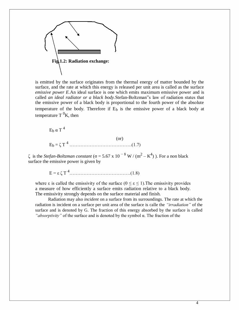
Fig.1.2: Radiation exchange:

is emitted by the surface originates from the thermal energy of matter bounded by the surface, and the rate at which this energy is released per unit area is called as the surface emissive power E.An ideal surface is one which emits maximum emissive power and is called an ideal radiator or a black body.Stefan-Boltzman‟s law of radiation states that the emissive power of a black body is proportional to the fourth power of the absolute

temperature of the body. Therefore if Eb is the emissive power of a black body at

temperature T 0K, then

Eb α T 4

(or)

Eb = ζ T 4 ………………………………….(1.7)

ζ is the Stefan-Boltzman constant (σ = 5.67 x 10 − 8

W / (m2 – K

4) ). For a non black

surface the emissive power is given by

E = ε ζ T 4…………………………………(1.8)

where ε is called the emissivity of the surface (0 ≤ ε ≤ 1).The emissivity provides

a measure of how efficiently a surface emits radiation relative to a black body. The emissivity strongly depends on the surface material and finish.

Radiation may also incident on a surface from its surroundings. The rate at which the

radiation is incident on a surface per unit area of the surface is calle the “irradiation” of the

surface and is denoted by G. The fraction of this energy absorbed by the surface is called

“absorptivity” of the surface and is denoted by the symbol α. The fraction of the

5

incident energy is reflected and is called the “reflectivity” of the surface denoted by ρ and the remaining fraction of the incident energy is transmitted through the surface and

is called the “transmissivity” of the surface denoted by η. It follows from the definitions of α, ρ, and η that

α+ ρ + η = 1 …………………………………….(1.9)

Therefore the energy absorbed by a surface due to any radiation falling on it is given by

Gabs = αG …………………………………(1.10)

The absorptivity α of a body is generally different from its emissivity. However in many practical applications, to simplify the analysis α is assumed to be equal to its

emissivity ε.

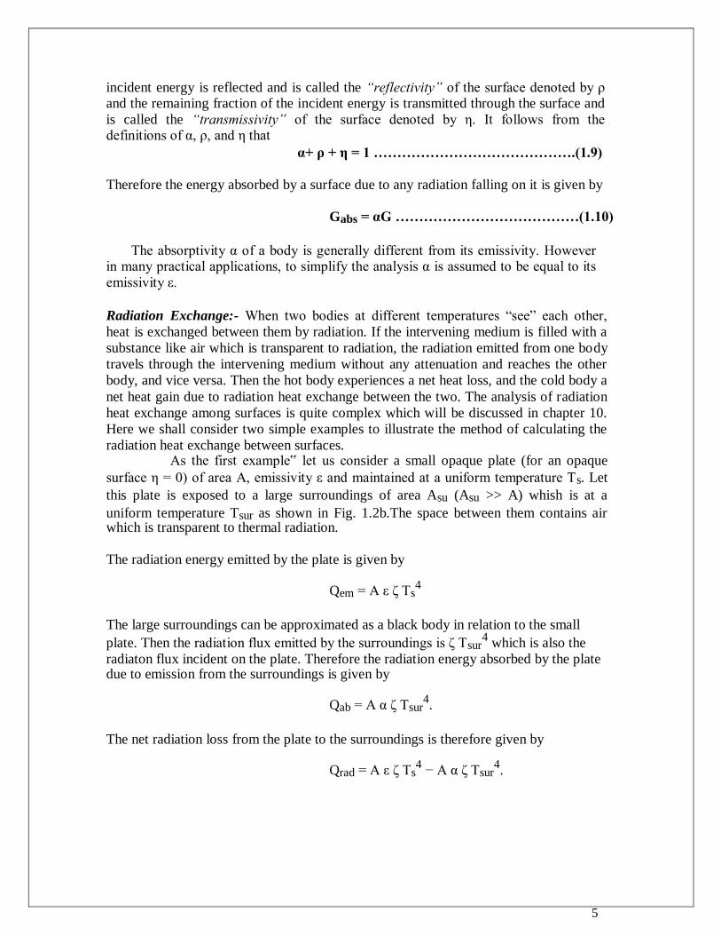
Radiation Exchange:- When two bodies at different temperatures “see” each other,

heat is exchanged between them by radiation. If the intervening medium is filled with a

substance like air which is transparent to radiation, the radiation emitted from one body

travels through the intervening medium without any attenuation and reaches the other

body, and vice versa. Then the hot body experiences a net heat loss, and the cold body a

net heat gain due to radiation heat exchange between the two. The analysis of radiation

heat exchange among surfaces is quite complex which will be discussed in chapter 10.

Here we shall consider two simple examples to illustrate the method of calculating the

radiation heat exchange between surfaces. As the first example‟ let us consider a small opaque plate (for an opaque

surface η = 0) of area A, emissivity ε and maintained at a uniform temperature Ts. Let

this plate is exposed to a large surroundings of area Asu (Asu >> A) whish is at a

uniform temperature Tsur as shown in Fig. 1.2b.The space between them contains air which is transparent to thermal radiation.

The radiation energy emitted by the plate is given by

Qem = A ε ζ Ts4

The large surroundings can be approximated as a black body in relation to the small

plate. Then the radiation flux emitted by the surroundings is ζ Tsur4 which is also the

radiaton flux incident on the plate. Therefore the radiation energy absorbed by the plate due to emission from the surroundings is given by

Qab = A α ζ Tsur4.

The net radiation loss from the plate to the surroundings is therefore given by

Qrad = A ε ζ Ts4 − A α ζ Tsur

4.

6

Assuming α = ε for the plate the above expression for Qnet reduces to

Qrad = A ε ζ [Ts4 – Tsur

4 ] ……………….(1.11)

The above expression can be used to calculate the net radiation heat exchange between a small area and a large surroundings.

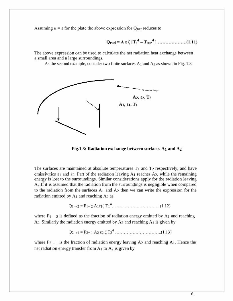
As the second example, consider two finite surfaces A1 and A2 as shown in Fig. 1.3.

Surroundings

A2, ε2, T2

A1, ε1, T1

Fig.1.3: Radiation exchange between surfaces A1 and A2

The surfaces are maintained at absolute temperatures T1 and T2 respectively, and have

emissivities ε1 and ε2. Part of the radiation leaving A1 reaches A2, while the remaining energy is lost to the surroundings. Similar considerations apply for the radiation leaving

A2.If it is assumed that the radiation from the surroundings is negligible when compared

to the radiation from the surfaces A1 and A2 then we can write the expression for the

radiation emitted by A1 and reaching A2 as

Q1→2 = F1− 2 A1ε1ζ T14……………………………(1.12)

where F1 – 2 is defined as the fraction of radiation energy emitted by A1 and reaching

A2. Similarly the radiation energy emitted by A2 and reaching A1 is given by

Q2→1 = F2− 1 A2 ε2 ζ T24 …………………………..(1.13)

where F2 – 1 is the fraction of radiation energy leaving A2 and reaching A1. Hence the

net radiation energy transfer from A1 to A2 is given by

7

Q1 – 2 = Q1→2 − Q2→1

= [F1− 2 A1ε1ζ T14] − [F2− 1 A2 ε2 ζ T2

4]

F1-2 is called the view factor (or geometric shape factor or configuration factor) of A2 with

respect to A1 and F2 - 1 is the view factor of A1 with respect to A2.It will be shown in

chapter 10 that the view factor is purely a geometric property which depends on the relative

orientations of A1 and A2 satisfying the reciprocity relation, A1 F1 – 2 = A2 F2 – 1.

Therefore Q1 – 2 = A1F1 – 2 ζ [ε1 T14 − ε2 T2

4]………………….(1.13)

Radiation Heat Transfer Coefficient:- Under certain restrictive conditions it is possible to simplify the radiation heat transfer calculations by defining a radiation heat transfer

coefficient hr analogous to convective heat transfer coefficient as

Qr = hrA ΔT

For the example of radiation exchange between a surface and the surroundings [Eq. (1. 11)]

using the concept of radiation heat transfer coefficient we can write

Qr = hrA[Ts – Tsur] = A ε ζ [Ts4 – Tsur

4 ]

ε ζ [Ts4 – Tsur

4 ]ε ζ [Ts

2 + Tsur

2 ][Ts + Tsur][Ts – Tsur]

Or hr = --------------------- = -----------------------------------------------

[Ts – Tsur] [Ts – Tsur]

Or hr = ε ζ [Ts2 + Tsur

2 ][Ts + Tsur] ………………………(1.14)

1.3.First Law of Thermodynamics (Law of conservation of energy) as applied to Heat

Transfer Problems :-

The first law of thermodynamics is an essential tool for solving many heat transfer

problems. Hence it is necessary to know the general formulation of the first law of

thermodynamics. First law equation for a control volume:- A control volume is a region in space bounded

by a control surface through which energy and matter may pass.There are two options of

formulating the first law for a control volume. One option is formulating the law on a

rate basis. That is, at any instant, there must be a balance between all energy rates.

Alternatively, the first law must also be satisfied over any time interval Δt. For such an interval, there must be a balance between the amounts of all energy changes.

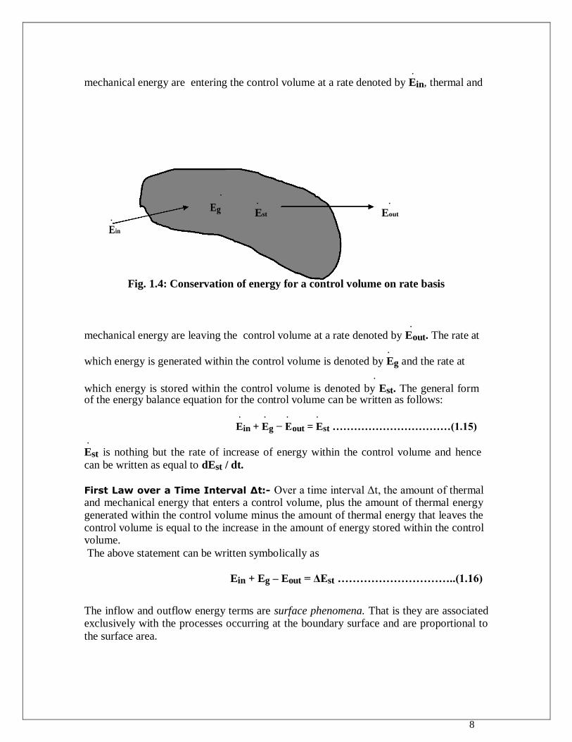
First Law on rate basis: - The rate at which thermal and mechanical energy enters a control volume, plus the rate at which thermal energy is generated within the control volume, minus the rate at which thermal and mechanical energy leaves the control volume must be equal to the rate of increase of stored energy within the control volume. Consider a control volume shown in Fig. 1.4 which shows that thermal and

8

.

mechanical energy are entering the control volume at a rate denoted by Ein, thermal and

.

Eg

. .

Est Eout .

Ein

Fig. 1.4: Conservation of energy for a control volume on rate basis

.

mechanical energy are leaving the control volume at a rate denoted by Eout. The rate at

.

which energy is generated within the control volume is denoted by Eg and the rate at

.

which energy is stored within the control volume is denoted by Est. The general form of the energy balance equation for the control volume can be written as follows:

. . . .

Ein + Eg − Eout = Est ……………………………(1.15)

.

Est is nothing but the rate of increase of energy within the control volume and hence

can be written as equal to dEst / dt.

First Law over a Time Interval Δt:- Over a time interval Δt, the amount of thermal and mechanical energy that enters a control volume, plus the amount of thermal energy generated within the control volume minus the amount of thermal energy that leaves the control volume is equal to the increase in the amount of energy stored within the control volume. The above statement can be written symbolically as

Ein + Eg – Eout = ΔEst …………………………..(1.16)

The inflow and outflow energy terms are surface phenomena. That is they are associated exclusively with the processes occurring at the boundary surface and are proportional to

the surface area.

9

The energy generation term is associated with conversion from some other form

(chemical, electrical, electromagnetic, or nuclear) to thermal energy. It is a volumetric

phenomenon.That is, it occurs within the control volume and is proportional to the magnitude

of this volume. For example, exothermic chemical reaction may be taking place within the

control volume. This reaction converts chemical energy to thermal energy and we say that

energy is generated within the control volume. Conversion of electrical energy to thermal

energy due to resistance heating when electric current is passed through an electrical

conductor is another example of thermal energy generation Energy storage is also a volumetric phenomenon and energy change within

the control volume is due to the changes in kinetic, potential and internal energy of

matter within the control volume.

1.4. Illustrative Examples: A. Conduction

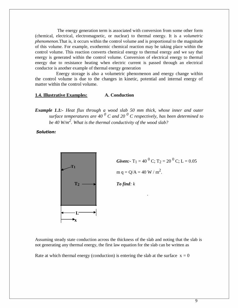
Example 1.1:- Heat flux through a wood slab 50 mm thick, whose inner and outer

surface temperatures are 40 0 C and 20

0 C respectively, has been determined to

be 40 W/m2. What is the thermal conductivity of the wood slab?

Solution:

T1

Given:- T1 = 40 0 C; T2 = 20

0 C; L = 0.05

m q = Q/A = 40 W / m2.

T2 To find: k

.

L

x

Assuming steady state conduction across the thickness of the slab and noting that the slab is

not generating any thermal energy, the first law equation for the slab can be written as

Rate at which thermal energy (conduction) is entering the slab at the surface x = 0

10

is equal to the rate at which thermal energy is leaving the slab at the surface x = L That is

Qx|x = 0 = Qx|x = L = Qx = constant

By Fourier‟s law we have Qx = − kA (dT / dx).

Separating the variables and integrating both sides w.r.t. „x‟ we have

L T2

Qx ∫dx = − kA ∫dT . Or Qx = kA (T1 – T2) / L 0 T1

Heat flux = q = Qx / A = k(T1 – T2) / L

Hence

k = q L / (T1 – T2) = 40 x 0.05 / (40 – 20) = 0.1 W / (m – K)

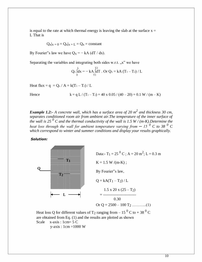
Example 1.2:- A concrete wall, which has a surface area of 20 m2 and thickness 30 cm,

separates conditioned room air from ambient air.The temperature of the inner surface of

the wall is 25 0 C and the thermal conductivity of the wall is 1.5 W / (m-K).Determine the

heat loss through the wall for ambient temperature varying from ─ 15 0 C to 38

0 C

which correspond to winter and summer conditions and display your results graphically.

Solution:

Data:- T1 = 25 0 C ; A = 20 m

2; L = 0.3 m

T1 K = 1.5 W /(m-K) ;

Q By Fourier‟s law,

T2

Q = kA(T1 – T2) / L

1.5 x 20 x (25 – T2)

L = -------------------------

0.30

Or Q = 2500 – 100 T2 ………..(1)

Heat loss Q for different values of T2 ranging from – 15 0 C to + 38

0 C

are obtained from Eq. (1) and the results are plotted as shown

Scale x-axis : 1cm= 5 C y-axis : 1cm =1000 W

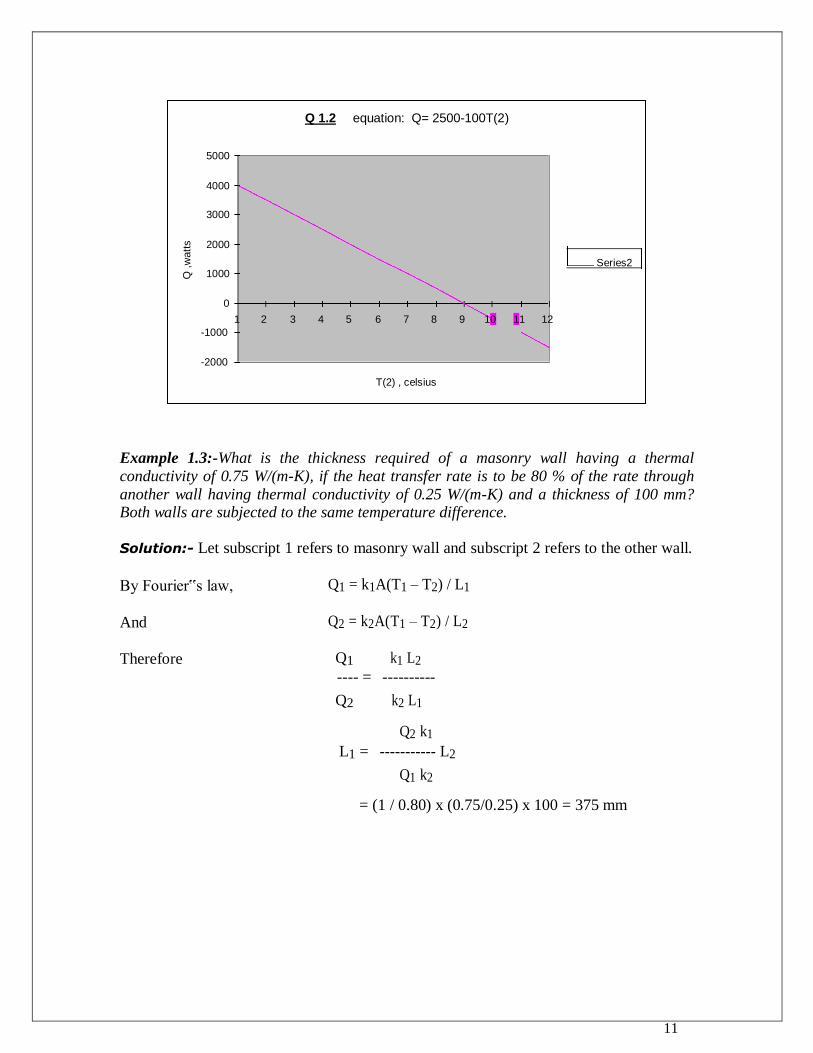
11

Q 1.2 equation: Q= 2500-100T(2)

Q ,w

att

s

5000

4000

3000

2000

1000

Series2

0 1 2 3 4 5 6 7 8 9 10 11 12

-1000

-2000

T(2) , celsius

Example 1.3:-What is the thickness required of a masonry wall having a thermal

conductivity of 0.75 W/(m-K), if the heat transfer rate is to be 80 % of the rate through

another wall having thermal conductivity of 0.25 W/(m-K) and a thickness of 100 mm? Both walls are subjected to the same temperature difference.

Solution:- Let subscript 1 refers to masonry wall and subscript 2 refers to the other wall.

By Fourier‟s law, Q1 = k1A(T1 – T2) / L1

And Q2 = k2A(T1 – T2) / L2

Therefore Q1 k1 L2

---- = ----------

Q2 k2 L1

Q2 k1

L1 = ----------- L2

Q1 k2

= (1 / 0.80) x (0.75/0.25) x 100 = 375 mm

12

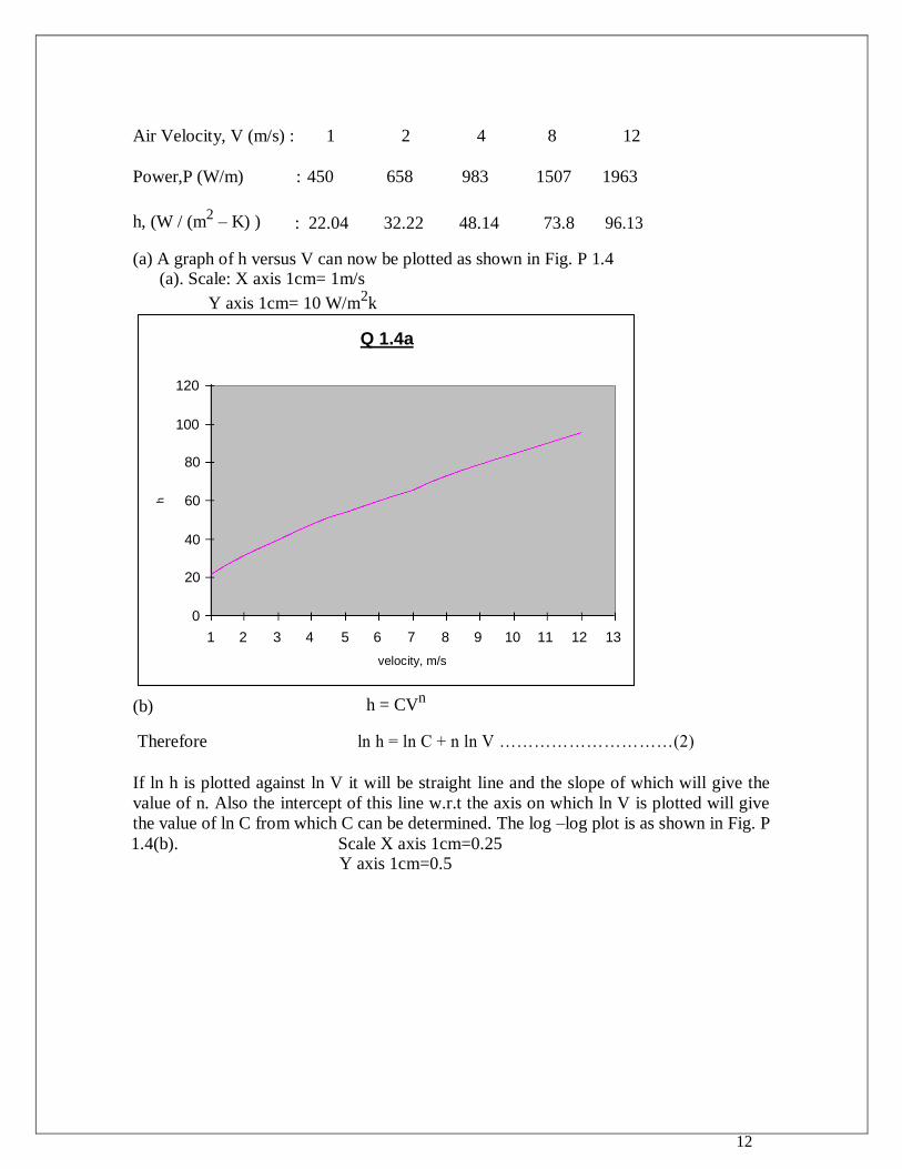
Air Velocity, V (m/s) : 1 2 4 8 12

Power,P (W/m) : 450 658 983 1507 1963

h, (W / (m2 – K) ) : 22.04 32.22 48.14 73.8 96.13

(a) A graph of h versus V can now be plotted as shown in Fig. P 1.4 (a). Scale: X axis 1cm= 1m/s

Y axis 1cm= 10 W/m2k

Q 1.4a

h

120

100

80

60

40

20

0

1 2 3 4 5 6 7 8 9 10 11 12 13

velocity, m/s

(b) h = CVn

Therefore ln h = ln C + n ln V …………………………(2)

If ln h is plotted against ln V it will be straight line and the slope of which will give the

value of n. Also the intercept of this line w.r.t the axis on which ln V is plotted will give

the value of ln C from which C can be determined. The log –log plot is as shown in Fig. P 1.4(b). Scale X axis 1cm=0.25

Y axis 1cm=0.5

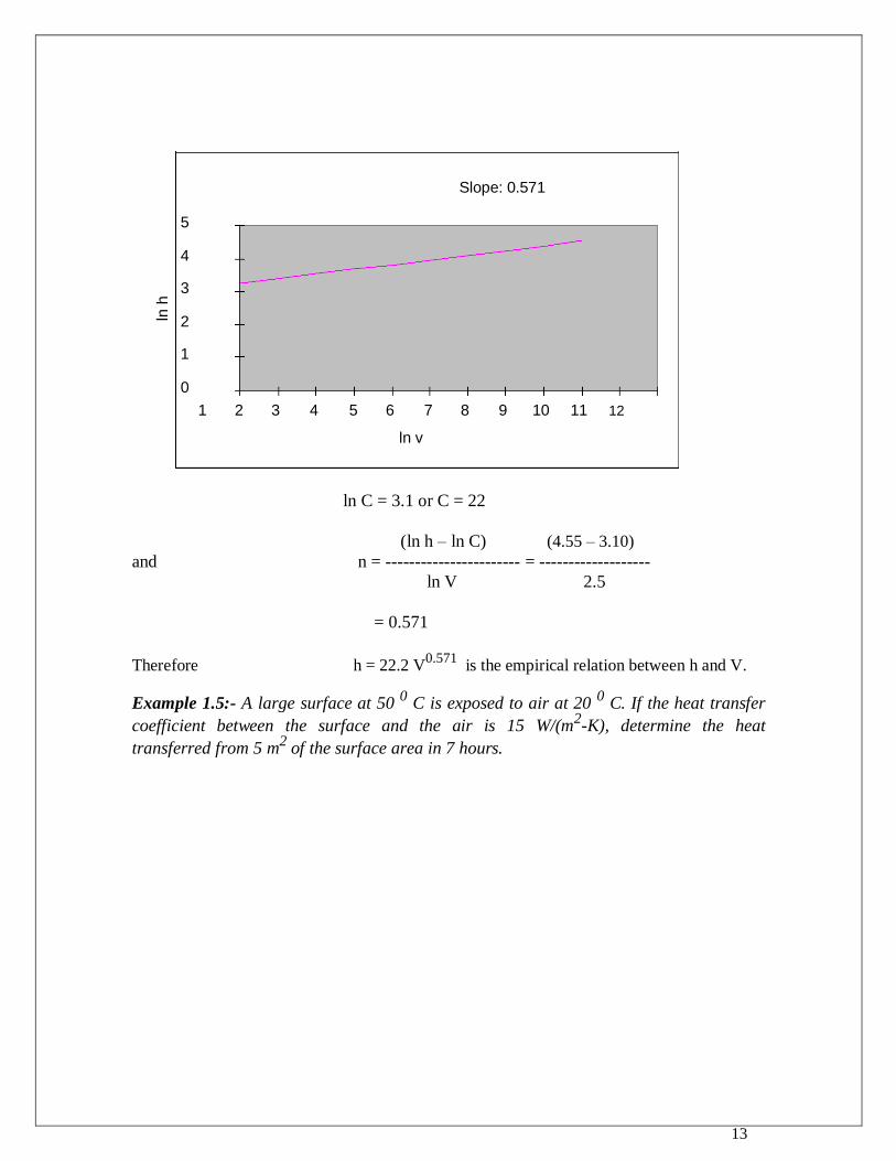
13

ln h

Slope: 0.571

5

4

3

2

1

0

1 2 3 4 5 6 7 8 9 10 11 12

ln v

ln C = 3.1 or C = 22

(ln h – ln C) (4.55 – 3.10) and n = ----------------------- = -------------------

ln V 2.5

= 0.571

Therefore h = 22.2 V0.571

is the empirical relation between h and V.

Example 1.5:- A large surface at 50 0 C is exposed to air at 20

0 C. If the heat transfer

coefficient between the surface and the air is 15 W/(m2-K), determine the heat

transferred from 5 m2 of the surface area in 7 hours.

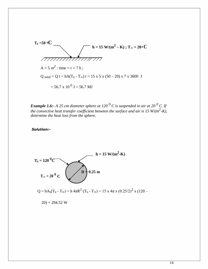
14

Ts =50 0C h = 15 W/(m

2 – K) ; T∞ = 20 0 C

A = 5 m2 : time = t = 7 h ;

Q total = Q t = hA(Ts - T∞) t = 15 x 5 x (50 – 20) x 7 x 3600 J

= 56.7 x 10 6 J = 56.7 MJ

Example 1.6:- A 25 cm diameter sphere at 120 0 C is suspended in air at 20

0 C. If

the convective heat transfer coefficient between the surface and air is 15 W/(m2-K),

determine the heat loss from the sphere.

Solution:-

h = 15 W/(m2-K)

Ts = 120 0C

T∞ = 20 0

C

D = 0.25 m

Q = hAs(Ts - T∞) = h 4πR2 (Ts - T∞) = 15 x 4π x (0.25/2)

2 x (120 –

20) = 294.52 W

15

C. Radiation:

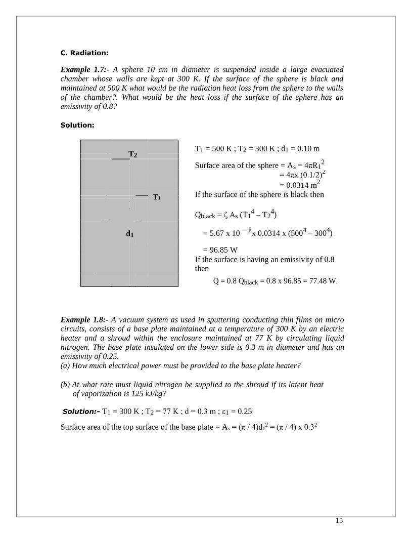
Example 1.7:- A sphere 10 cm in diameter is suspended inside a large evacuated

chamber whose walls are kept at 300 K. If the surface of the sphere is black and

maintained at 500 K what would be the radiation heat loss from the sphere to the walls

of the chamber?. What would be the heat loss if the surface of the sphere has an

emissivity of 0.8?

Solution:

T2

T1 = 500 K ; T2 = 300 K ; d1 = 0.10 m

Surface area of the sphere = As = 4πR12

= 4πx (0.1/2)2

= 0.0314 m2

T1 If the surface of the sphere is black then

Qblack = ζ As (T14 – T2

4)

d1 = 5.67 x 10 ─ 8

x 0.0314 x (5004 – 300

4)

= 96.85 W

If the surface is having an emissivity of 0.8

then

Q = 0.8 Qblack = 0.8 x 96.85 = 77.48 W.

Example 1.8:- A vacuum system as used in sputtering conducting thin films on micro

circuits, consists of a base plate maintained at a temperature of 300 K by an electric

heater and a shroud within the enclosure maintained at 77 K by circulating liquid

nitrogen. The base plate insulated on the lower side is 0.3 m in diameter and has an

emissivity of 0.25. (a) How much electrical power must be provided to the base plate heater?

(b) At what rate must liquid nitrogen be supplied to the shroud if its latent heat

of vaporization is 125 kJ/kg?

Solution:- T1 = 300 K ; T2 = 77 K ; d = 0.3 m ; ε1 = 0.25

Surface area of the top surface of the base plate = As = (π / 4)d12 = (π / 4) x 0.32

16

= 0.0707 m2

(a) Qr = ε1ζ As (T14 – T2

4)

= 0.25 x 5.67 x 10 ─ 8

x 0.0707 x (3004 – 77

4) = 8.08 W

.

(b) If mN2 = mass flow rate of nitrogen that is vapourised then

. 8.08

mN2 = Qr / hfg = ---------------- = 6.464 x 10-5

kg/s or 0.233 kg/s

125 x 1000

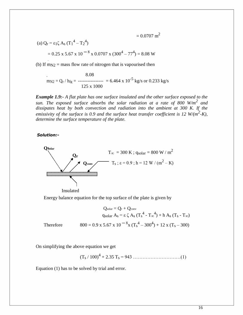
Example 1.9:- A flat plate has one surface insulated and the other surface exposed to the

sun. The exposed surface absorbs the solar radiation at a rate of 800 W/m2 and

dissipates heat by both convection and radiation into the ambient at 300 K. If the

emissivity of the surface is 0.9 and the surface heat transfer coefficient is 12 W/(m2-K),

determine the surface temperature of the plate.

Solution:-

Qsolar T∞ = 300 K ; qsolar = 800 W / m

2

Qr

Qconv

Ts ; ε = 0.9 ; h = 12 W / (m2 – K)

Insulated

Energy balance equation for the top surface of the plate is given by

Qsolar = Qr + Qconv

qsolar As = ε ζ As (Ts4 - T∞

4) + h As (Ts - T∞)

Therefore 800 = 0.9 x 5.67 x 10 ─ 8

x (Ts4 – 300

4) + 12 x (Ts – 300)

On simplifying the above equation we get

(Ts / 100)4 + 2.35 Ts = 943 …………………………(1)

Equation (1) has to be solved by trial and error.

17

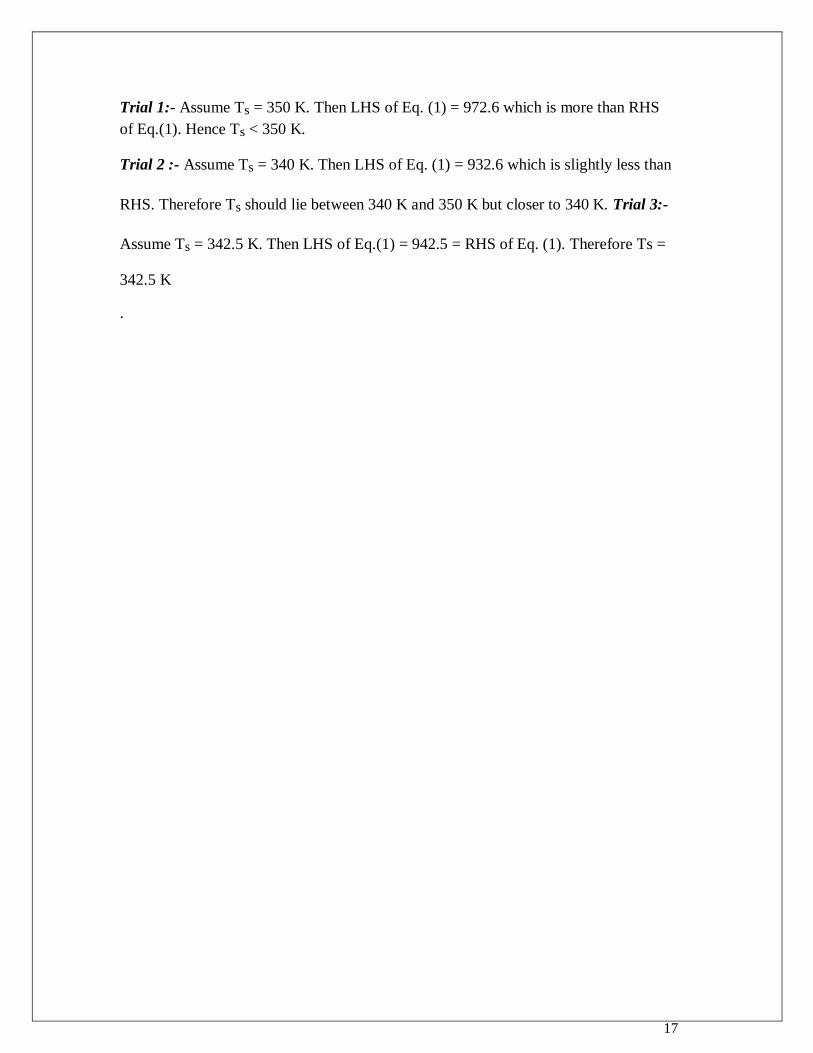
Trial 1:- Assume Ts = 350 K. Then LHS of Eq. (1) = 972.6 which is more than RHS

of Eq.(1). Hence Ts < 350 K.

Trial 2 :- Assume Ts = 340 K. Then LHS of Eq. (1) = 932.6 which is slightly less than

RHS. Therefore Ts should lie between 340 K and 350 K but closer to 340 K. Trial 3:-

Assume Ts = 342.5 K. Then LHS of Eq.(1) = 942.5 = RHS of Eq. (1). Therefore Ts =

342.5 K

.

18

UNIT-II

GOVERNING EQUATIONS OF CONDUCTION

Introduction: In this chapter, the governing basic equations for conduction in

Cartesian coordinate system is derived. The corresponding equations in cylindrical and

spherical coordinate systems are also mentioned. Mathematical representations of

different types of boundary conditions and the initial condition required to solve

conduction problems are also discussed. After studying this chapter, the student will

be able to write down the governing equation and the required boundary conditions

and initial condition if required for any conduction problem.

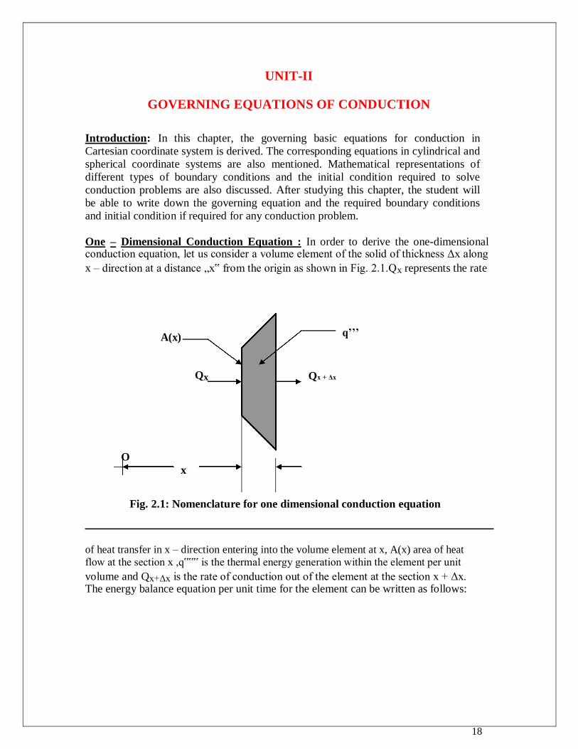
One – Dimensional Conduction Equation : In order to derive the one-dimensional conduction equation, let us consider a volume element of the solid of thickness Δx along

x – direction at a distance „x‟ from the origin as shown in Fig. 2.1.Qx represents the rate

A(x)

q’’’

Qx Qx + Δx

O x

Fig. 2.1: Nomenclature for one dimensional conduction equation

of heat transfer in x – direction entering into the volume element at x, A(x) area of heat

flow at the section x ,q‟‟‟ is the thermal energy generation within the element per unit

volume and Qx+Δx is the rate of conduction out of the element at the section x + Δx. The energy balance equation per unit time for the element can be written as follows:

19

[ Rate of heat conduction into the element at x + Rate of thermal energy generation within the element − Rate of heat conduction out of the element at x + Δx ]

= Rate of increase of internal energy of the element.

i.e.,

Qx + Qg – Qx+Δx = ∂E / ∂t

or Qx + q‟‟‟ A(x) Δx – {Qx + (∂Qx / ∂x)Δx + (∂2Qx / ∂x2)(Δx)2 / 2! + …….}

= ∂/ ∂t (ρA(x)ΔxCpT)

Neglecting higher order terms and noting that ρ and Cp are constants the above equation simplifies to

Qx + q‟‟‟ A(x) Δx – {Qx + (∂Qx / ∂x)Δx = ρA(x)ΔxCp (∂T/ ∂t)

Or

− (∂Qx / ∂x) + q‟‟‟ A(x) = ρA(x) Cp (∂T/ ∂t)

Using Fourier‟s law of conduction , Qx = − k A(x) (∂T / ∂x), the above equation simplifies to

− ∂/ ∂x {− k A(x) (∂T / ∂x)} + q‟‟‟ A(x) = ρA(x) Cp (∂T/ ∂t)

Or {1/A(x)} ∂/ ∂x {k A(x) (∂T / ∂x)} + q’’’ = ρ Cp (∂T/ ∂t) ……………(2.1)

Eq. (2.1) is the most general form of conduction equation for one-dimensional unsteady state conduction.

2.2.1.Equation for one-dimensional conduction in plane walls :- For plane walls, the

area of heat flow A(x) is a constant. Hence Eq. (2.1) reduces to the form

∂/ ∂x {k (∂T / ∂x)} + q’’’ = ρ Cp (∂T/ ∂t) …………………(2.2)

(i) If the thermal conductivity of the solid is constant then the above equation reduces to

(∂2T / ∂x

2) + (q’’’ / k) = (1/α )(∂T/ ∂t) ………………………(2.3)

(ii) For steady state conduction problems in solids of constant thermal conductivity temperature within the solid will be independent of time (i.e.(∂T/ ∂t) = 0) and hence Eq. (2.3) reduces to

(d2T / dx

2 )+ (q’’’ / k) = 0………………………………….(2.4)

20

(iii) For a solid of constant thermal conductivity for which there is no thermal

energy generation within the solid q‟‟‟ = 0 and the governing for steady state conduction is obtained by putting q‟‟‟ = 0 in Eq. (2.4) as

(d2T / dx

2 ) = 0 ………………………………(2.4)

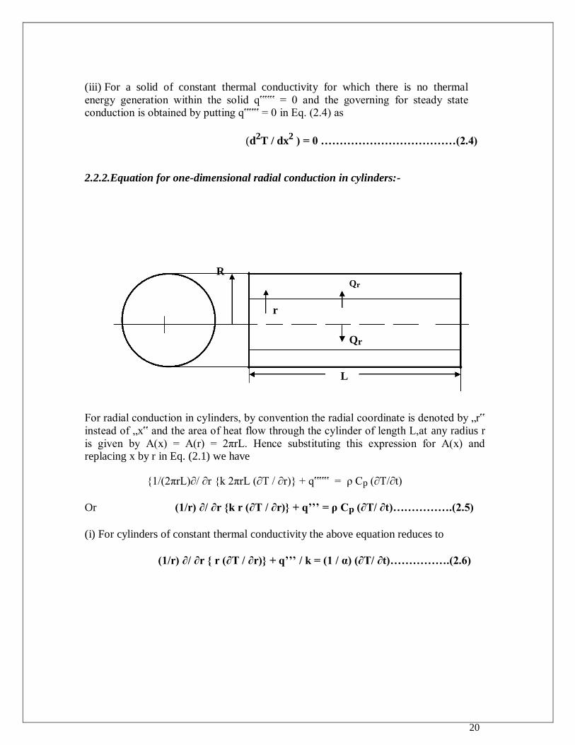
2.2.2.Equation for one-dimensional radial conduction in cylinders:-

R

Qr

r

Qr

L

For radial conduction in cylinders, by convention the radial coordinate is denoted by „r‟

instead of „x‟ and the area of heat flow through the cylinder of length L,at any radius r

is given by A(x) = A(r) = 2πrL. Hence substituting this expression for A(x) and replacing x by r in Eq. (2.1) we have

{1/(2πrL)∂/ ∂r {k 2πrL (∂T / ∂r)} + q‟‟‟ = ρ Cp (∂T/∂t)

Or (1/r) ∂/ ∂r {k r (∂T / ∂r)} + q’’’ = ρ Cp (∂T/ ∂t)…………….(2.5)

(i) For cylinders of constant thermal conductivity the above equation reduces to

(1/r) ∂/ ∂r { r (∂T / ∂r)} + q’’’ / k = (1 / α) (∂T/ ∂t)…………….(2.6)

21

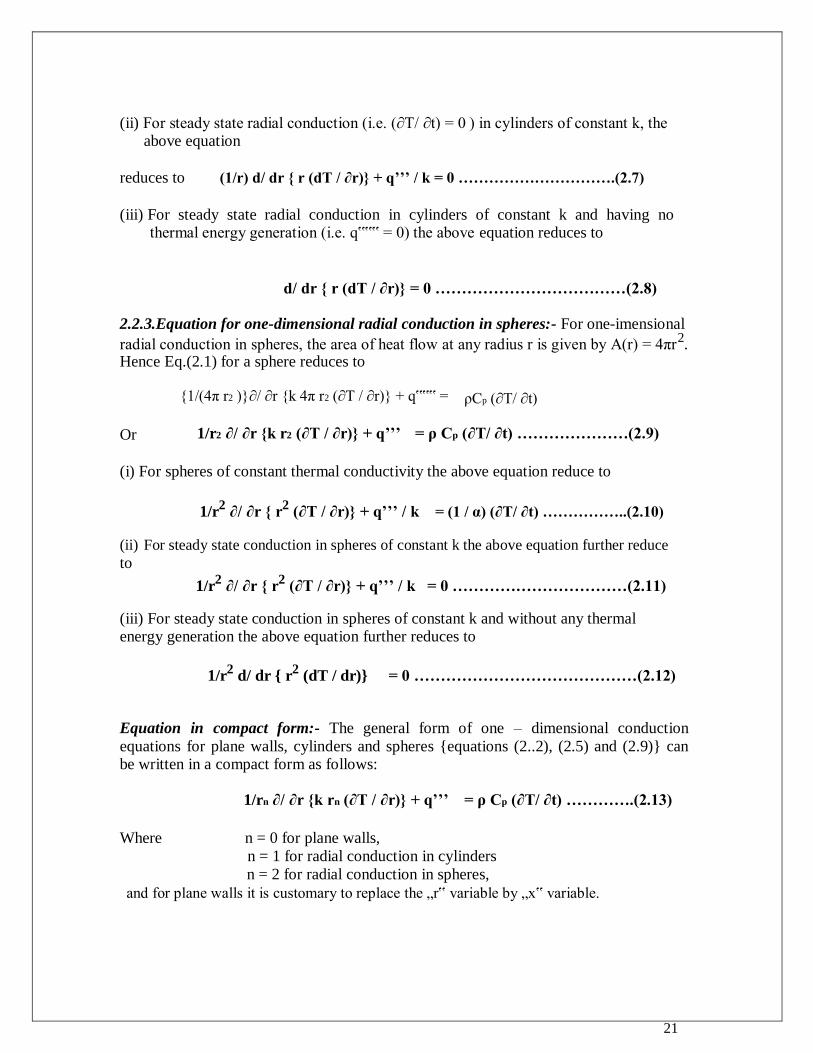
(ii) For steady state radial conduction (i.e. (∂T/ ∂t) = 0 ) in cylinders of constant k, the above equation

reduces to (1/r) d/ dr { r (dT / ∂r)} + q’’’ / k = 0 ………………………….(2.7)

(iii) For steady state radial conduction in cylinders of constant k and having no thermal energy generation (i.e. q‟‟‟ = 0) the above equation reduces to

d/ dr { r (dT / ∂r)} = 0 ………………………………(2.8)

2.2.3.Equation for one-dimensional radial conduction in spheres:- For one-imensional

radial conduction in spheres, the area of heat flow at any radius r is given by A(r) = 4πr2.

Hence Eq.(2.1) for a sphere reduces to

{1/(4π r2 )}∂/ ∂r {k 4π r2 (∂T / ∂r)} + q‟‟‟ =

ρCp (∂T/ ∂t)

Or

1/r2 ∂/ ∂r {k r2 (∂T / ∂r)} + q’’’ = ρ Cp (∂T/ ∂t) …………………(2.9)

(i) For spheres of constant thermal conductivity the above equation reduce to

1/r2 ∂/ ∂r { r

2 (∂T / ∂r)} + q’’’ / k = (1 / α) (∂T/ ∂t) ……………..(2.10)

(ii) For steady state conduction in spheres of constant k the above equation further reduce

to

1/r2 ∂/ ∂r { r

2 (∂T / ∂r)} + q’’’ / k = 0 ……………………………(2.11)

(iii) For steady state conduction in spheres of constant k and without any thermal energy generation the above equation further reduces to

1/r2 d/ dr { r

2 (dT / dr)} = 0 ……………………………………(2.12)

Equation in compact form:- The general form of one – dimensional conduction

equations for plane walls, cylinders and spheres {equations (2..2), (2.5) and (2.9)} can be written in a compact form as follows:

1/rn ∂/ ∂r {k rn (∂T / ∂r)} + q’’’ = ρ Cp (∂T/ ∂t) ………….(2.13)

Where n = 0 for plane walls,

n = 1 for radial conduction in cylinders n = 2 for radial conduction in spheres,

and for plane walls it is customary to replace the „r‟ variable by „x‟ variable.

22

2.3.Three dimensional conduction equations: While deriving the one – dimensional

conduction equation, we assumed that conduction heat transfer is taking place only along

one direction. By allowing conduction along the remaining two directions and following the

same procedure we obtain the governing equation for conduction in three dimenions.

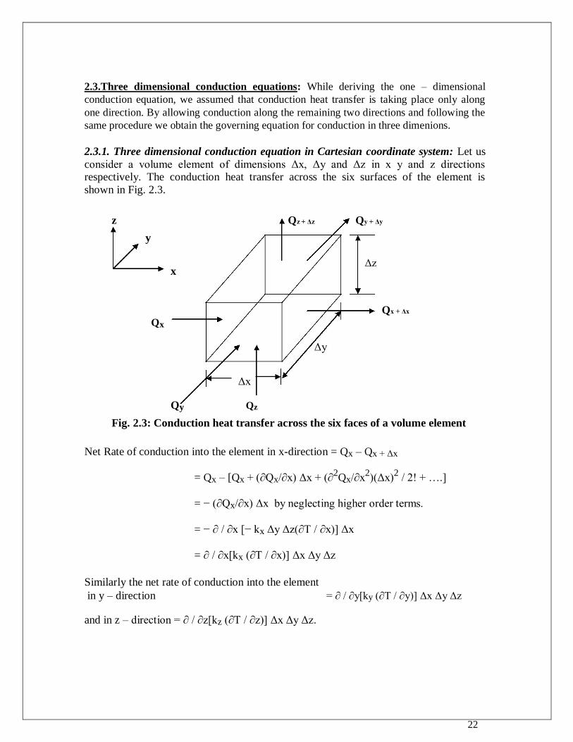
2.3.1. Three dimensional conduction equation in Cartesian coordinate system: Let us

consider a volume element of dimensions Δx, Δy and Δz in x y and z directions respectively. The conduction heat transfer across the six surfaces of the element is

shown in Fig. 2.3.

z Qz + Δz Qy + Δy

y

x

Δz

Qx + Δx

Qx

Δy

Δx

Qy Qz

Fig. 2.3: Conduction heat transfer across the six faces of a volume element

Net Rate of conduction into the element in x-direction = Qx – Qx + Δx

= Qx – [Qx + (∂Qx/∂x) Δx + (∂2Qx/∂x

2)(Δx)

2 / 2! + ….]

= − (∂Qx/∂x) Δx by neglecting higher order terms.

= − ∂ / ∂x [− kx Δy Δz(∂T / ∂x)] Δx

= ∂ / ∂x[kx (∂T / ∂x)] Δx Δy Δz

Similarly the net rate of conduction into the element

in y – direction = ∂ / ∂y[ky (∂T / ∂y)] Δx Δy Δz

and in z – direction = ∂ / ∂z[kz (∂T / ∂z)] Δx Δy Δz.

23

Hence the net rate of conduction into the element from all the three directions

Qin = {∂ / ∂x[kx (∂T / ∂x)] + ∂ / ∂y[ky (∂T / ∂y)] + ∂ / ∂z[kz (∂T / ∂z)] } Δx Δy Δz

Rate of heat thermal energy generation in the element = Qg = q‟‟‟ Δx Δy Δz

Rate of increase of internal energy within the element = ∂E / ∂t = ρ Δx Δy Δz Cp (∂T /

∂t) Applying I law of thermodynamics for the volume element we have

Qin + Qg = ∂E / ∂t

Substituting the expressions for Qin, Qg and ∂E / ∂t and simplifying we get

{∂ / ∂x[kx (∂T / ∂x)] + ∂ / ∂y[ky (∂T / ∂y)] + ∂ / ∂z[kz (∂T / ∂z)] } + q’’’ = ρ Cp (∂T / ∂t)

……………………(2.14)

Equation (2.14) is the most general form of conduction equation in Cartesian coordinate system. This equation reduces to much simpler form for many special cases as

indicated below. Special cases:- (i) For isotropic solids, thermal conductivity is independent of

direction; i.e., kx = ky = k z = k. Hence Eq. (2.14) reduces to

{∂ / ∂x[k (∂T / ∂x)] + ∂ / ∂y[k (∂T / ∂y)] + ∂ / ∂z[k (∂T / ∂z)] } + q’’’ = ρ Cp (∂T / ∂t)

……………………..(2.15) (ii) For isotropic solids with constant thermal conductivity the above equation further reduces to

∂2T / ∂x

2 + ∂

2T / ∂y

2 + ∂

2T / ∂z

2 + q’’’ / k = (1 / α) (∂T / ∂t)…………………….(2.16)

Eq.(2.16) is called as the “Fourier – Biot equation” and it reduces to the following forms under specified conditions as mentioned below:

(iii) Steady state conduction [i.e., (∂T / ∂t) = 0]

∂2T / ∂x

2 + ∂

2T / ∂y

2 + ∂

2T / ∂z

2 + q’’’ / k = 0 …………………………….(2.17)

Eq. (2.17) is called the “Poisson equation”.

(iv) No thermal energy generation [i.e. q‟‟‟ = 0]:

∂2T / ∂x

2 + ∂

2T / ∂y

2 + ∂

2T / ∂z

2 = (1 / α) (∂T / ∂t)……………………………..(2.18)

24

Eq. (2.18) is called the “diffusion equation”.

(v) Steady state conduction without heat generation [i.e., (∂T / ∂t) = 0 and q‟‟‟ = 0]:

∂2T / ∂x

2 + ∂

2T / ∂y

2 + ∂

2T / ∂z

2 = 0 …………………………………………(2.19)

Eq. (2.19) is called the “Laplace equation”.

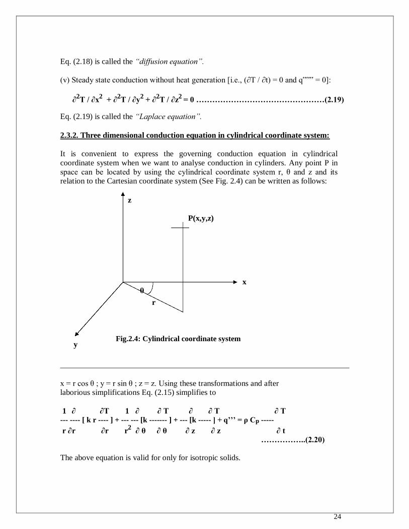
2.3.2. Three dimensional conduction equation in cylindrical coordinate system:

It is convenient to express the governing conduction equation in cylindrical

coordinate system when we want to analyse conduction in cylinders. Any point P in

space can be located by using the cylindrical coordinate system r, θ and z and its relation to the Cartesian coordinate system (See Fig. 2.4) can be written as follows:

y

z

P(x,y,z)

x

θ

r

Fig.2.4: Cylindrical coordinate system

x = r cos θ ; y = r sin θ ; z = z. Using these transformations and after laborious simplifications Eq. (2.15) simplifies to

1 ∂ ∂T 1 ∂ ∂ T ∂ ∂ T ∂ T

--- ---- [ k r ---- ] + --- --- [k ------- ] + --- [k ----- ] + q’’’ = ρ Cp -----

r ∂r ∂r r2 ∂ θ ∂ θ ∂ z ∂ z ∂ t

……………..(2.20)

The above equation is valid for only for isotropic solids.

25

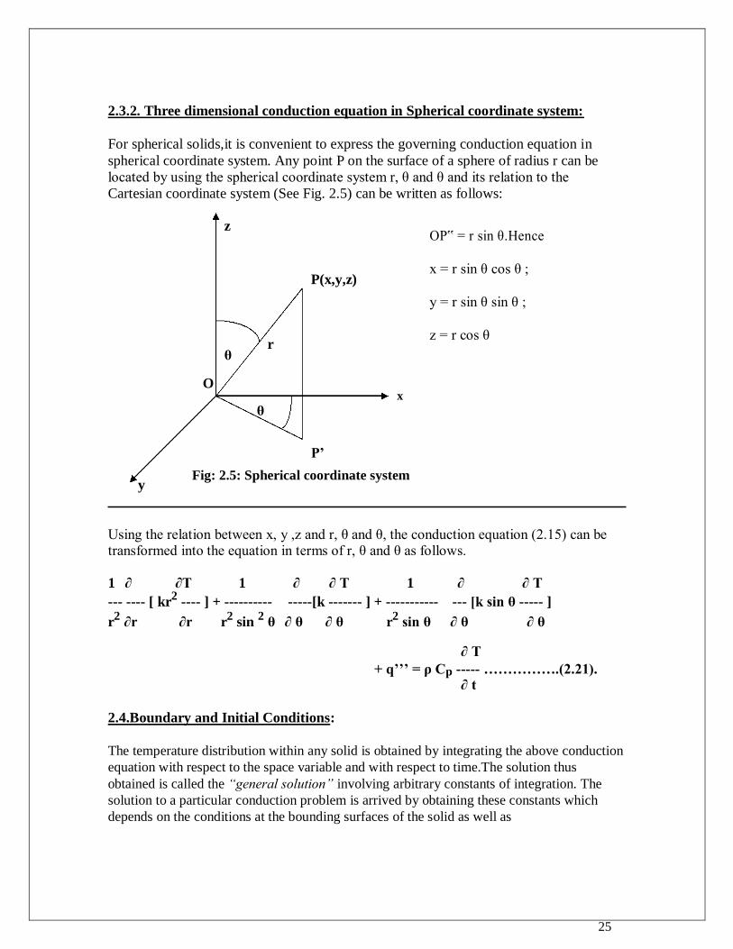
2.3.2. Three dimensional conduction equation in Spherical coordinate system:

For spherical solids,it is convenient to express the governing conduction equation in

spherical coordinate system. Any point P on the surface of a sphere of radius r can be

located by using the spherical coordinate system r, θ and θ and its relation to the

Cartesian coordinate system (See Fig. 2.5) can be written as follows:

z OP‟ = r sin θ.Hence

P(x,y,z)

x = r sin θ cos θ ;

y = r sin θ sin θ ;

r

z = r cos θ

θ

O x

y

θ

P’

Fig: 2.5: Spherical coordinate system

Using the relation between x, y ,z and r, θ and θ, the conduction equation (2.15) can be transformed into the equation in terms of r, θ and θ as follows.

1 ∂ ∂T 1 ∂ ∂ T 1 ∂ ∂ T

--- ---- [ kr2 ---- ] + ---------- -----[k ------- ] + ----------- --- [k sin θ ----- ]

r2 ∂r ∂r r

2 sin

2 θ ∂ θ ∂ θ r

2 sin θ ∂ θ ∂ θ

∂ T

+ q’’’ = ρ Cp ----- …………….(2.21). ∂ t

2.4.Boundary and Initial Conditions:

The temperature distribution within any solid is obtained by integrating the above conduction

equation with respect to the space variable and with respect to time.The solution thus

obtained is called the “general solution” involving arbitrary constants of integration. The

solution to a particular conduction problem is arrived by obtaining these constants which

depends on the conditions at the bounding surfaces of the solid as well as

26

the initial condition. The thermal conditions at the boundary surfaces are called the “boundary conditions” . Boundary conditions normally encountered in practice are:

(i) Specified temperature (also called as boundary condition of the first kind), (ii) Specified heat flux (also known as boundary condition of the second kind), (iii) Convective boundary condition (also known as boundary condition of the third kind) and (iv) radiation boundary condition. The mathematical representations of these boundary

conditions are illustrated by means of a few examples below.

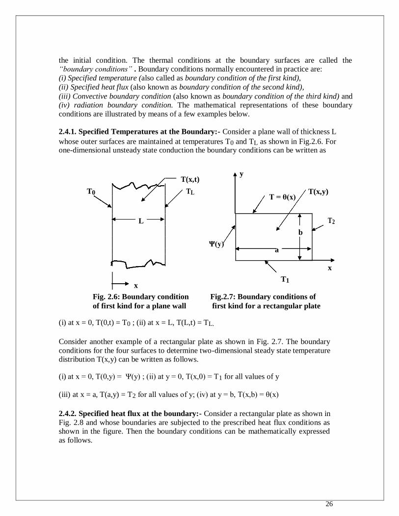
2.4.1. Specified Temperatures at the Boundary:- Consider a plane wall of thickness L

whose outer surfaces are maintained at temperatures T0 and TL as shown in Fig.2.6. For one-dimensional unsteady state conduction the boundary conditions can be written as

T(x,t)

y

T0 TL T = θ(x)

T(x,y)

L

T2

b

Ψ(y) a

x

T1

x

Fig. 2.6: Boundary condition Fig.2.7: Boundary conditions of

of first kind for a plane wall first kind for a rectangular plate

(i) at x = 0, T(0,t) = T0 ; (ii) at x = L, T(L,t) = TL.

Consider another example of a rectangular plate as shown in Fig. 2.7. The boundary

conditions for the four surfaces to determine two-dimensional steady state temperature distribution T(x,y) can be written as follows.

(i) at x = 0, T(0,y) = Ψ(y) ; (ii) at y = 0, T(x,0) = T1 for all values of y

(iii) at x = a, T(a,y) = T2 for all values of y; (iv) at y = b, T(x,b) = θ(x)

2.4.2. Specified heat flux at the boundary:- Consider a rectangular plate as shown in

Fig. 2.8 and whose boundaries are subjected to the prescribed heat flux conditions as shown in the figure. Then the boundary conditions can be mathematically expressed

as follows.

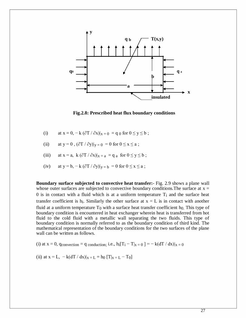
27

y

q b T(x,y)

q0 q a

b

a x

insulated

Fig.2.8: Prescribed heat flux boundary conditions

(i) at x = 0, − k (∂T / ∂x)|x = 0 = q 0 for 0 ≤ y ≤ b ;

(ii) at y = 0 , (∂T / ∂y)|y = 0 = 0 for 0 ≤ x ≤ a ;

(iii) at x = a, k (∂T / ∂x)|x = a = q a for 0 ≤ y ≤ b ;

(iv) at y = b, − k (∂T / ∂y)|y = b = 0 for 0 ≤ x ≤ a ;

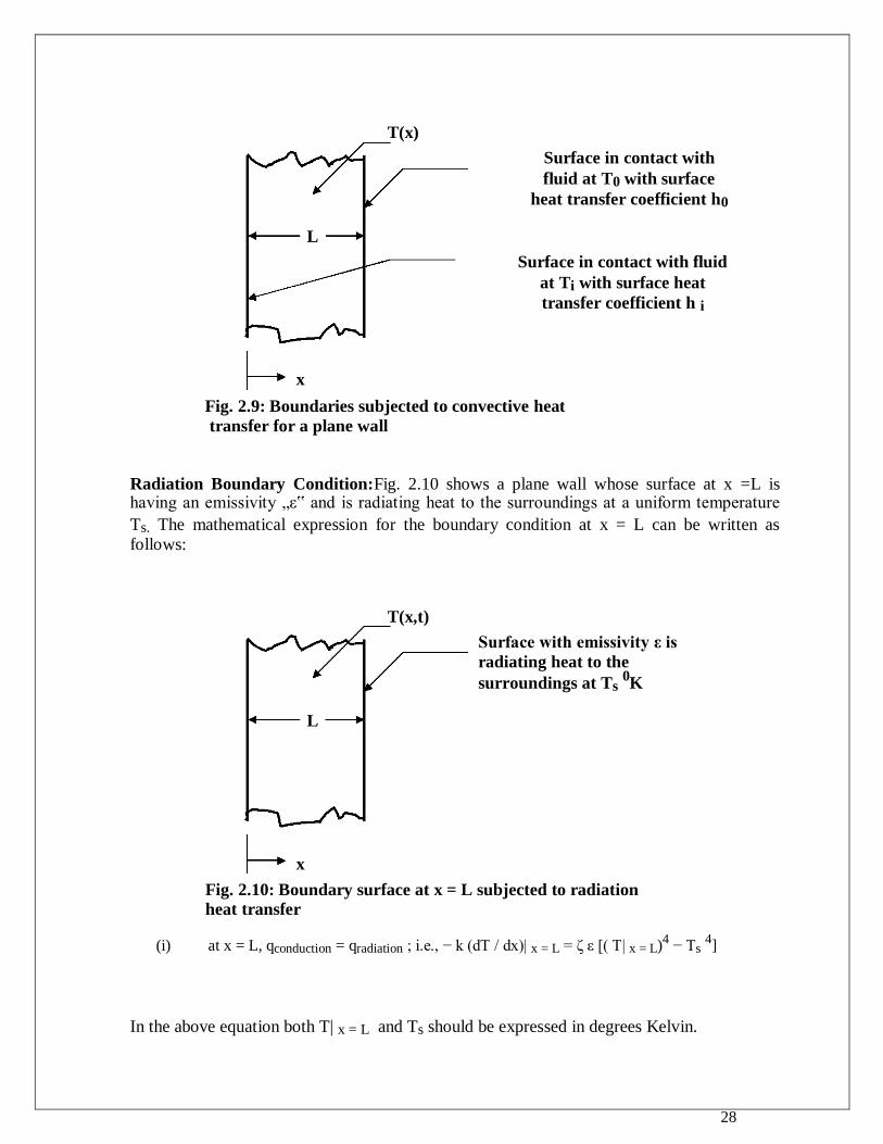
Boundary surface subjected to convective heat transfer:- Fig. 2.9 shows a plane wall whose outer surfaces are subjected to convective boundary conditions.The surface at x =

0 is in contact with a fluid which is at a uniform temperature Ti and the surface heat

transfer coefficient is hi. Similarly the other surface at x = L is in contact with another

fluid at a uniform temperature T0 with a surface heat transfer coefficient h0. This type of boundary condition is encountered in heat exchanger wherein heat is transferred from hot fluid to the cold fluid with a metallic wall separating the two fluids. This type of boundary condition is normally referred to as the boundary condition of third kind. The mathematical representation of the boundary conditions for the two surfaces of the plane wall can be written as follows.

(i) at x = 0, qconvection = q conduction; i.e., hi[Ti − T|x = 0 ] = − k(dT / dx)|x = 0

(ii) at x = L, − k(dT / dx)|x = L = h0 [T|x = L − T0]

28

T(x)

Surface in contact with

fluid at T0 with surface

heat transfer coefficient h0

L

Surface in contact with fluid

at Ti with surface heat

transfer coefficient h i

x

Fig. 2.9: Boundaries subjected to convective heat

transfer for a plane wall

Radiation Boundary Condition:Fig. 2.10 shows a plane wall whose surface at x =L is having an emissivity „ε‟ and is radiating heat to the surroundings at a uniform temperature

Ts. The mathematical expression for the boundary condition at x = L can be written as

follows:

T(x,t)

Surface with emissivity ε is

radiating heat to the

surroundings at Ts 0K

L

x

Fig. 2.10: Boundary surface at x = L subjected to radiation

heat transfer

(i) at x = L, qconduction = qradiation ; i.e., − k (dT / dx)| x = L = ζ ε [( T| x = L)4 − Ts

4]

In the above equation both T| x = L and Ts should be expressed in degrees Kelvin.

29

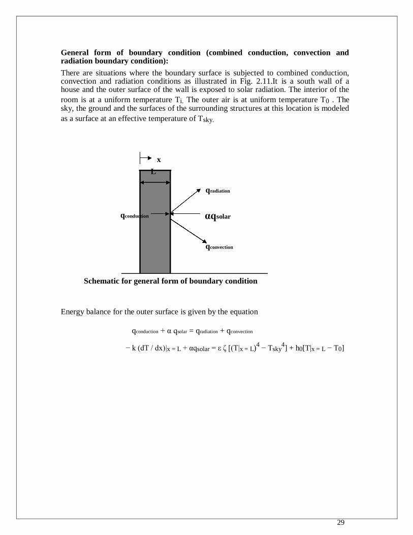
General form of boundary condition (combined conduction, convection and radiation boundary condition):

There are situations where the boundary surface is subjected to combined conduction, convection and radiation conditions as illustrated in Fig. 2.11.It is a south wall of a house and the outer surface of the wall is exposed to solar radiation. The interior of the

room is at a uniform temperature Ti. The outer air is at uniform temperature T0 . The sky, the ground and the surfaces of the surrounding structures at this location is modeled

as a surface at an effective temperature of Tsky.

x

L

qradiation

qconduction αqsolar

qconvection

Schematic for general form of boundary condition

Energy balance for the outer surface is given by the equation

qconduction + α qsolar = qradiation + qconvection

− k (dT / dx)|x = L + αqsolar = ε ζ [(T|x = L)4 − Tsky

4] + h0[T|x = L − T0]

30

B. Mathematical Formulation of Boundary conditions:

A plane wall of thickness L is subjected to a heat supply at a rate of q0 W/m2 at one boundary surface and dissipates heat from the surface by convection to the ambient

which is at a uniform temperature of T∞ with a surface heat transfer coefficient of h∞. Write the mathematical formulation of the boundary conditions for the plane wall.

Consider a solid cylinder of radius R and height Z. The outer curved surface of the

cylinder is subjected to a uniform heating electrically at a rate of q0 W / m2.Both the circular surfaces of the cylinder are exposed to an environment at a uniform temperature T∞ with a surface heat transfer coefficient h. Write the mathematical formulation of the boundary conditions for the solid cylinder.

A hollow cylinder of inner radius ri, outer radius r0 and height H is subjected to the

following boundary conditions. (a) The inner curved surface is heated uniformly with an electric heater at a

constant rate of q0 W/m2, (b) the outer curved surface dissipates heat by convection into an ambient at a

uniform temperature, T∞ with a convective heat transfer coefficient, h (c) the lower flat surface of the cylinder is insulated, and (d) the upper flat surface of the cylinder dissipates heat by convection into the

ambient at T∞ with surface heat transfer coefficient h. Write the mathematical formulation of the boundary conditions for the hollow cylinder.

C. Formulation of Heat Conduction Problems:

A plane wall of thickness L and with constant thermal properties is initially at a uniform temperature Ti. Suddenly one of the surfaces of the wall is subjected to heating by the flow of a hot gas at temperature T∞ and the other surface is kept insulated. The heat transfer coefficient between the hot gas and the surface exposed to it is h. There is no heat generation in the wall. Write the mathematical formulation of the problem to determine the one-dimensional unsteady state temperature within the wall.

A copper bar of radius R is initially at a uniform temperature Ti. Suddenly the heating

of the rod begins at time t=0 by the passage of electric current, which generates heat at a uniform rate of q’’’ W/m2. The outer surface of the dissipates heat into an ambient at a uniform temperature T∞ with a convective heat transfer coefficient h. Assuming that thermal conductivity of the bar to be constant, write the mathematical formulation of the heat conduction problem to determine the one-dimensional radial unsteady state temperature distribution in the rod.

Consider a solid cylinder of radius R and height H. Heat is generated in the solid at a

uniform rate of q’’’ W/m3. One of the circular faces of the cylinder is insulated and the other circular face dissipates heat by convection into a medium at a uniform temperature of T∞ with a surface heat transfer coefficient of h. The outer curved surface of the cylinder is maintained at a uniform temperature of T0. Write the mathematical formulation to determine the two-dimensional steady state temperature distribution T(r, z) in the cylinder.

Consider a rectangular plate as shown in Fig. P2.10.The plate is generating heat at a uniform rate of

q’’’

W/m3. Write the mathematical formulation to determine two-dimensional steady state temperature

distribution in the plate.

31

Consider the north wall of a house of thickness L. The outer surface of the wall exchanges heat by both convection and radiation. The interior of the house is maintained at a uniform temperature of Ti, while the exterior of the house is at a uniform temperature T0. The sky, the ground, and the surfaces of the surrounding structures at this location can be modeled as a surface at an effective temperature of Tsky for radiation heat exchange on the outer surface. The radiation heat exchange between the inner surface of the wall and the surfaces of the other walls, floor and ceiling are negligible. The convective heat transfer coefficient for the inner and outer surfaces of the wall under consideration are hi and h0 respectively. The thermal conductivity of the wall material is K and the emissivity of the outer surface of the wall is ‘ε0’. Assuming the heat transfer through the wall is steady and one dimensional, express the mathematical formulation (differential equation and boundary conditions) of the heat conduction problem

32

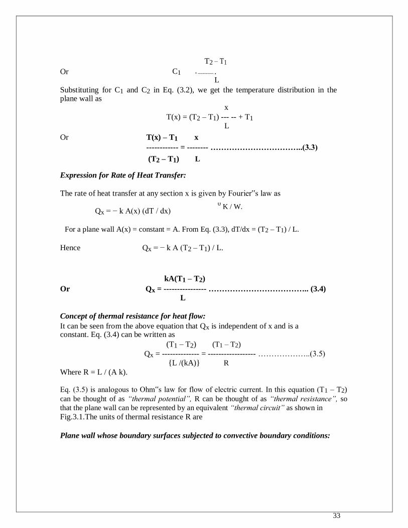
ONE DIMENSIONAL STEADY STATE

CONDUCTION

Conduction Without Heat Generation

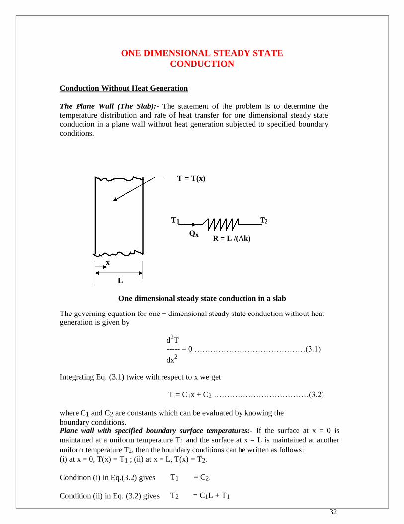
The Plane Wall (The Slab):- The statement of the problem is to determine the

temperature distribution and rate of heat transfer for one dimensional steady state conduction in a plane wall without heat generation subjected to specified boundary

conditions.

T = T(x)

T1 T2

Qx R = L /(Ak)

x

L

One dimensional steady state conduction in a slab

The governing equation for one − dimensional steady state conduction without heat generation is given by

d2T

----- = 0 ……………………………………(3.1)

dx2

Integrating Eq. (3.1) twice with respect to x we get

T = C1x + C2 ………………………………(3.2)

where C1 and C2 are constants which can be evaluated by knowing the

boundary conditions. Plane wall with specified boundary surface temperatures:- If the surface at x = 0 is

maintained at a uniform temperature T1 and the surface at x = L is maintained at another

uniform temperature T2, then the boundary conditions can be written as follows:

(i) at x = 0, T(x) = T1 ; (ii) at x = L, T(x) = T2.

Condition (i) in Eq.(3.2) gives T1 = C2.

Condition (ii) in Eq. (3.2) gives T2 = C1L + T1

33

T2 – T1

Or C1 = ------------- . L

Substituting for C1 and C2 in Eq. (3.2), we get the temperature distribution in the plane wall as

x

T(x) = (T2 – T1) --- -- + T1

L

Or T(x) – T1 x ------------ = -------- ……………………………..(3.3)

(T2 – T1) L

Expression for Rate of Heat Transfer:

The rate of heat transfer at any section x is given by Fourier‟s law as

Qx = − k A(x) (dT / dx)

For a plane wall A(x) = constant = A. From Eq. (3.3), dT/dx = (T2 – T1) / L.

Hence Qx = − k A (T2 – T1) / L.

kA(T1 – T2)

Or Qx = ---------------- ……………………………….. (3.4)

L

Concept of thermal resistance for heat flow:

It can be seen from the above equation that Qx is independent of x and is a constant. Eq. (3.4) can be written as

(T1 – T2) (T1 – T2)

Qx = -------------- = ------------------ ………………..(3.5)

{L /(kA)} R

Where R = L / (A k).

Eq. (3.5) is analogous to Ohm‟s law for flow of electric current. In this equation (T1 – T2)

can be thought of as “thermal potential”, R can be thought of as “thermal resistance”, so

that the plane wall can be represented by an equivalent “thermal circuit” as shown in

Fig.3.1.The units of thermal resistance R are

Plane wall whose boundary surfaces subjected to convective boundary conditions:

0 K / W.

34

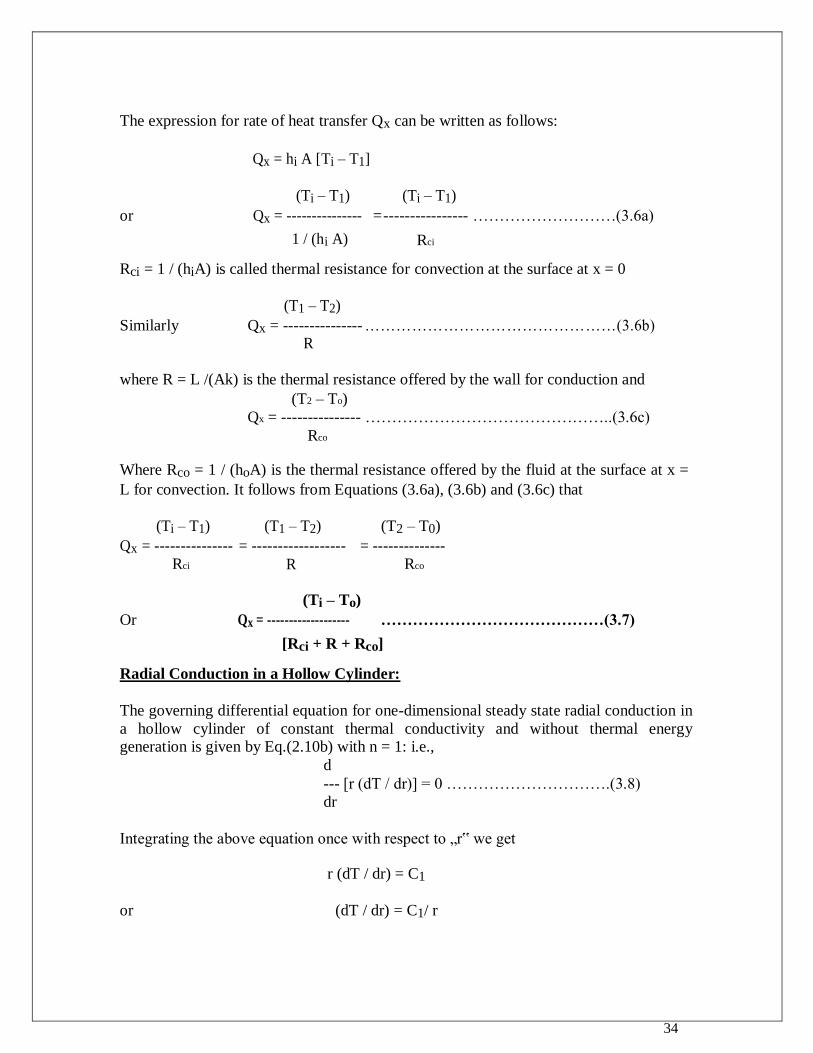
The expression for rate of heat transfer Qx can be written as follows:

Qx = hi A [Ti – T1]

(Ti – T1) (Ti – T1)

or Qx = --------------- = ---------------- ………………………(3.6a)

1 / (hi A) Rci

Rci = 1 / (hiA) is called thermal resistance for convection at the surface at x = 0

(T1 – T2)

Similarly Qx = --------------- …………………………………………(3.6b)

R

where R = L /(Ak) is the thermal resistance offered by the wall for conduction and (T2 – To)

Qx = --------------- ………………………………………..(3.6c) Rco

Where Rco = 1 / (hoA) is the thermal resistance offered by the fluid at the surface at x =

L for convection. It follows from Equations (3.6a), (3.6b) and (3.6c) that

(Ti – T1) (T1 – T2) (T2 – T0)

Qx = --------------- = ------------------ = --------------

Rci R Rco

(Ti – To)

Or Qx = ------------------- ……………………………………(3.7)

[Rci + R + Rco]

Radial Conduction in a Hollow Cylinder:

The governing differential equation for one-dimensional steady state radial conduction in

a hollow cylinder of constant thermal conductivity and without thermal energy generation is given by Eq.(2.10b) with n = 1: i.e.,

d

--- [r (dT / dr)] = 0 ………………………….(3.8) dr

Integrating the above equation once with respect to „r‟ we get

r (dT / dr) = C1

or (dT / dr) = C1/ r

35

Integrating once again with respect to „r‟ we get

T(r) = C1 ln r + C2 ………………………..(3.9)

where C1 and C2 are constants of integration which can be determined by knowing

the boundary conditions of the problem.

Hollow cylinder with prescribed surface temperatures: Let the inner surface at r = r1

be maintained at a uniform temperature T1 and the outer surface at r = r2 be maintained

at another uniform temperature T2 as shown in Fig. 3.3.

Substituting the condition at r1 in Eq.(3.9) we get

T1 = C1 ln r1 + C2 ………………………….(3.10a)

and the condition at r2 in Eq. (3.9) we get

T2 = C1 ln r2 + C2 ………………………….(3.10b)

Solving for C1 and C2 from the above two equations we get

(T1 – T2) (T1 – T2)

C1 = ---------------- = -------------------

[ln r1 – ln r2] ln (r1 / r2)

(T1 – T2)

and C2 = T1 − ------------------ ln r1

ln (r1 / r2)

Substituting these expressions for C1 and C2 in Eq. (3.9) we have

(T1 – T2) (T1 – T2)

T(r) = -------------- ln r + T1 − ---------------- ln r1

ln (r1 / r2) ln (r1 / r2)

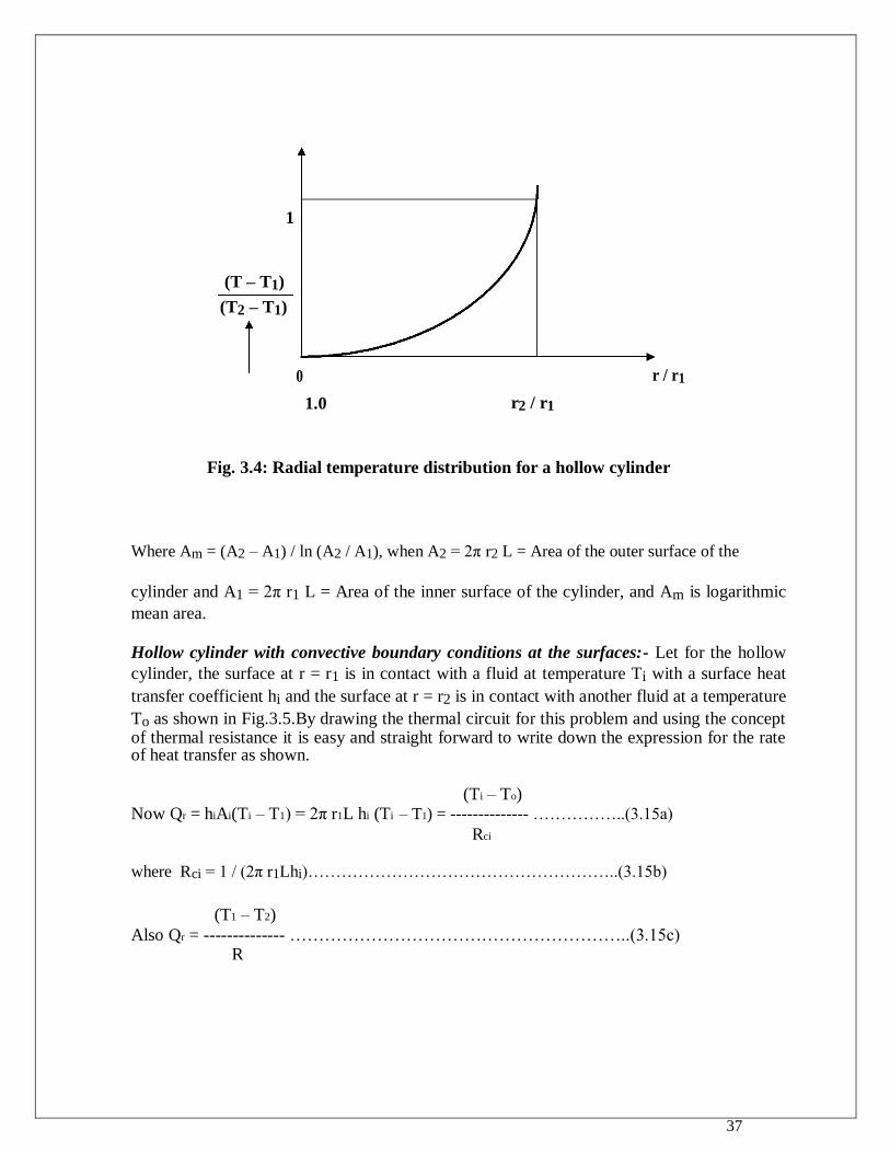
or [T(r) – T1] ln (r / r1) --------------- = ------------------- …………………………………………(3.11)

[ T2 – T1] ln (r2 / r1)

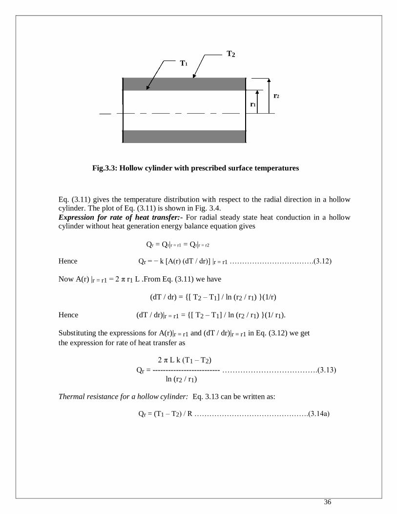
36

T2 T1

r2

r1

Fig.3.3: Hollow cylinder with prescribed surface temperatures

Eq. (3.11) gives the temperature distribution with respect to the radial direction in a hollow cylinder. The plot of Eq. (3.11) is shown in Fig. 3.4. Expression for rate of heat transfer:- For radial steady state heat conduction in a hollow

cylinder without heat generation energy balance equation gives

Qr = Qr|r = r1 = Qr|r = r2

Hence Qr = − k [A(r) (dT / dr)] |r = r1 …………………………….(3.12)

Now A(r) |r = r1 = 2 π r1 L .From Eq. (3.11) we have

(dT / dr) = {[ T2 – T1] / ln (r2 / r1) }(1/r)

Hence (dT / dr)|r = r1 = {[ T2 – T1] / ln (r2 / r1) }(1/ r1).

Substituting the expressions for A(r)|r = r1 and (dT / dr)|r = r1 in Eq. (3.12) we get

the expression for rate of heat transfer as

2 π L k (T1 – T2)

Qr = -------------------------- ……………………………….(3.13)

ln (r2 / r1)

Thermal resistance for a hollow cylinder: Eq. 3.13 can be written as:

Qr = (T1 – T2) / R ……………………………………….(3.14a)

37

1

(T – T1)

(T2 – T1)

0 r / r1

1.0 r2 / r1

Fig. 3.4: Radial temperature distribution for a hollow cylinder

Where Am = (A2 – A1) / ln (A2 / A1), when A2 = 2π r2 L = Area of the outer surface of the

cylinder and A1 = 2π r1 L = Area of the inner surface of the cylinder, and Am is logarithmic

mean area.

Hollow cylinder with convective boundary conditions at the surfaces:- Let for the hollow

cylinder, the surface at r = r1 is in contact with a fluid at temperature Ti with a surface heat

transfer coefficient hi and the surface at r = r2 is in contact with another fluid at a temperature

To as shown in Fig.3.5.By drawing the thermal circuit for this problem and using the concept of thermal resistance it is easy and straight forward to write down the expression for the rate of heat transfer as shown.

Now Qr = hiAi(Ti – T1) = 2π r1L hi (Ti

(Ti – To)

– T1) = -------------- ……………..(3.15a) Rci

where Rci = 1 / (2π r1Lhi)………………………………………………..(3.15b)

(T1 – T2) Also Qr = -------------- …………………………………………………..(3.15c)

R

38

where R = ln (r2 / r1) / (2πLk)…………………………….(3.15d)

Rci + R + Rco

where Rci, R and Rco are given by Eqs.(3.15b), (3.15d) and (3.15f) respectively.

d

--- [r2 (dT / dr)] = 0 ………………………….(3.17)

dr

Integrating the above equation once with respect to „r‟ we get

r2 (dT / dr) = C1

or (dT / dr) = C1/ r2

Integrating once again with respect to „r‟ we get

T(r) = − C1 / r + C2 ………………………..(3.18)

where C1 and C2 are constants of integration which can be determined by knowing

the boundary conditions of the problem.

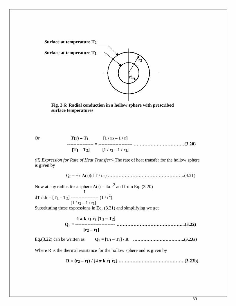
Hollow sphere with prescribed surface temperatures:

(i) Expression for temperature distribution:-Let the inner surface at r = r1 be maintained at a

uniform temperature T1 and the outer surface at r = r2 be maintained at another uniform

temperature T2 as shown in Fig. 3.6.

The boundary conditions for this problem can be written as follows:

(i) at r = r1, T(r) = T1 and (ii) at r = r2, T(r) = T2.

Condition (i) in Eq. (3.18) gives

T1 = − C1 / r1 + C2 ………………………….(3.19a)

Condition (ii) in Eq. (3.18) gives

T2 = − C1

/ r2 + C2 ………………………….(3.19b)

Solving for C1 and C2 from Eqs. (3.19a) and (3.19b) we have

(T1 – T2)

(T1 – T2) C1 = ------------------- and C2 = T1

[1 / r2 – 1 / r1]

+ --------------------------

r1[1 / r2 – 1 / r1]

Substituting these expressions for C1 and C2

in Eq. (3.18) we get

T(r) =

(T1 – T2) / r (T1 – T2) / r1

− ----------------------- + T1 + ---------------------- [1 / r2 – 1 / r1] [1 / r2 – 1 / r1]

39

Surface at temperature T2

Surface at temperature T1

r2

r1

Fig. 3.6: Radial conduction in a hollow sphere with prescribed

surface temperatures

Or T(r) – T1 [1 / r2 – 1 / r] ----------------- = ---------------------- ……………………………(3.20)

[T1 – T2] [1 / r2 – 1 / r1]

(ii) Expression for Rate of Heat Transfer:- The rate of heat transfer for the hollow sphere

is given by

Qr = −k A(r)(d T / dr) …………………………………………..(3.21)

Now at any radius for a sphere A(r) = 4π r2 and from Eq. (3.20)

1

dT / dr = [T1 – T2] ------------------ (1 / r2)

[1 / r2 – 1 / r1]

Substituting these expressions in Eq. (3.21) and simplifying we get

4 π k r1 r2 [T1 – T2]

Qr = -------------------------- ……………………………………...(3.22)

[r2 – r1]

Eq.(3.22) can be written as Qr = [T1 – T2] / R ……………………………..(3.23a)

Where R is the thermal resistance for the hollow sphere and is given by

R = (r2 – r1) / {4 π k r1 r2} …………………………………….(3.23b)

40

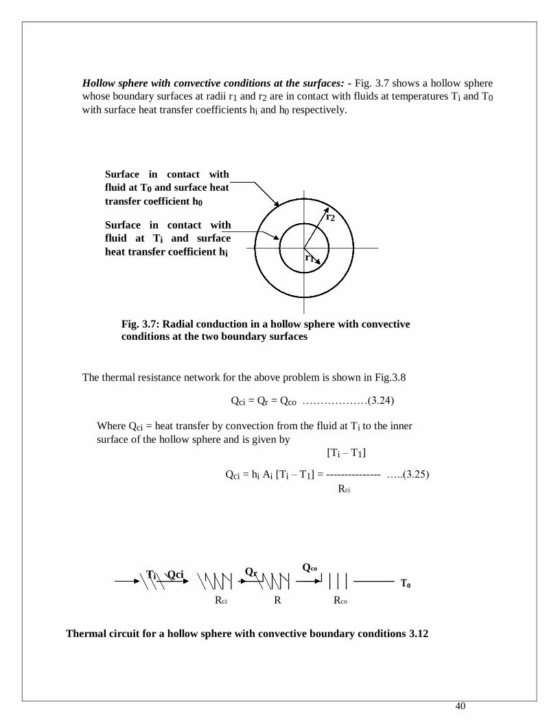
Hollow sphere with convective conditions at the surfaces: - Fig. 3.7 shows a hollow sphere

whose boundary surfaces at radii r1 and r2 are in contact with fluids at temperatures Ti and T0

with surface heat transfer coefficients hi and h0 respectively.

Surface in contact with

fluid at T0 and surface heat

transfer coefficient h0

Surface in contact with

fluid at Ti and surface

heat transfer coefficient hi

r2

r1

Fig. 3.7: Radial conduction in a hollow sphere with convective

conditions at the two boundary surfaces

The thermal resistance network for the above problem is shown in Fig.3.8

Qci = Qr = Qco ………………(3.24)

Where Qci = heat transfer by convection from the fluid at Ti to the inner

surface of the hollow sphere and is given by

[Ti – T1]

Qci = hi Ai [Ti – T1] = --------------- …..(3.25)

Rci

Ti Qci Qr

Qco

To

Rci R Rco

Thermal circuit for a hollow sphere with convective boundary conditions 3.12

41

When T1 = the inside surface temperature of the sphere and

Rci = 1 / (hiAi) = the thermal resistance for convection for the inside surface

Or Rci = 1 / (4 π r12 hi) ……………………………………………………….(3.25b)

Qr = Rate of heat transfer by conduction through the hollow sphere

= [T1 – T2] / R with R = (r2 – r1) / {4 π k r1 r2}

And Qco = Rate of heat transfer by convection from the outer surface of the sphere to

the outer fluid and is given by

[T2 – T0]

Qco = ho Ao [T2 – To] = --------------- ……………(3.26a)

Rco

Where T2 = outside surface temperature of the sphere and

Ao = outside surface area of the sphere = 4 π r22 so that

Rco = 1 / {4 π r22 ho}…………………………….(3.26b)

Now Eq.(3.24) can be written as

[Ti – T1] [T1 – T2] [T2 – T1]

Qr = hi Ai [Ti – T1] = -------------- = ---------------- = ----------------

Rci R Rco

Qr = ----------------------

[Ti – To]

…………………………………………(3.27)

[Rci + R + Rco]

Steady State conduction in composite medium:

There are many engineering applications in which heat transfer takes place through a

medium composed of several different layers, each having different thermal

conductivity. These layers may be arranged in series or in parallel or they may be

arranged with combined series-parallel arrangements. Such problems can be

conveniently solved using electrical analogy as illustrated in the following sections.

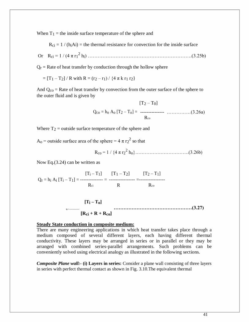
Composite Plane wall:- (i) Layers in series: Consider a plane wall consisting of three layers

in series with perfect thermal contact as shown in Fig. 3.10.The equivalent thermal

42

resistance network is also shown. If Q is the rate of heat transfer through an area A of the composite wall then we can write the expression for Q as follows:

Surface in

L1

L2 L3

contact Surface in contact with a fluid

with fluid

at T0 and surface heat

at Ti and

k1

k2

k3

transfer coefficient ho

surface

heat

transfer

coefficient

hi T1 T2 T3 T4

Rci R1 R2 R3 Rco

Q

Q

Ti T1 T2 T3 T4 To

A composite plane wall with three layers in series and the equivalent thermal

resistance network

(T2 – T3) (T1 – T2) (T1 – T2) (T2 – T3) (T3 – Tco) Q = -------------- = --------------- = ------------- = ------------ = ----------------

Rco R1 R2 R3 Rco

(Ti – T0) Ti – T0) Or Q = --------------------------------- = ------------…………………………….(3.28)

Rci + R1 + R2 + R3 + Rco Rtotal

Overall heat transfer coefficient for a composite wall: - It is sometimes convenient to

express the rate of heat transfer through a medium in a manner which is analogous to the Newton‟s law of cooling as follows:

If U is the overall heat transfer coefficient for the composite wall shown in Fig. (3.10) then

Q = U A (Ti – To) …………………………………...(3.29)

Comparing Eq. (3.28) with Eq. (3.29) we have the expression for U as

1 U = --------------- ……………………………………..(3.30)

A Rtotal

43

1 1

Or U = ------------------------------------= -----------------------------------------------------

A [ Rci + R1 + R2 + R3 ] A[1/(hiA) + L1/(Ak1) + L2/(Ak2) + L3/(Ak3)]

1

Or U = -------------------------------------------- ………………………………(3.31)

[ 1/hi + L1 / k1 + L2 / k2 + L3 / k3 ]

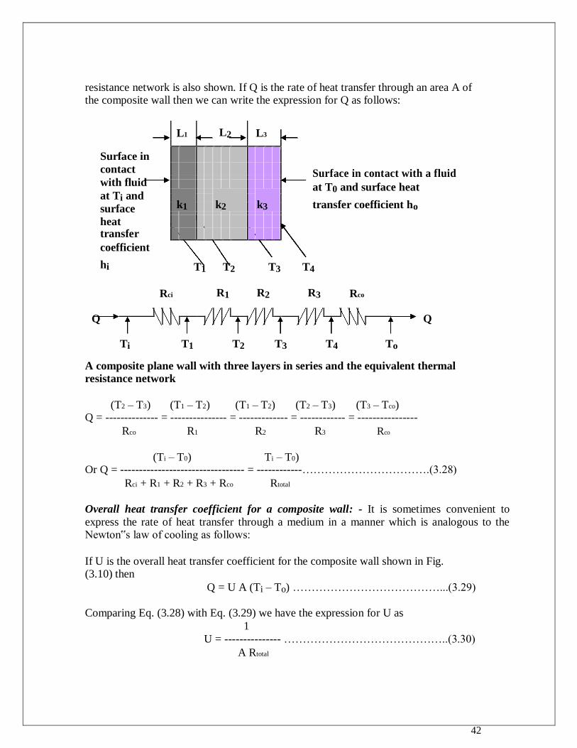
(ii) Layers in Parallel:- Fig.3.11 shows a composite plane wall in which three layers are

L

Surface in

k1

contact

with fluid

at Ti with k2

heat

transfer

coefficient

hi k3

Q1

Ti

T1

R1

Q2

Rci R2

Q3

R3

H1

H2

H3

Suface in contact

b with fluid at To and surface heat transfer

coefficient ho

T2

To

Rco

Q

Schematic and equivalent thermal circuit for a composite wall with layers in parallel

arranged in parallel. Let „b‟ be the dimension of these layers measured normal to the plane of the paper. Let one surface of the composite wall be in contact with a fluid at temperature

Ti and surface heat transfer coefficient hi and the other surface of the wall be in contact with

another fluid at temperature To with surface heat transfer coefficient ho. The equivalent thermal circuit for the composite wall is also shown in Fig. 3.11. The rate of heat transfer through the composite wall is given by

Q = Q1 + Q2 + Q3 ………………………….(3.32)

44

where Q1 = Rate of heat transfer through layer 1,

Q2 = Rate of heat transfer through layer 2, and

Q3 = Rate of heat transfer through layer 3.

(T1 – T2) Now Q1 = -------------- ……………………………………………………...(3.33a)

R1

Where R1 = {L / (H1bk1)}

Similarly Q2

(T1 – T2) = -------------- …………………………………………………(3.33b)

R2

Where R2

= {L / (H2bk2)}

(T1 – T2)

and Q3 = -------------- =

R3

……………………….. ………………………….(3.33c)

Where R3 = {L / (H3bk3)}

Substituting these expressions in Eq. (3.32) and simplifying we get

(T1 – T2) (T1 – T2) (T1 – T2) (T1 – T2) Q = ------------- + ---------------- + ----------------- = -------------------- ……….(3.34)

R1 R2 R3 Re

Where 1 / Re = 1/R1

+ 1/R2 + 1/R3

Hence Q =

(Ti – T1) (T1 – T2) (T2 – To) (Ti – To)

----------- = ------------ = ------------- = -------------------- …………(3.35) Rci Re Rco [Rci + Re + Rco]

Composite Coaxial Cylinders:- Fig. 3.12. shows a composite cylinder having two layers in series. The equivalent thermal circuit is also shown in the figure. The rate of heat

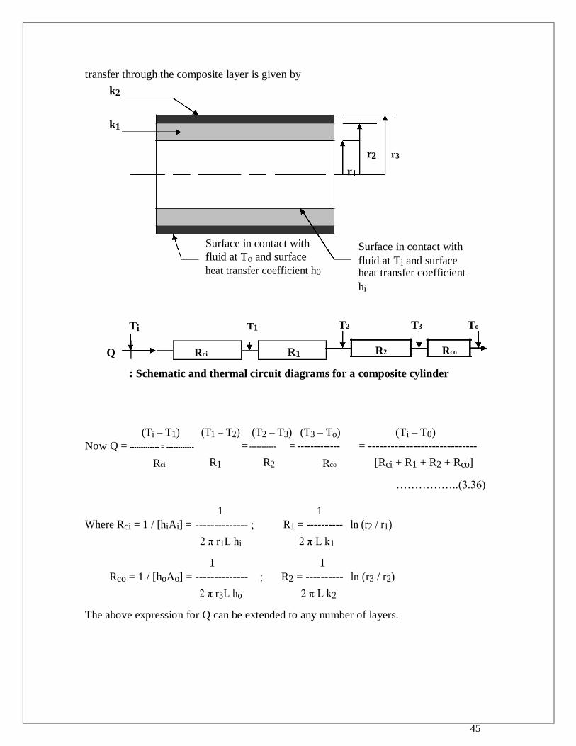
45

transfer through the composite layer is given by

k2

k1

Surface in contact with

fluid at To and surface

heat transfer coefficient h0

Ti T1

Q

Rci

R1

r2 r3

r1

Surface in contact with

fluid at Ti and surface heat transfer coefficient

hi

T2 T3 To

R2 Rco

: Schematic and thermal circuit diagrams for a composite cylinder

(Ti – T1) (T1 – T2) (T2 – T3) (T3 – To) (Ti – T0)

Now Q = ------------- = ------------ = ----------- = ------------- = -----------------------------

Rci R1 R2 Rco [Rci + R1 + R2 + Rco]

……………..(3.36)

1 1

Where Rci = 1 / [hiAi] = -------------- ; R1 = ---------- ln (r2 / r1)

2 π r1L hi 2 π L k1

1 1

Rco = 1 / [hoAo] = -------------- ; R2 = ---------- ln (r3 / r2)

2 π r3L ho 2 π L k2

The above expression for Q can be extended to any number of layers.

46

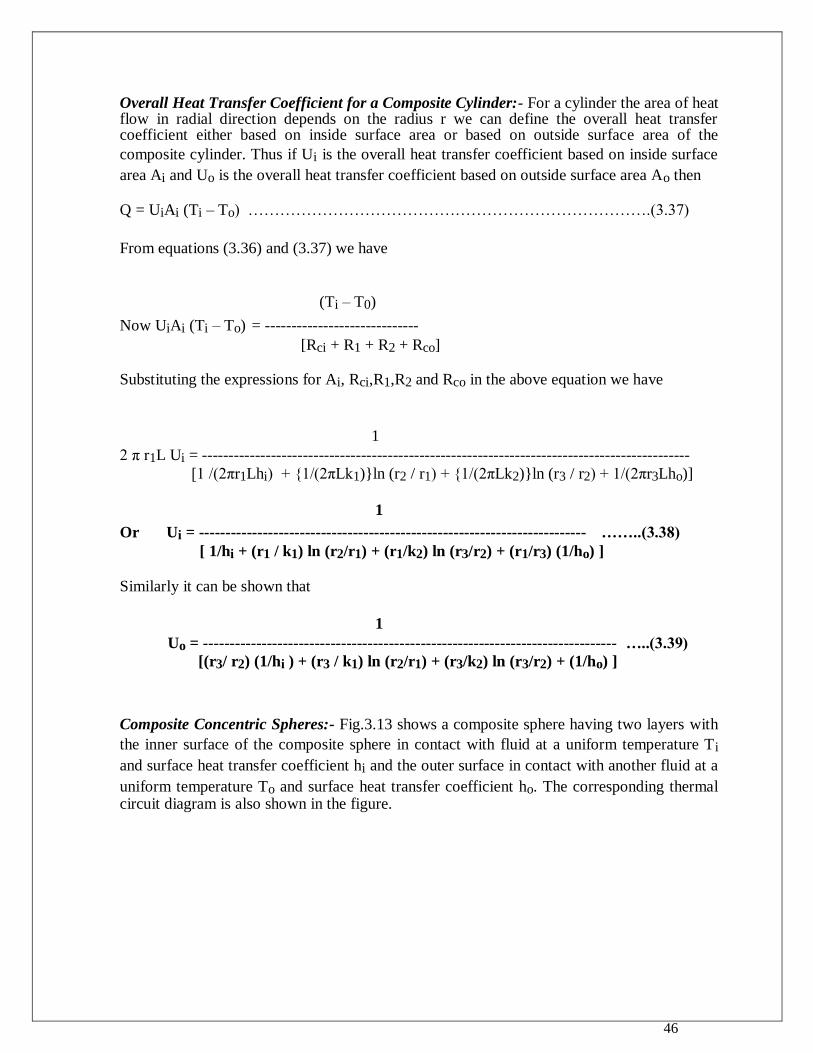
Overall Heat Transfer Coefficient for a Composite Cylinder:- For a cylinder the area of heat flow in radial direction depends on the radius r we can define the overall heat transfer coefficient either based on inside surface area or based on outside surface area of the

composite cylinder. Thus if Ui is the overall heat transfer coefficient based on inside surface

area Ai and Uo is the overall heat transfer coefficient based on outside surface area Ao then

Q = UiAi (Ti – To) ………………………………………………………………….(3.37)

From equations (3.36) and (3.37) we have

(Ti – T0)

Now UiAi (Ti – To) = -----------------------------

[Rci + R1 + R2 + Rco]

Substituting the expressions for Ai, Rci,R1,R2 and Rco in the above equation we have

1

2 π r1L Ui = --------------------------------------------------------------------------------------------

[1 /(2πr1Lhi) + {1/(2πLk1)}ln (r2 / r1) + {1/(2πLk2)}ln (r3 / r2) + 1/(2πr3Lho)]

1

Or Ui = ------------------------------------------------------------------------- ……..(3.38)

[ 1/hi + (r1 / k1) ln (r2/r1) + (r1/k2) ln (r3/r2) + (r1/r3) (1/ho) ]

Similarly it can be shown that

1

Uo = ------------------------------------------------------------------------------ …..(3.39)

[(r3/ r2) (1/hi ) + (r3 / k1) ln (r2/r1) + (r3/k2) ln (r3/r2) + (1/ho) ]

Composite Concentric Spheres:- Fig.3.13 shows a composite sphere having two layers with

the inner surface of the composite sphere in contact with fluid at a uniform temperature Ti

and surface heat transfer coefficient hi and the outer surface in contact with another fluid at a

uniform temperature To and surface heat transfer coefficient ho. The corresponding thermal circuit diagram is also shown in the figure.

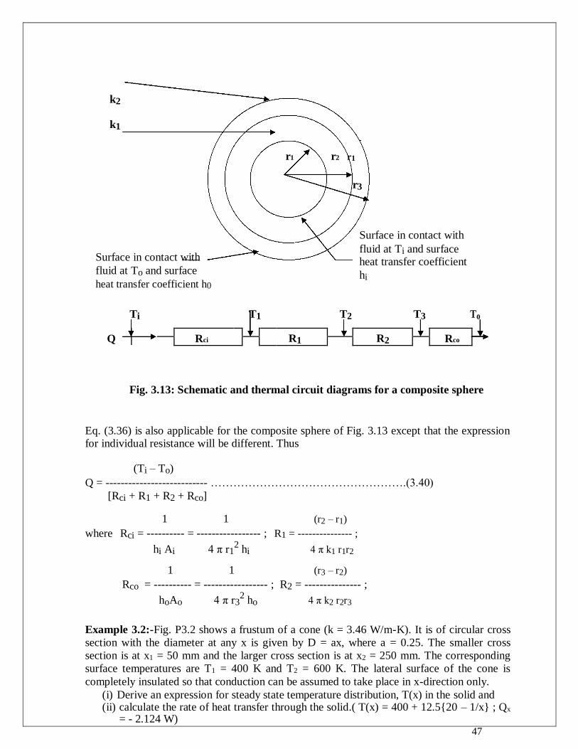
47

k2

k1

r1 r2 r1

r3

Surface in contact with

fluid at To and surface

heat transfer coefficient h0

Surface in contact with

fluid at Ti and surface

heat transfer coefficient

hi

Ti T1 T2 T3 To

Q

Rci

R1

R2

Rco

Fig. 3.13: Schematic and thermal circuit diagrams for a composite sphere

Eq. (3.36) is also applicable for the composite sphere of Fig. 3.13 except that the expression for individual resistance will be different. Thus

(Ti – To) Q = --------------------------- …………………………………………….(3.40)

[Rci + R1 + R2 + Rco]

1 1 (r2 – r1)

where Rci = ---------- = ----------------- ; R1 = --------------- ;

hi Ai 4 π r12 hi 4 π k1 r1r2

1 1 (r3 – r2)

Rco = ---------- = ----------------- ; R2 = --------------- ;

hoAo 4 π r32 ho 4 π k2 r2r3

Example 3.2:-Fig. P3.2 shows a frustum of a cone (k = 3.46 W/m-K). It is of circular cross

section with the diameter at any x is given by D = ax, where a = 0.25. The smaller cross

section is at x1 = 50 mm and the larger cross section is at x2 = 250 mm. The corresponding

surface temperatures are T1 = 400 K and T2 = 600 K. The lateral surface of the cone is

completely insulated so that conduction can be assumed to take place in x-direction only. (i) Derive an expression for steady state temperature distribution, T(x) in the solid and (ii) calculate the rate of heat transfer through the solid.( T(x) = 400 + 12.5{20 – 1/x} ; Qx

= - 2.124 W)

48

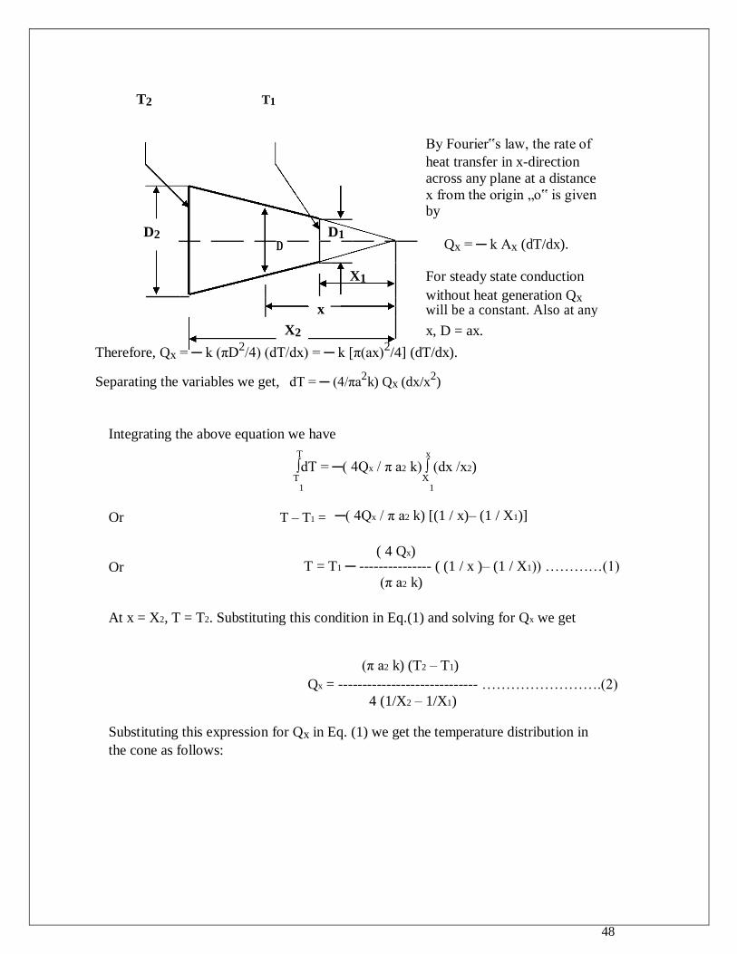
T2 T1

By Fourier‟s law, the rate of heat transfer in x-direction

across any plane at a distance x from the origin „o‟ is given

by

D2 D

D1 Qx = ─ k Ax (dT/dx).

X1

For steady state conduction

without heat generation Qx

x

will be a constant. Also at any

X2 x, D = ax.

Therefore, Qx = ─ k (πD2/4) (dT/dx) = ─ k [π(ax)

2/4] (dT/dx).

Separating the variables we get, dT = ─ (4/πa2k) Qx (dx/x

2)

Integrating the above equation we have

T x

∫dT = ─( 4Qx / π a2 k) ∫ (dx /x2) T X

1 1

Or

T – T1 =

─( 4Qx / π a2 k) [(1 / x)– (1 / X1)]

Or

( 4 Qx)

T = T1 ─ --------------- ( (1 / x )– (1 / X1)) …………(1) (π a2 k)

At x = X2, T = T2. Substituting this condition in Eq.(1) and solving for Qx we get

(π a2 k) (T2 – T1) Qx = ----------------------------- …………………….(2)

4 (1/X2 – 1/X1)

Substituting this expression for Qx in Eq. (1) we get the temperature distribution in

the cone as follows:

49

(T2 – T1) (1/x – 1/X1)

T(x) = T1 + --------------------------------- ………………..(3)

(1/X2 – 1/X1)

Substituting the given numerical values for X1, X2, T1 and T2 in Eq.(3) we get the

temperature distribution as follows:

(600 – 400) [ 1/ x – 1/0.05]

T(x) = 400 + ------------------------------------ [ 1/0.25 – 1/0.05}

Or T(x) = 400 + 12.5 [20 – 1/x]

Temperature distribution

π x (0.25)2 x 3.46 x [600 – 400]

And Qx = -------------------------------------------- = ─ 2.123 W

4 x [ 1/0.25 – 1/0.05 ]

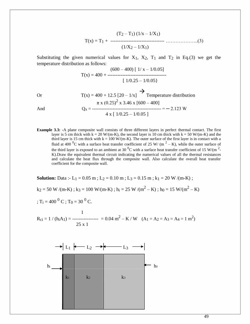
Example 3.3: -A plane composite wall consists of three different layers in perfect thermal contact. The first layer is 5 cm thick with k = 20 W/(m-K), the second layer is 10 cm thick with k = 50 W/(m-K) and the third layer is 15 cm thick with k = 100 W/(m-K). The outer surface of the first layer is in contact with a

fluid at 400 0C with a surface heat transfer coefficient of 25 W/ (m

2 – K), while the outer surface of

the third layer is exposed to an ambient at 30 0C with a surface heat transfer coefficient of 15 W/(m

2-

K).Draw the equivalent thermal circuit indicating the numerical values of all the thermal resistances and calculate the heat flux through the composite wall. Also calculate the overall heat transfer coefficient for the composite wall.

Solution: Data :- L1 = 0.05 m ; L2 = 0.10 m ; L3 = 0.15 m ; k1 = 20 W /(m-K) ;

k2 = 50 W /(m-K) ; k3 = 100 W/(m-K) ; hi = 25 W /(m2 – K) ; h0 = 15 W/(m

2 – K)

; Ti = 400 0 C ; T0 = 30

0 C.

1

Rci = 1 / (hiA1) = ---------------- = 0.04 m2 – K / W (A1 = A2 = A3 = A4 = 1 m2)

25 x 1

L1 L2 L3

hi

h0

k1 k2 k3

50

Q

Rci R1 R2 R3 R c0

0.05

= 0.0025 m2 – K / W.

R1 = L1 /(k1A1) = ---------------

20 x 1

----------------0.10

= 0.002 m2 – K / W.

R2 = L2 / (k2A2) =

50 x 1

------------------0.15

= 0.0015 m2 – K / W.

R3 = L3/ (k3A3) =

100 x 1

----------------1

= 0.067 m2 – K / W.

Rco = 1 / (h0A4) =

15 x 1

∑R = Rci + R1 + R2 + R3 + Rco = 0.04 + 0.0025 + 0.002 + 0.0015 + 0.067

Or ∑R = 0.113 m2-K/W.

(Ti – T0) (400 – 30)

Heat Flux through the composite slab = q = --------------- = ------------------

∑R 0.113

= 3274.34 W / m2.

If „U‟ is the overall heat transfer coefficient for the given system then

Q 1 1

U = ---------------- = ------------- = --------------

(Ti – T0) ∑R 0.113

= 8.85 W / (m2 – K).

51

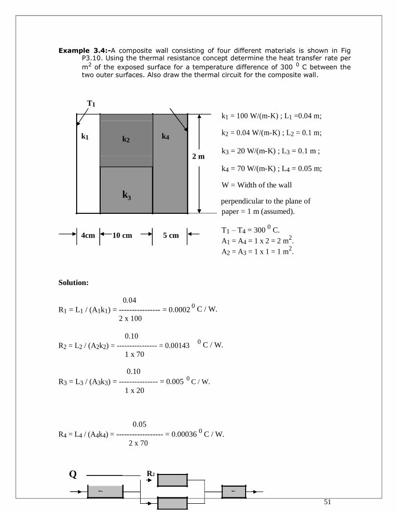
Example 3.4:-A composite wall consisting of four different materials is shown in Fig P3.10. Using the thermal resistance concept determine the heat transfer rate per

m2 of the exposed surface for a temperature difference of 300 0 C between the two outer surfaces. Also draw the thermal circuit for the composite wall.

T1

k1 = 100 W/(m-K) ; L1 =0.04 m;

k1 k2 k4

k2 = 0.04 W/(m-K) ; L2 = 0.1 m;

2 m

k3 = 20 W/(m-K) ; L3 = 0.1 m ;

k4 = 70 W/(m-K) ; L4 = 0.05 m;

W = Width of the wall

k3 perpendicular to the plane of

paper = 1 m (assumed).

4cm

10 cm

5 cm

T1 – T4 = 300 0 C.

A1 = A4 = 1 x 2 = 2 m2.

Solution:

A2 = A3 = 1 x 1 = 1 m2.

0.04 0 C / W.

R1 = L1 / (A1k1) = ---------------- = 0.0002

2 x 100

0.10 0 C / W.

R2 = L2 / (A2k2) = ---------------- = 0.00143

1 x 70

0.10

R3 = L3 / (A3k3) = --------------- = 0.005 0

C / W.

1 x 20

0.05

R4 = L4 / (A4k4) = ------------------ = 0.00036 0 C / W.

2 x 70

Q R2

R1

R4

52

R3

Thermal potential = T1 – T4

R2 and R3 are resistances in parallel and they can be replaced by a

single equivalent resistance Re, where

R2 R3 0.00143 x 0.005

1 / Re = 1 / R2 + 1 / R3 or Re = --------------- = ----------------------- = 0.0011 0C/W

(R2 + R3) (0.00143 + 0.005)

Now R1, Re and R4 are resistances in series so that

(T1 – T4) ----------------------- ------------- 300

= 86.705 x 103 W

Q = --------------------- =

(R1 + Re + R4) [0.002 + 0.0011 + 0.00036]

Heat transfer per unit area of the exposed surface is given by

q = Q / A1 = 86.705 / 2.0 = 43.35 kW.

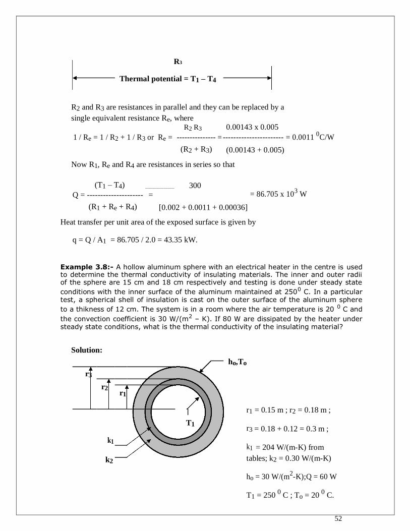
Example 3.8:- A hollow aluminum sphere with an electrical heater in the centre is used to determine the thermal conductivity of insulating materials. The inner and outer radii of the sphere are 15 cm and 18 cm respectively and testing is done under steady state

conditions with the inner surface of the aluminum maintained at 2500 C. In a particular test, a spherical shell of insulation is cast on the outer surface of the aluminum sphere

to a thikness of 12 cm. The system is in a room where the air temperature is 20 0 C and

the convection coefficient is 30 W/(m2 – K). If 80 W are dissipated by the heater under steady state conditions, what is the thermal conductivity of the insulating material?

Solution:

ho,To

r3

r2

r1

r1 = 0.15 m ; r2 = 0.18 m ;

T1 r3 = 0.18 + 0.12 = 0.3 m ;

k1 k1 = 204 W/(m-K) from

k2

tables; k2 = 0.30 W/(m-K)

ho = 30 W/(m2-K);Q = 60 W

T1 = 250 0 C ; To = 20

0 C.

53

(r2 – r1) (0.18 – 0.15)

R1 = ---------------- = ------------------------------ = 4.335 x 10 ─ 4

0 C / W.

4π k1 r1 r2 4 π x 204 x 0.18 x 0.15

(r3 – r2) (0.30 – 0.18)

R2 = ---------------- = ------------------------------ = 0.177 / k2 0 C / W.

4π k2 r2 r3 4 π x k2 x 0.30 x 0.18

1 1

Rco = 1 / (hoAo) = ------------------- = --------------------- = 0.0295

4π r32 ho 4π x (0.3)

2 x 30

(T1 – To)

Q = -------------------- or R2 = (T1 – To) / Q – (R1 + Rco)

R1 + R2 + Rco Or R2 = (250 – 20) / 80 ─ (4.335 x 10

─ 4

Therefore 0.177 / k2 = 2.845

0 C / W.

+ 0.0295) = 2.874

Or k2 = 0.177 / 2.845 = 0.062 W / (m-K)

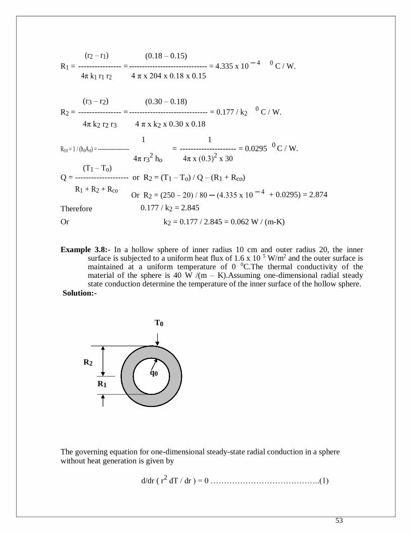
Example 3.8:- In a hollow sphere of inner radius 10 cm and outer radius 20, the inner

surface is subjected to a uniform heat flux of 1.6 x 10 5 W/m2 and the outer surface is maintained at a uniform temperature of 0 0C.The thermal conductivity of the material of the sphere is 40 W /(m – K).Assuming one-dimensional radial steady state conduction determine the temperature of the inner surface of the hollow sphere.

Solution:-

T0

R2

q0

R1

The governing equation for one-dimensional steady-state radial conduction in a sphere without heat generation is given by

d/dr ( r2 dT / dr ) = 0 …………………………………..(1)

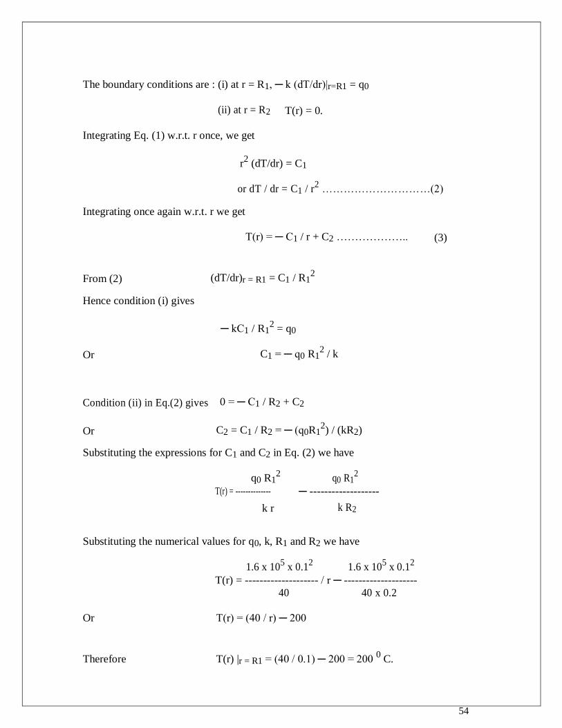
54

The boundary conditions are : (i) at r = R1, ─ k (dT/dr)|r=R1 = q0

(ii) at r = R2 T(r) = 0.

Integrating Eq. (1) w.r.t. r once, we get

r2 (dT/dr) = C1

or dT / dr = C1 / r2 …………………………(2)

Integrating once again w.r.t. r we get

T(r) = ─ C1 / r + C2 ……………….. (3)

From (2) (dT/dr)r = R1 = C1 / R12

Hence condition (i) gives

─ kC1 / R12 = q0

Or C1 = ─ q0 R12 / k

Condition (ii) in Eq.(2) gives 0 = ─ C1 / R2 + C2

Or C2 = C1 / R2 = ─ (q0R12) / (kR2)

Substituting the expressions for C1 and C2 in Eq. (2) we have

q0 R12 q0 R1

2

T(r) = -------------- ─ -------------------

k r k R2

Substituting the numerical values for q0, k, R1 and R2 we have

1.6 x 105 x 0.1

2 1.6 x 10

5 x 0.1

2

T(r) = -------------------- / r ─ --------------------

40 40 x 0.2

Or T(r) = (40 / r) ─ 200

Therefore T(r) |r = R1 = (40 / 0.1) ─ 200 = 200 0 C.

55

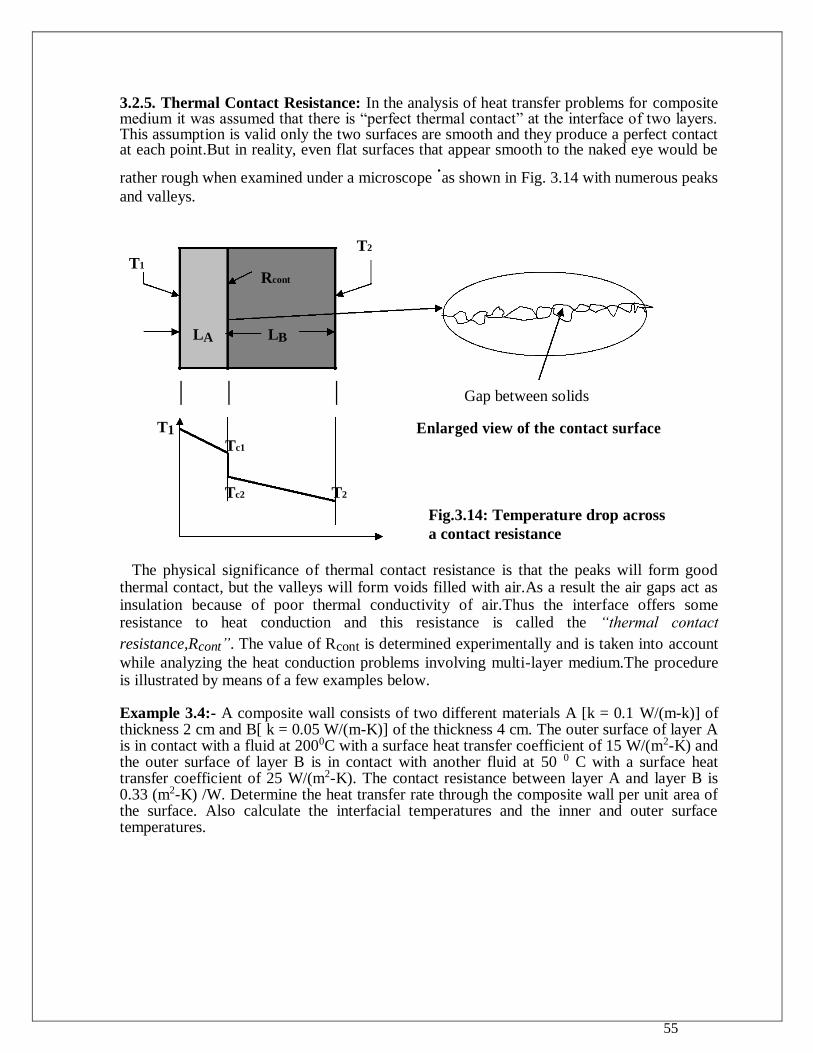
3.2.5. Thermal Contact Resistance: In the analysis of heat transfer problems for composite medium it was assumed that there is “perfect thermal contact” at the interface of two layers. This assumption is valid only the two surfaces are smooth and they produce a perfect contact at each point.But in reality, even flat surfaces that appear smooth to the naked eye would be

rather rough when examined under a microscope .as shown in Fig. 3.14 with numerous peaks

and valleys.

T2 T1

Rcont

LA LB

Gap between solids

T1 Enlarged view of the contact surface

Tc1

Tc2 T2

Fig.3.14: Temperature drop across a contact resistance

The physical significance of thermal contact resistance is that the peaks will form good thermal contact, but the valleys will form voids filled with air.As a result the air gaps act as insulation because of poor thermal conductivity of air.Thus the interface offers some resistance to heat conduction and this resistance is called the “thermal contact

resistance,Rcont”. The value of Rcont is determined experimentally and is taken into account

while analyzing the heat conduction problems involving multi-layer medium.The procedure is illustrated by means of a few examples below.

Example 3.4:- A composite wall consists of two different materials A [k = 0.1 W/(m-k)] of thickness 2 cm and B[ k = 0.05 W/(m-K)] of the thickness 4 cm. The outer surface of layer A is in contact with a fluid at 2000C with a surface heat transfer coefficient of 15 W/(m2-K) and the outer surface of layer B is in contact with another fluid at 50 0 C with a surface heat transfer coefficient of 25 W/(m2-K). The contact resistance between layer A and layer B is 0.33 (m2-K) /W. Determine the heat transfer rate through the composite wall per unit area of the surface. Also calculate the interfacial temperatures and the inner and outer surface temperatures.

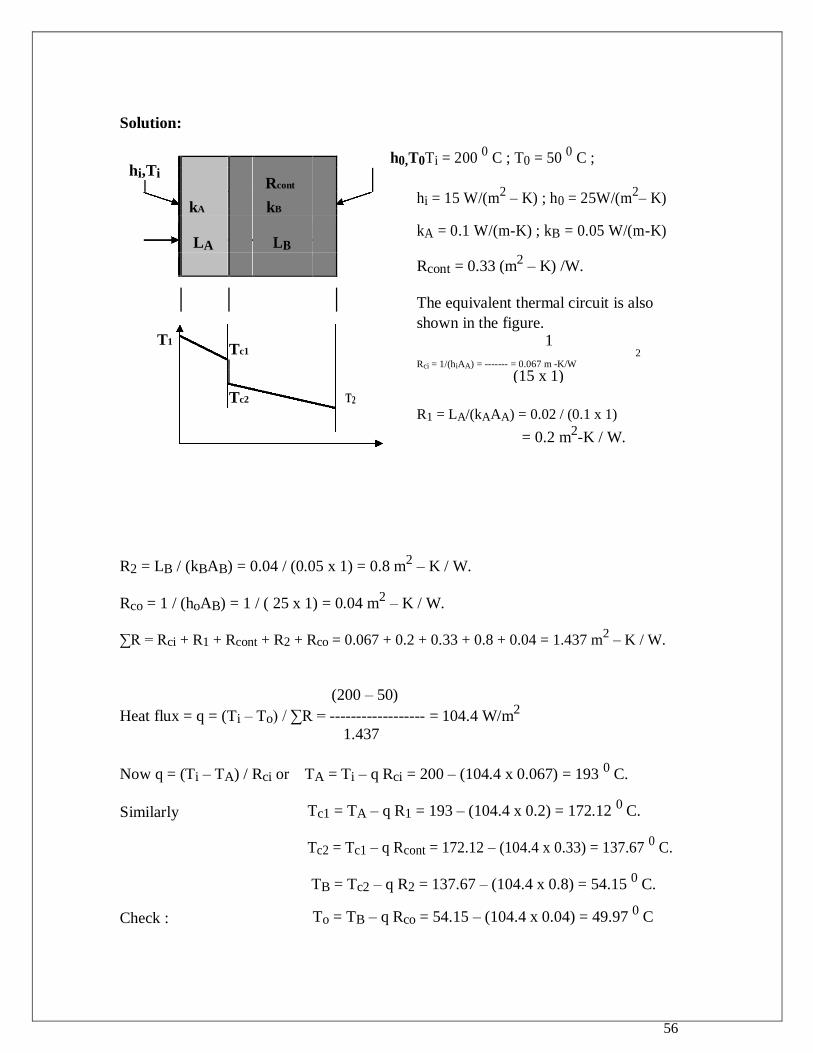
56

Solution:

hi,Ti

h0,T0Ti = 200

0 C ; T0 = 50

0 C ;

Rcont

hi = 15 W/(m2 – K) ; h0 = 25W/(m

2– K)

kA

kB

LA

LB

kA = 0.1 W/(m-K) ; kB = 0.05 W/(m-K)

Rcont = 0.33 (m2 – K) /W.

The equivalent thermal circuit is also

T1

shown in the figure.

Tc1

1

2

Rci = 1/(hiAA) = ------- = 0.067 m -K/W

(15 x 1)

Tc2 T2

R1 = LA/(kAAA) = 0.02 / (0.1 x 1)

= 0.2 m2-K / W.

R2 = LB / (kBAB) = 0.04 / (0.05 x 1) = 0.8 m2 – K / W.

Rco = 1 / (hoAB) = 1 / ( 25 x 1) = 0.04 m2 – K / W.

∑R = Rci + R1 + Rcont + R2 + Rco = 0.067 + 0.2 + 0.33 + 0.8 + 0.04 = 1.437 m2 – K / W.

(200 – 50)

Heat flux = q = (Ti – To) / ∑R = ------------------ = 104.4 W/m2

1.437

Now q = (Ti – TA) / Rci or TA = Ti – q Rci = 200 – (104.4 x 0.067) = 193 0 C.

Similarly Tc1 = TA – q R1 = 193 – (104.4 x 0.2) = 172.12 0 C.

Tc2 = Tc1 – q Rcont = 172.12 – (104.4 x 0.33) = 137.67 0 C.

TB = Tc2 – q R2 = 137.67 – (104.4 x 0.8) = 54.15 0 C.

Check : To = TB – q Rco = 54.15 – (104.4 x 0.04) = 49.97 0 C

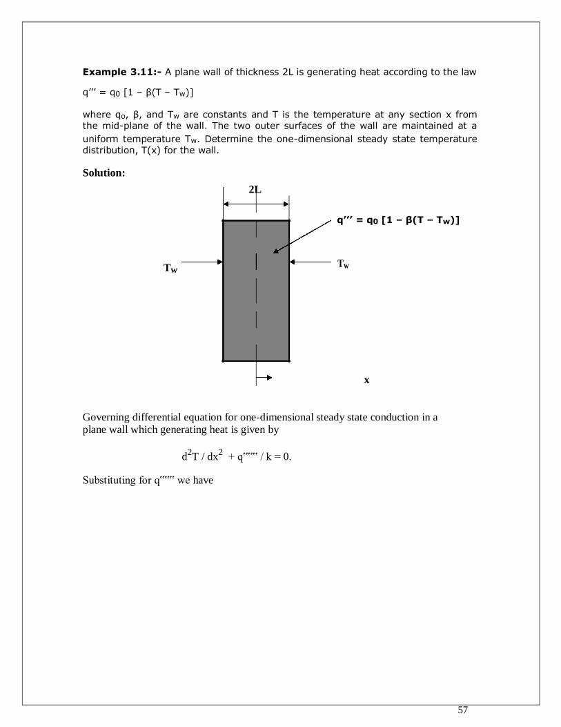
57

Example 3.11:- A plane wall of thickness 2L is generating heat according to the law

q’’’ = q0 [1 – β(T – Tw)]

where qo, β, and Tw are constants and T is the temperature at any section x from the mid-plane of the wall. The two outer surfaces of the wall are maintained at a

uniform temperature Tw. Determine the one-dimensional steady state temperature distribution, T(x) for the wall.

Solution:

2L

q’’’ = q0 [1 – β(T – Tw)]

Tw Tw

x

Governing differential equation for one-dimensional steady state conduction in a plane wall which generating heat is given by

d2T / dx

2 + q‟‟‟ / k = 0.

Substituting for q‟‟‟ we have

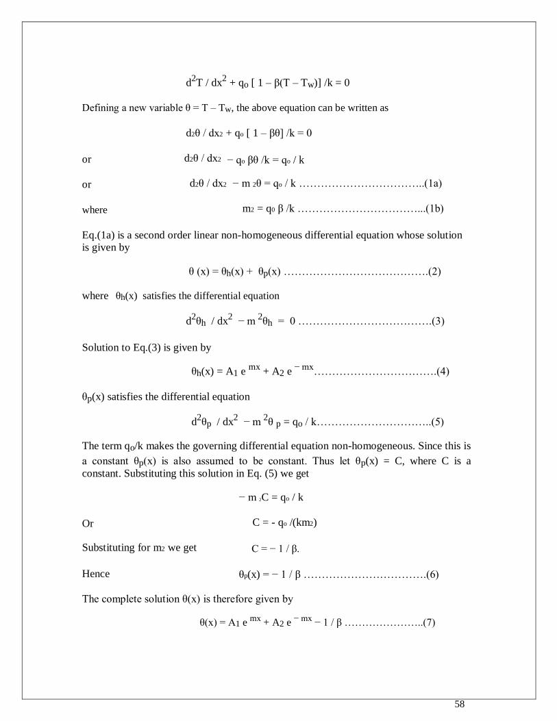
58

d2T / dx

2 + qo [ 1 – β(T – Tw)] /k = 0

Defining a new variable θ = T – Tw, the above equation can be written as

d2θ / dx2 + qo [ 1 – βθ] /k = 0

or

d2θ / dx2

− qo βθ /k = qo / k

or d2θ / dx2

− m 2θ = qo / k ……………………………..(1a)

where

m2 = q0 β /k ……………………………...(1b)

Eq.(1a) is a second order linear non-homogeneous differential equation whose solution is given by

θ (x) = θh(x) + θp(x) ………………………………….(2)

where θh(x) satisfies the differential equation

d2θh / dx

2 − m

2θh = 0 ……………………………….(3)

Solution to Eq.(3) is given by

θh(x) = A1 e mx

+ A2 e − mx

…………………………….(4)

θp(x) satisfies the differential equation

d2θp / dx

2 − m

2θ p = qo / k…………………………..(5)

The term qo/k makes the governing differential equation non-homogeneous. Since this is

a constant θp(x) is also assumed to be constant. Thus let θp(x) = C, where C is a

constant. Substituting this solution in Eq. (5) we get

− m 2C = qo / k

Or

C = - qo /(km2)

Substituting for m2 we get

C = − 1 / β.

Hence

θp(x) = − 1 / β …………………………….(6)

The complete solution θ(x) is therefore given by

θ(x) = A1 e mx + A2 e − mx − 1 / β …………………..(7)

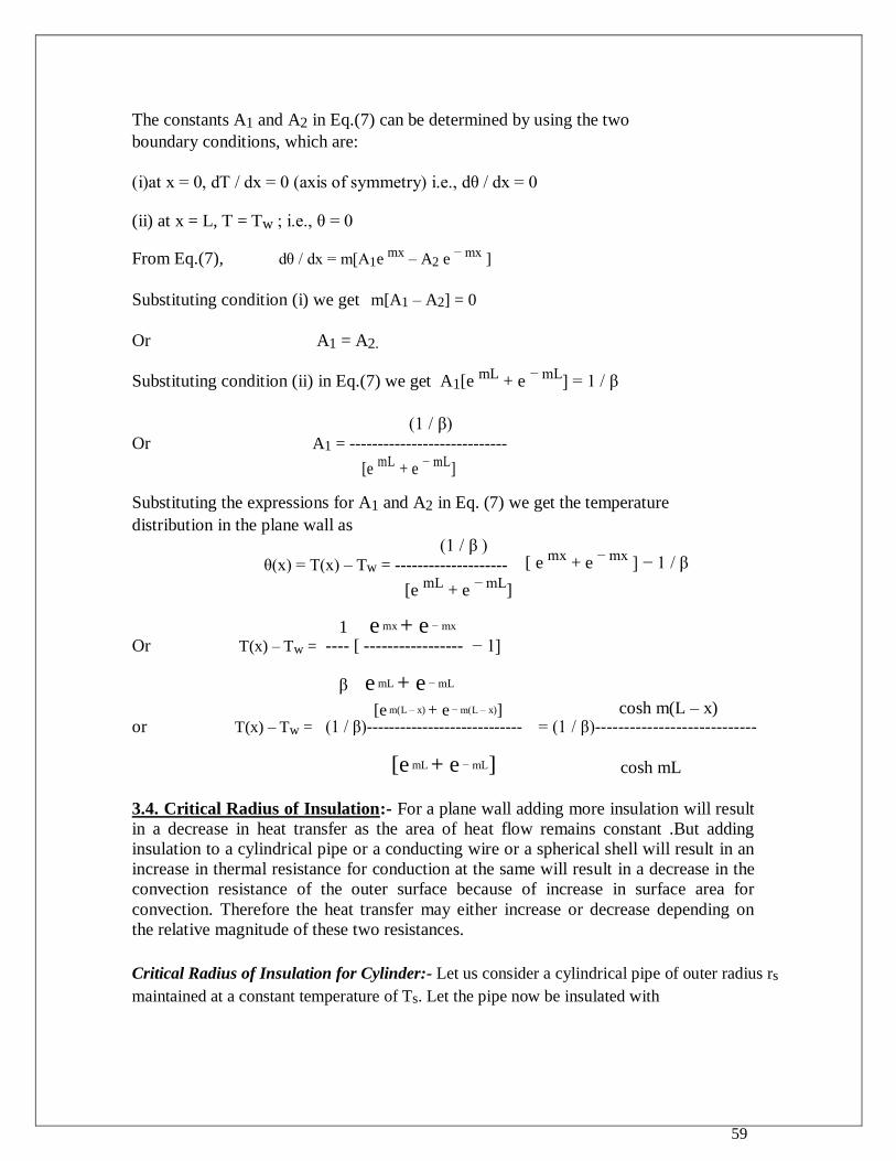
59

The constants A1 and A2 in Eq.(7) can be determined by using the two

boundary conditions, which are:

(i)at x = 0, dT / dx = 0 (axis of symmetry) i.e., dθ / dx = 0

(ii) at x = L, T = Tw ; i.e., θ = 0

From Eq.(7), dθ / dx = m[A1e mx

– A2 e − mx

]

Substituting condition (i) we get m[A1 – A2] = 0

Or A1 = A2.

Substituting condition (ii) in Eq.(7) we get A1[e mL

+ e − mL

] = 1 / β

(1 / β) Or A1 = ----------------------------

[e mL

+ e − mL

]

Substituting the expressions for A1 and A2 in Eq. (7) we get the temperature

distribution in the plane wall as

(1 / β ) [ e

mx + e

− mx ] − 1 / β

θ(x) = T(x) – Tw = --------------------

[e mL

+ e − mL

]

1 e mx + e − mx

Or T(x) – Tw = ---- [ ----------------- − 1]

β e mL + e − mL

[e m(L – x) + e − m(L – x)] cosh m(L – x)

or T(x) – Tw = (1 / β)---------------------------- = (1 / β)----------------------------

[e mL + e − mL] cosh mL

3.4. Critical Radius of Insulation:- For a plane wall adding more insulation will result

in a decrease in heat transfer as the area of heat flow remains constant .But adding

insulation to a cylindrical pipe or a conducting wire or a spherical shell will result in an

increase in thermal resistance for conduction at the same will result in a decrease in the

convection resistance of the outer surface because of increase in surface area for

convection. Therefore the heat transfer may either increase or decrease depending on

the relative magnitude of these two resistances.

Critical Radius of Insulation for Cylinder:- Let us consider a cylindrical pipe of outer radius rs

maintained at a constant temperature of Ts. Let the pipe now be insulated with

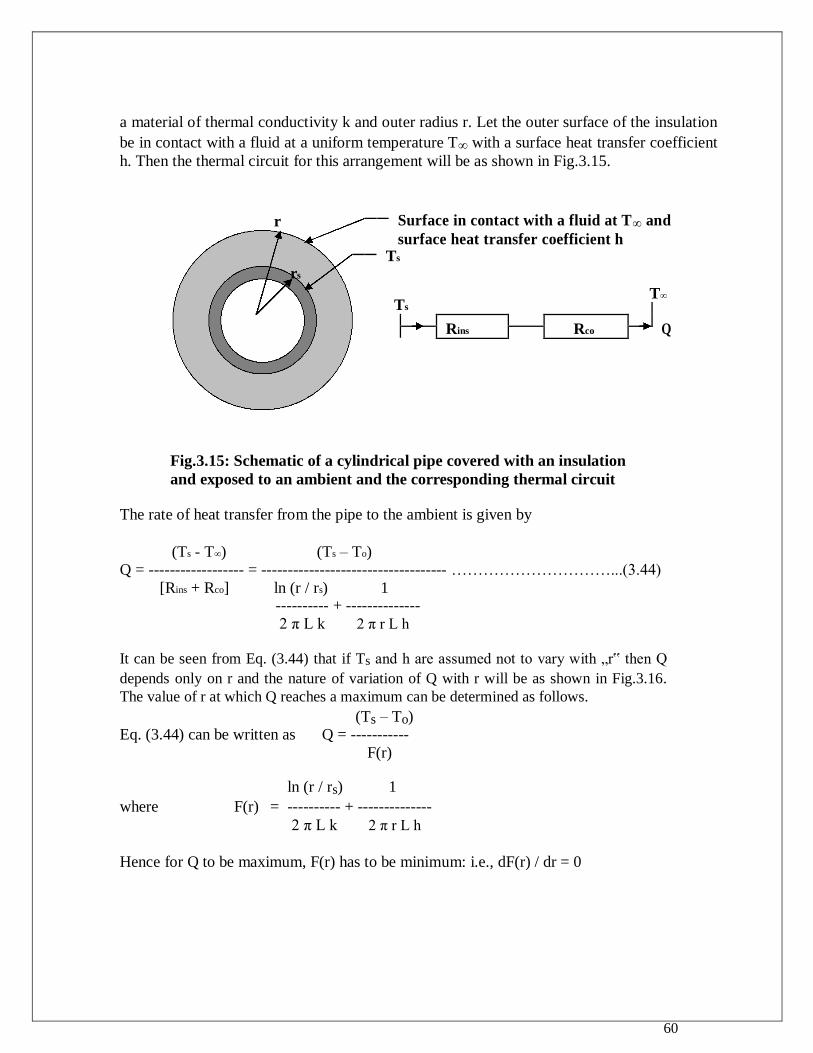
60

a material of thermal conductivity k and outer radius r. Let the outer surface of the insulation

be in contact with a fluid at a uniform temperature T∞ with a surface heat transfer coefficient

h. Then the thermal circuit for this arrangement will be as shown in Fig.3.15.

r

Surface in contact with a fluid at T∞ and

surface heat transfer coefficient h

Ts

rs

Ts

T∞

Rins

Rco

Q

Fig.3.15: Schematic of a cylindrical pipe covered with an insulation

and exposed to an ambient and the corresponding thermal circuit

The rate of heat transfer from the pipe to the ambient is given by

(Ts - T∞) (Ts – To) Q = ------------------ = ----------------------------------- …………………………...(3.44)

[Rins + Rco] ln (r / rs) 1

---------- + --------------

2 π L k 2 π r L h

It can be seen from Eq. (3.44) that if Ts and h are assumed not to vary with „r‟ then Q

depends only on r and the nature of variation of Q with r will be as shown in Fig.3.16.

The value of r at which Q reaches a maximum can be determined as follows.

(Ts – To) Eq. (3.44) can be written as Q = -----------

F(r)

ln (r / rs) 1 where F(r) = ---------- + --------------

2 π L k 2 π r L h

Hence for Q to be maximum, F(r) has to be minimum: i.e., dF(r) / dr = 0

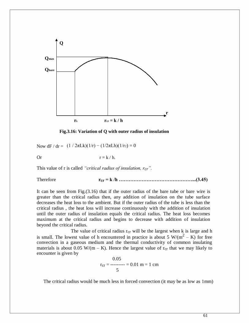
61

Q

Qmax

Qbare

r

rs rcr = k / h

Fig.3.16: Variation of Q with outer radius of insulation

Now dF / dr =

(1 / 2πLk)(1/r) − (1/2πLh)(1/r2) = 0

Or

r = k / h.

This value of r is called “critical radius of insulation, rcr”.

Therefore rcr = k /h ………………………………………...(3.45)

It can be seen from Fig.(3.16) that if the outer radius of the bare tube or bare wire is

greater than the critical radius then, any addition of insulation on the tube surface

decreases the heat loss to the ambient. But if the outer radius of the tube is less than the

critical radius , the heat loss will increase continuously with the addition of insulation

until the outer radius of insulation equals the critical radius. The heat loss becomes

maximum at the critical radius and begins to decrease with addition of insulation

beyond the critical radius.

The value of critical radius rcr will be the largest when k is large and h

is small. The lowest value of h encountered in practice is about 5 W/(m2 – K) for free

convection in a gaseous medium and the thermal conductivity of common insulating

materials is about 0.05 W/(m – K). Hence the largest value of rcr that we may likely to encounter is given by

0.05

rcr = --------- = 0.01 m = 1 cm

5

The critical radius would be much less in forced convection (it may be as low as 1mm)

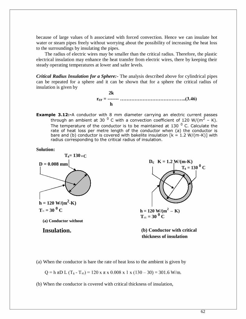
62

because of large values of h associated with forced convection. Hence we can insulate hot

water or steam pipes freely without worrying about the possibility of increasing the heat loss to the surroundings by insulating the pipes.

The radius of electric wires may be smaller than the critical radius. Therefore, the plastic

electrical insulation may enhance the heat transfer from electric wires, there by keeping their steady operating temperatures at lower and safer levels.

Critical Radius Insulation for a Sphere:- The analysis described above for cylindrical pipes

can be repeated for a sphere and it can be shown that for a sphere the critical radius of insulation is given by

2k

rcr = ------- …………………………………..(3.46)

h

Example 3.12:-A conductor with 8 mm diameter carrying an electric current passes

through an ambient at 30 0 C with a convection coefficient of 120 W/(m2 – K).

The temperature of the conductor is to be maintained at 130 0 C. Calculate the rate of heat loss per metre length of the conductor when (a) the conductor is bare and (b) conductor is covered with bakelite insulation [k = 1.2 W/(m-K)] with radius corresponding to the critical radius of insulation.

Solution:

Ts= 130 0 C

D = 0.008 mm

Dc K = 1.2 W/(m-K)

Ts = 130 0 C

h = 120 W/(m2-K)

T∞ = 30 0 C h = 120 W/(m

2 – K)

T∞ = 30 0 C

(a) Conductor without

Insulation. (b) Conductor with critical

thickness of insulation

(a) When the conductor is bare the rate of heat loss to the ambient is given by

Q = h πD L (Ts - T∞) = 120 x π x 0.008 x 1 x (130 – 30) = 301.6 W/m.

(b) When the conductor is covered with critical thickness of insulation,

63

Dc = 2 rc = 2 (k/h) = 2 x ( 1.2 / 120) = 0.02 m.

1 1

R insulation = -------------- ln (Dc / D) = ----------------------- ln (0.02 / 0.008)

2π L k 2 π x 1.0 x 1.2

= 0.1215 (m – 0 C) / W.

1 1

Rco = 1 / (h Ac) = ---------------- = ------ ---- ---- ---- ---- -- = 0.133 (m –

0 C)/W.

π Dc L h π x 0.02 x 1 x 120

∑R = Rinsulation + Rco = 0.1215 + 0.133 = 0.2545 (m – 0 C) / W.

(Ts - T∞) (130 – 30)

Qinsulation = ------------------- = --------------- = 392.93 W / m. ∑R 0.145

Example 3.13: -An electrical current of 700 A flows through a stainless steel cable

having a diameter of 5 mm and an electrical resistance of 6x10 ─ 4

ohms per metre length of the cable. The cable is in an environment

at a uniform temperature of 30 0 C and the surface heat transfer

coefficient of 25 W/(m2 – 0C).

(a) What is the surface temperature of the cable when it is bare? (b)What thickness of insulation of k = 0.5 W/(m – K) will yield the lowest value of the maximum insulation temperature? What is this temperature when the thickness is used?

Solution: (a) When the cable is Bare: - Electrical Resistance = Re = 6 x 10 ─ 4

Ω / m

Current through the cable = I = 700 A; D = 0.005 m ; h = 25 W/(m2-K) ; T∞ = 30

0

C. Power dissipated = Q = I2 Re = (700)

2 x 6 x 10

─ 4 = 294 W / m.

But Q = hA(Ts - T∞) or Ts = T∞ + Q / [(πD L) x h]

Or Ts = 30 + 294 / [(π x 0.005 x 1) x 25] = 779 0 C.

(b) When the cable is covered with insulation:

k = 0.5 W/(m-K) ; Hence critical radius = rc = k / h = 0.5 / 25 = 0.02 (m-K) /

W. Thickness of insulation = rc – D/2 = 0.02 – 0.005 / 2 = 0.0175 m

64

1 1 Rinsulation = --------------- ln (rc / ro) = ------------------- ln (0.02 / 0.0025) = 0.662 (m-K)/W

(2π L k) (2π x 1 x 0.5)

1 1 Rco = 1 / (hAo) = ------------------- = ------------------------------ = 0.318 (m-K) / W.

(2π rcL h) (2 x π x 0.02 x 1 x 25)

(Ts - T∞) Q = ---------------------

or

Ts = T∞ + Q (Rinsulation + Rco)

Rinsulation + Rco

Or

Ts = 30 + 294 x (0.662 + 0.318)

= 318.12 0 C.

Example 3.14:- A 2 mm-diameter and 10 m-long electric wire is tightly wrapped With a 1 mm-thick plastic cover whose thermal conductivity is 0.15 W / (m-K). Electrical measurements indicate that a current of 10 A passes through the wire and there is a

voltage drop of 8 V along the wire. If the insulated wire is exposed to a medium at 30 0C

with a heat transfer coefficient of 24 W / (m2 – K), determine the temperature at the

interface of the wire and the plastic cover in steady operation. Also determine if doubling the thickness of the plastic cover will increase or decrease this interface temperature.

Given: Outer radius of the bare wire = rs = 1 mm = 0.001 m ; Length of the wire = L = 10 m

; outer radius of plastic insulation = r = 1 + 1 = 2 mm = 0.002 m ; Current through the wire = I = 10 A ; Voltage drop in the wire = V = 8 V ; Ambient

temperature = T∞ = 30 0C ; Thermal conductivity of the plastic cover = k = 0.15 W /(m– K) ;

Surface heat transfer coefficient = h = 24 W /(m2 – K).

To find: (i) Interface temperature = Ts ; (ii) Whether Ts increases or decreases when

the thickness of insulation is doubled.

Solution: (i) Q = VI = 8 x 10 = 80 W.

The thermal circuit for the problem is shown in Fig. P3.14.

ln (r / rs) ln ( 0.002 / 0.001)

Rins = ------------ = ----------------------------- = 0.0735 K / W

2 π L k 2 x π x 10 x 0.15

1 1 1 Rco = -------------- = -------------- = ------------------------------ = 0.3316 K / W

h Ao 2 π L r h 2 x π x 10 x 0.002 x 24

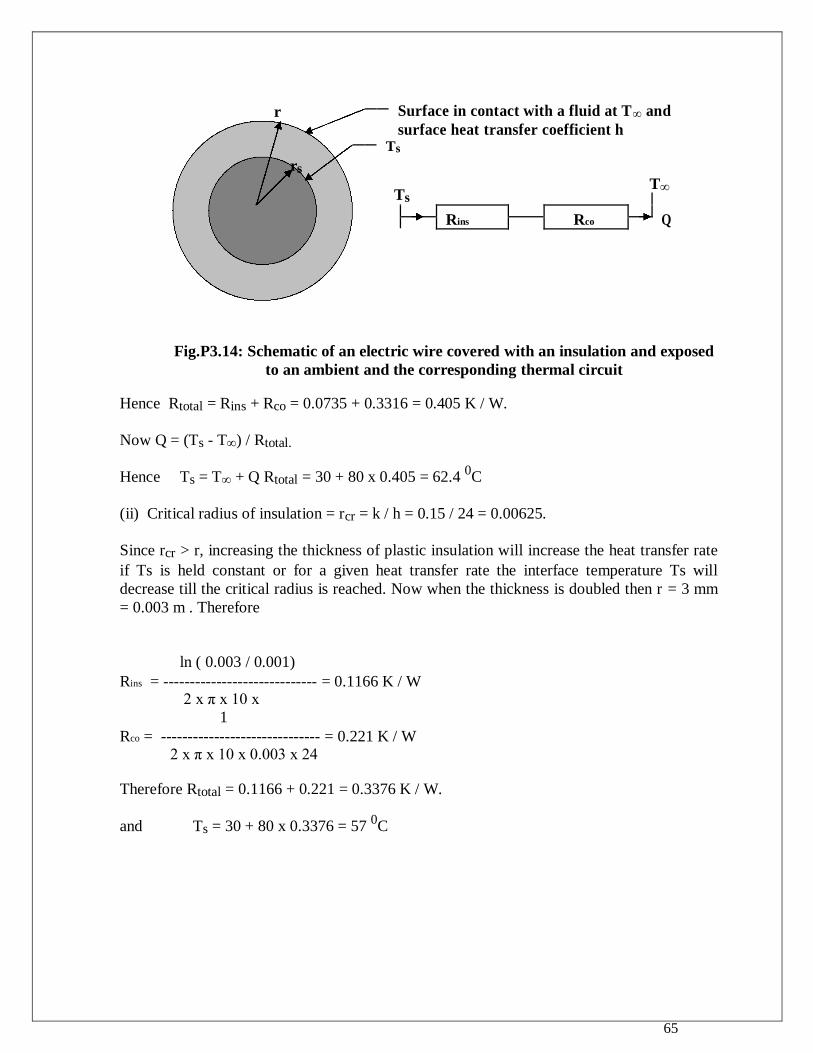
65

r

Surface in contact with a fluid at T∞ and

surface heat transfer coefficient h

Ts

rs

Ts

T∞

Rins

Rco

Q

Fig.P3.14: Schematic of an electric wire covered with an insulation and exposed

to an ambient and the corresponding thermal circuit

Hence Rtotal = Rins + Rco = 0.0735 + 0.3316 = 0.405 K / W.

Now Q = (Ts - T∞) / Rtotal.

Hence Ts = T∞ + Q Rtotal = 30 + 80 x 0.405 = 62.4 0C

(ii) Critical radius of insulation = rcr = k / h = 0.15 / 24 = 0.00625.

Since rcr > r, increasing the thickness of plastic insulation will increase the heat transfer rate

if Ts is held constant or for a given heat transfer rate the interface temperature Ts will

decrease till the critical radius is reached. Now when the thickness is doubled then r = 3 mm

= 0.003 m . Therefore

ln ( 0.003 / 0.001) Rins = ----------------------------- = 0.1166 K / W

2 x π x 10 x 1

Rco = ------------------------------ = 0.221 K / W

2 x π x 10 x 0.003 x 24

Therefore Rtotal = 0.1166 + 0.221 = 0.3376 K / W.

and Ts = 30 + 80 x 0.3376 = 57 0C

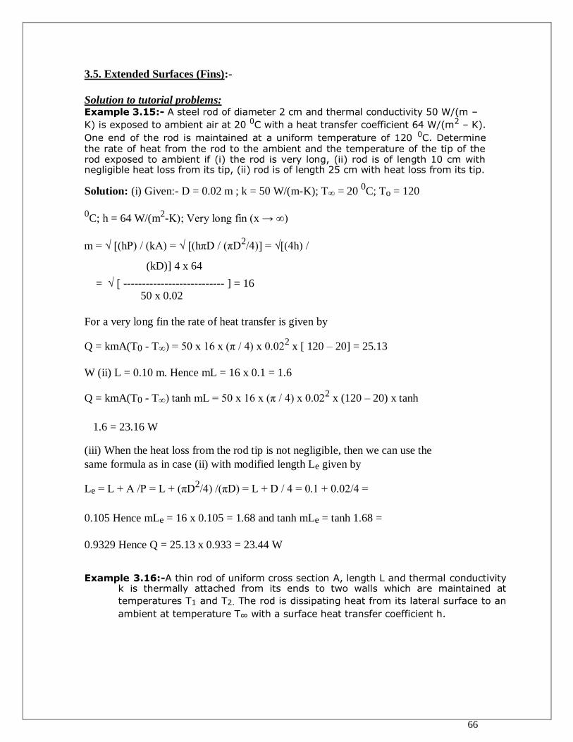
66

3.5. Extended Surfaces (Fins):-

Solution to tutorial problems:

Example 3.15:- A steel rod of diameter 2 cm and thermal conductivity 50 W/(m –

K) is exposed to ambient air at 20 0C with a heat transfer coefficient 64 W/(m2 – K).

One end of the rod is maintained at a uniform temperature of 120 0C. Determine the rate of heat from the rod to the ambient and the temperature of the tip of the rod exposed to ambient if (i) the rod is very long, (ii) rod is of length 10 cm with negligible heat loss from its tip, (ii) rod is of length 25 cm with heat loss from its tip.

Solution: (i) Given:- D = 0.02 m ; k = 50 W/(m-K); T∞ = 20 0C; To = 120

0C; h = 64 W/(m

2-K); Very long fin (x → ∞)

m = √ [(hP) / (kA) = √ [(hπD / (πD2/4)] = √[(4h) /

(kD)] 4 x 64

= √ [ --------------------------- ] = 16 50 x 0.02

For a very long fin the rate of heat transfer is given by

Q = kmA(T0 - T∞) = 50 x 16 x (π / 4) x 0.022 x [ 120 – 20] = 25.13

W (ii) L = 0.10 m. Hence mL = 16 x 0.1 = 1.6

Q = kmA(T0 - T∞) tanh mL = 50 x 16 x (π / 4) x 0.022 x (120 – 20) x tanh

1.6 = 23.16 W

(iii) When the heat loss from the rod tip is not negligible, then we can use the

same formula as in case (ii) with modified length Le given by

Le = L + A /P = L + (πD2/4) /(πD) = L + D / 4 = 0.1 + 0.02/4 =

0.105 Hence mLe = 16 x 0.105 = 1.68 and tanh mLe = tanh 1.68 =

0.9329 Hence Q = 25.13 x 0.933 = 23.44 W

Example 3.16:-A thin rod of uniform cross section A, length L and thermal conductivity k is thermally attached from its ends to two walls which are maintained at

temperatures T1 and T2. The rod is dissipating heat from its lateral surface to an

ambient at temperature T∞ with a surface heat transfer coefficient h.

67

(a) Obtain an expression for the temperature distribution along the length of the rod

(b) Also obtain an expression for the heat dissipation from the rod to the ambient

Solution: The general solution for the one-dimensional steady-state temperature distribution

along the length of a rod dissipating heat by convection from its lateral surface is given by

θ(x) = C1 cosh mx + C2 sinh mx ………………………..(1)

___________

where θ(x) = T(x) - T∞ ; m = √ (hP) / (kA) : P = perimeter of the rod = π D and A = Area of cross section of the rod = π D2 / 4.

The boundary conditions are: (i) at x = 0, T = T1 or θ = T1

- T∞ = θo (say).

(ii) at x = L, T = T2 or θ = T2

- T∞ = θL (say).

Condition(i) in Eq. (1) gives

θo = C1.

Condition (ii) in Eq. (1) gives

θL = θ0 cosh mL + C2 sinh mL

(θL ─ θo cosh mL)

C2 = ------------------------ . sinh mL

Substituting for C1 and C2 in Eq. (1) we have

(θL ─ θo cosh mL)

θ(x) = θo cosh mx + ------------------------ sinh mx

sinh mL

θo cosh mx sinh mL + θL sinh mx ─ θo cosh mL sinh mx 0r θ(x) = -----------------------------------------------------------------------

- sinh mL

θL sinh mx + θo sinh m(L – x)

0r θ(x) = -------------------------------------- ……………………………………..(2) sinh mL

Expression for the rate of heat dissipation from the rod:

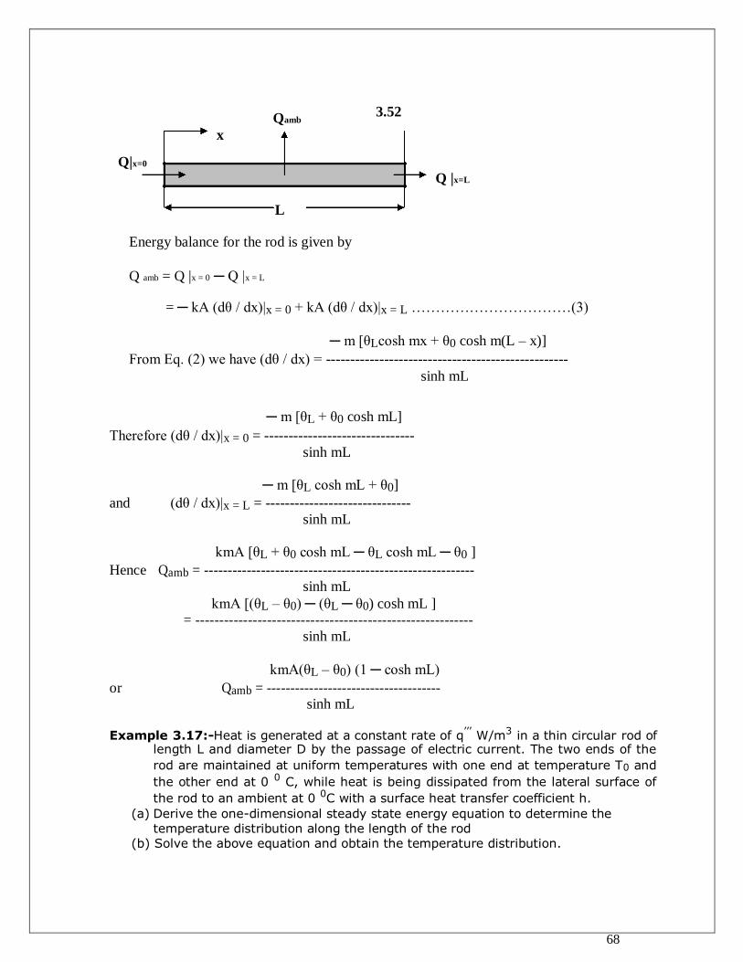
68

Qamb x

3.52

Q|x=0

Q |x=L

L

Energy balance for the rod is given by

Q amb = Q |x = 0 ─ Q |x = L

= ─ kA (dθ / dx)|x = 0 + kA (dθ / dx)|x = L ……………………………(3)

─ m [θLcosh mx + θ0 cosh m(L – x)] From Eq. (2) we have (dθ / dx) = --------------------------------------------------

sinh mL

─ m [θL + θ0 cosh mL]

Therefore (dθ / dx)|x = 0 = -------------------------------

sinh mL

─ m [θL cosh mL + θ0]

and (dθ / dx)|x = L = ------------------------------

sinh mL

kmA [θL + θ0 cosh mL ─ θL cosh mL ─ θ0 ]

Hence Qamb = ---------------------------------------------------------

sinh mL

kmA [(θL – θ0) ─ (θL ─ θ0) cosh mL ]

= ----------------------------------------------------------

sinh mL

kmA(θL – θ0) (1 ─ cosh mL)

or Qamb = -------------------------------------

sinh mL

Example 3.17:-Heat is generated at a constant rate of q’’’ W/m3 in a thin circular rod of length L and diameter D by the passage of electric current. The two ends of the

rod are maintained at uniform temperatures with one end at temperature T0 and

the other end at 0 0 C, while heat is being dissipated from the lateral surface of

the rod to an ambient at 0 0C with a surface heat transfer coefficient h. (a) Derive the one-dimensional steady state energy equation to determine the

temperature distribution along the length of the rod (b) Solve the above equation and obtain the temperature distribution.

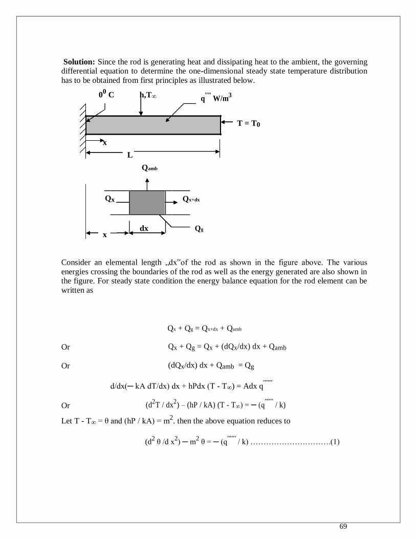
69

Solution: Since the rod is generating heat and dissipating heat to the ambient, the governing differential equation to determine the one-dimensional steady state temperature distribution

has to be obtained from first principles as illustrated below.

00 C h,T∞ q

’’’ W/m

3

x

T = T0

L

Qamb

Qx Qx+dx

Qg

x

dx

Consider an elemental length „dx‟of the rod as shown in the figure above. The various

energies crossing the boundaries of the rod as well as the energy generated are also shown in the figure. For steady state condition the energy balance equation for the rod element can be

written as

Qx + Qg = Qx+dx + Qamb

Or Qx + Qg = Qx + (dQx/dx) dx + Qamb

Or (dQx/dx) dx + Qamb = Qg

d/dx(─ kA dT/dx) dx + hPdx (T - T∞) = Adx q‟‟‟

Or (d2T / dx

2) – (hP / kA) (T - T∞) = ─ (q

‟‟‟ / k)

Let T - T∞ = θ and (hP / kA) = m2. then the above equation reduces to

(d2 θ /d x

2) ─ m

2 θ = ─ (q

‟‟‟ / k) ………………………….(1)

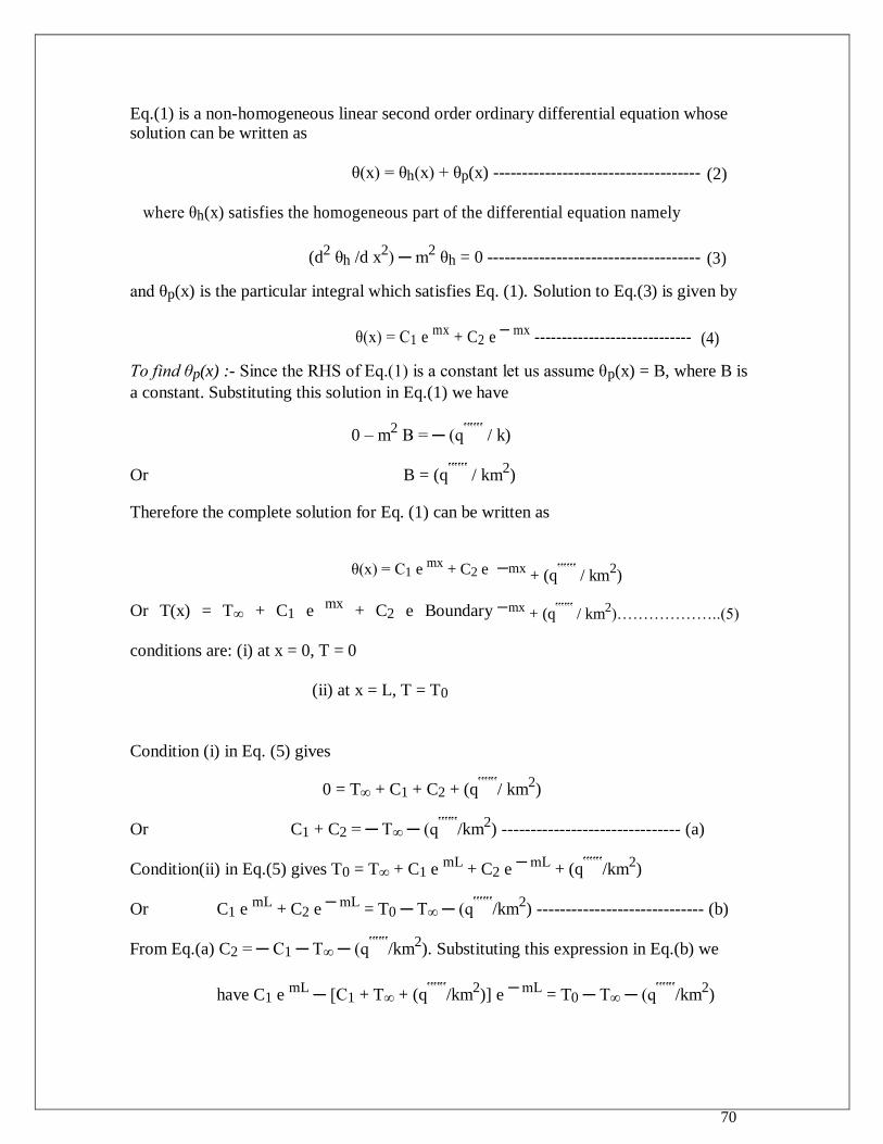
70

Eq.(1) is a non-homogeneous linear second order ordinary differential equation whose solution can be written as

θ(x) = θh(x) + θp(x) ------------------------------------ (2)

where θh(x) satisfies the homogeneous part of the differential equation namely

(d2 θh /d x

2) ─ m

2 θh = 0 ------------------------------------- (3)

and θp(x) is the particular integral which satisfies Eq. (1). Solution to Eq.(3) is given by

θ(x) = C1 e mx

+ C2 e ─ mx

----------------------------- (4)

To find θp(x) :- Since the RHS of Eq.(1) is a constant let us assume θp(x) = B, where B is

a constant. Substituting this solution in Eq.(1) we have

0 – m2 B = ─ (q

‟‟‟ / k)

Or B = (q‟‟‟

/ km2)

Therefore the complete solution for Eq. (1) can be written as

θ(x) = C1 e mx

+ C2 e

Or T(x) = T∞ + C1 e mx

+ C2 e Boundary

conditions are: (i) at x = 0, T = 0

(ii) at x = L, T = T0

─ mx + (q

‟‟‟ / km

2)

─ mx + (q

‟‟‟ / km

2)………………..(5)

Condition (i) in Eq. (5) gives

0 = T∞ + C1 + C2 + (q‟‟‟

/ km2)

Or C1 + C2 = ─ T∞ ─ (q‟‟‟

/km2) ------------------------------- (a)

Condition(ii) in Eq.(5) gives T0 = T∞ + C1 e mL

+ C2 e ─ mL

+ (q‟‟‟

/km2)

Or C1 e mL

+ C2 e ─ mL

= T0 ─ T∞ ─ (q‟‟‟

/km2) ----------------------------- (b)

From Eq.(a) C2 = ─ C1 ─ T∞ ─ (q‟‟‟

/km2). Substituting this expression in Eq.(b) we

have C1 e mL

─ [C1 + T∞ + (q‟‟‟

/km2)] e

─ mL = T0 ─ T∞ ─ (q

‟‟‟/km

2)

71

T0 ─ {T∞ + (q‟‟‟

/km2)}{1 ─ e

─ mL }

Solving for C1 we get C1 = --------------------------------------------------

{ e mL ─ e ─ mL }

T0 ─ {T∞ + (q‟‟‟

/km2)}{1 ─ e

─ mL }

C2 = ─{ T∞ + (q‟‟‟

/km2) }─ --------------------------------------------------

{ e mL

─ e ─ mL

}

─{ T∞ + (q‟‟‟

/km2) }{ e

mL ─ e

─ mL } ─ T0 + {T∞ + (q

‟‟‟/km

2)}{1 ─ e

─ mL }

C2 = ------------------------------------------------------------------------------------------------

{ e mL ─ e ─ mL }

{ T∞ + (q‟‟‟

/km2) }[ ─ e

mL + e

─ mL + 1 ─ e

─ mL] ─ T0

C2 = -----------------------------------------------------------------------------------------------

{ e mL

─ e ─ mL

}

{ T∞ + (q‟‟‟

/km2) }[ 1 ─ e

mL] ─ T0

C2 = ----------------------------------------------

{ e mL ─ e ─ mL }

Substituting the expressions for C1 and C2 in Eq. (5) and simplifying we get

T(x) = T∞ + (q‟‟‟

/km2) +

[T0 ─ {T∞ + (q‟‟‟

/km2)}{1 ─ e

─ mL }] e

mx

-------------------------------------------------{emL─e─mL}

+

[ { T∞ + (q‟‟‟

/km2) }[ 1 ─ e

mL] ─ T0] e

─ mx

----------------------------------------------------{emL─e─mL}

T(x) = T∞ + (q‟‟‟

/km2) +

T0(e mx

- e ─ mx

)

--------------------- +

{ e mL

─ e ─ mL

}

[ ─{T∞ + (q‟‟‟

/km2)}{ 1 ─ e

─ mL }] e

mx + { T∞ + (q

‟‟‟/km

2) }[ 1 ─ e

mL] e

─ mx]

----------------------------------------------------------------------------------------------

{ e mL ─ e ─ mL }

Example 3.18:- Two very long slender rods of the same diameter are given. One rod is of aluminum (k = 200 W/(m-K)). The thermal conductivity of the other

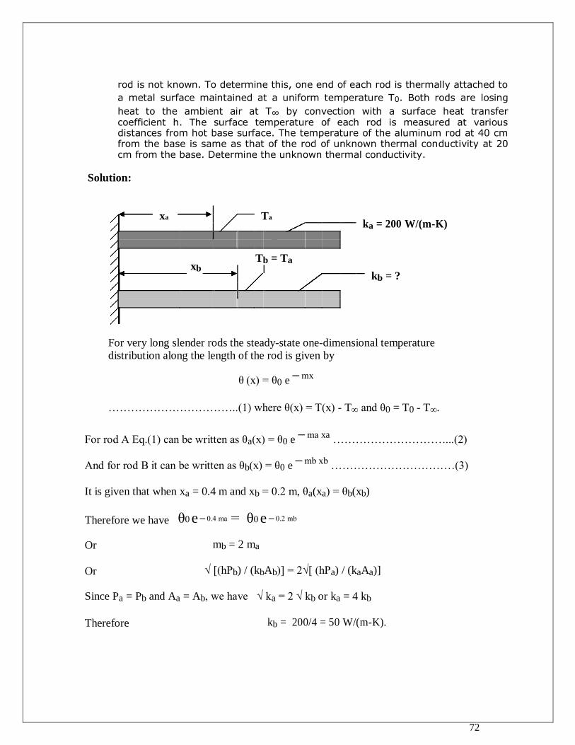
72

rod is not known. To determine this, one end of each rod is thermally attached to

a metal surface maintained at a uniform temperature T0. Both rods are losing

heat to the ambient air at T∞ by convection with a surface heat transfer coefficient h. The surface temperature of each rod is measured at various distances from hot base surface. The temperature of the aluminum rod at 40 cm from the base is same as that of the rod of unknown thermal conductivity at 20 cm from the base. Determine the unknown thermal conductivity.

Solution:

xa

Ta

ka = 200 W/(m-K)

xb

Tb = Ta

kb = ?

For very long slender rods the steady-state one-dimensional temperature distribution along the length of the rod is given by

θ (x) = θ0 e ─ mx

……………………………..(1) where θ(x) = T(x) - T∞ and θ0 = T0 - T∞.

For rod A Eq.(1) can be written as θa(x) = θ0 e ─ ma xa

…………………………...(2)

And for rod B it can be written as θb(x) = θ0 e ─ mb xb

……………………………(3)

It is given that when xa = 0.4 m and xb = 0.2 m, θa(xa) = θb(xb)

Therefore we have θ0 e ─ 0.4 ma = θ0 e ─ 0.2 mb

Or mb = 2 ma

Or √ [(hPb) / (kbAb)] = 2√[ (hPa) / (kaAa)]

Since Pa = Pb and Aa = Ab, we have √ ka = 2 √ kb or ka = 4 kb

Therefore kb = 200/4 = 50 W/(m-K).

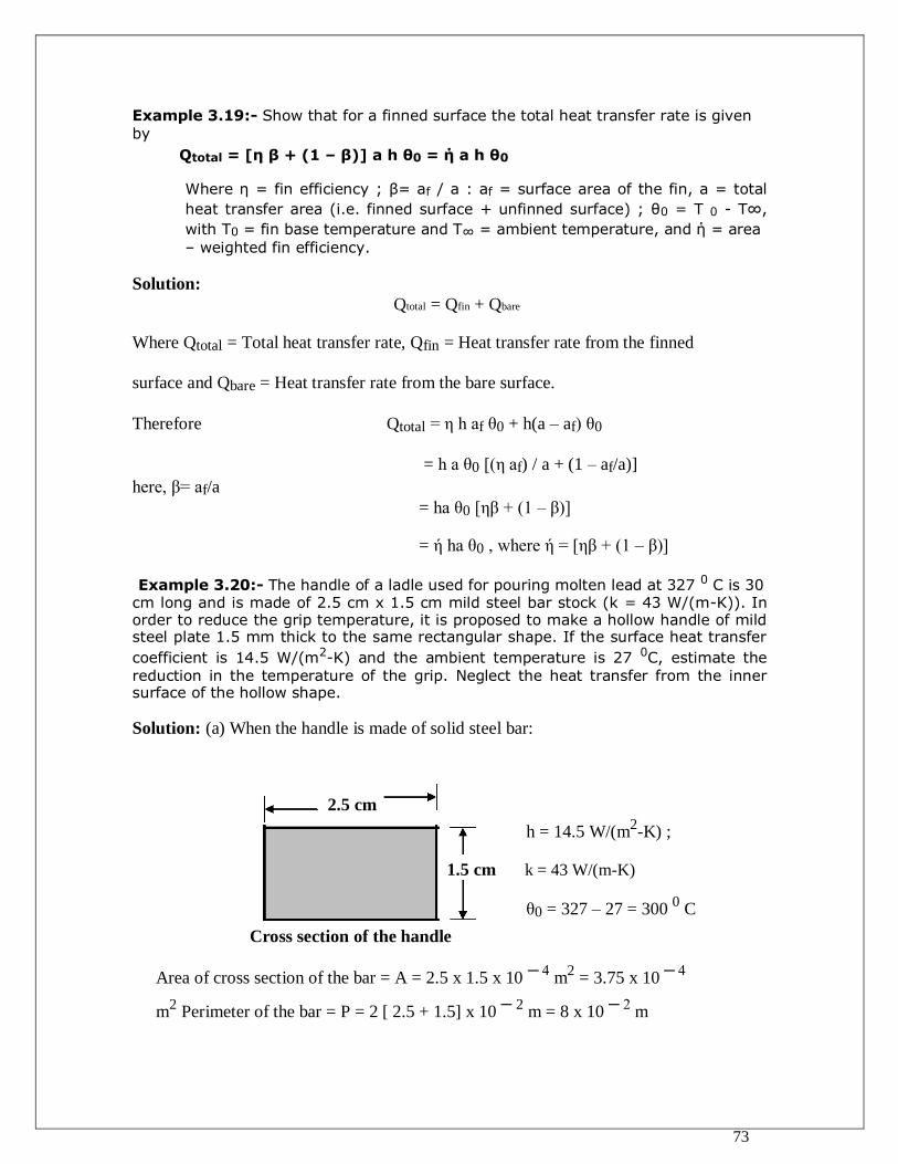
73

Example 3.19:- Show that for a finned surface the total heat transfer rate is given by

Qtotal = [η β + (1 – β)] a h θ0 = ή a h θ0

Where η = fin efficiency ; β= af / a : af = surface area of the fin, a = total

heat transfer area (i.e. finned surface + unfinned surface) ; θ0 = T 0 - T∞,

with T0 = fin base temperature and T∞ = ambient temperature, and ή = area

– weighted fin efficiency.

Solution: Qtotal = Qfin + Qbare

Where Qtotal = Total heat transfer rate, Qfin = Heat transfer rate from the finned

surface and Qbare = Heat transfer rate from the bare surface.

Therefore Qtotal = η h af θ0 + h(a – af) θ0

= h a θ0 [(η af) / a + (1 – af/a)]

here, β= af/a

= ha θ0 [ηβ + (1 – β)]

= ή ha θ0 , where ή = [ηβ + (1 – β)]

Example 3.20:- The handle of a ladle used for pouring molten lead at 327 0 C is 30

cm long and is made of 2.5 cm x 1.5 cm mild steel bar stock (k = 43 W/(m-K)). In order to reduce the grip temperature, it is proposed to make a hollow handle of mild steel plate 1.5 mm thick to the same rectangular shape. If the surface heat transfer

coefficient is 14.5 W/(m2-K) and the ambient temperature is 27 0C, estimate the

reduction in the temperature of the grip. Neglect the heat transfer from the inner surface of the hollow shape.

Solution: (a) When the handle is made of solid steel bar:

2.5 cm

h = 14.5 W/(m2-K) ;

1.5 cm k = 43 W/(m-K)

θ0 = 327 – 27 = 300 0 C

Cross section of the handle

Area of cross section of the bar = A = 2.5 x 1.5 x 10 ─ 4

m2 = 3.75 x 10

─ 4

m2 Perimeter of the bar = P = 2 [ 2.5 + 1.5] x 10

─ 2 m = 8 x 10

─ 2 m

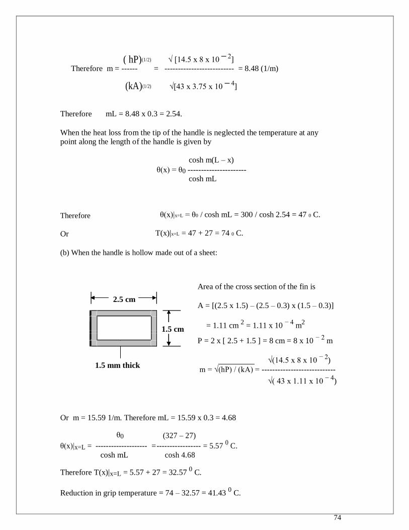
74

( hP)(1/2) √ [14.5 x 8 x 10 ─ 2

] Therefore m = ------ = -------------------------- = 8.48 (1/m)

(kA)(1/2) √[43 x 3.75 x 10 ─ 4

]

Therefore mL = 8.48 x 0.3 = 2.54.

When the heat loss from the tip of the handle is neglected the temperature at any point along the length of the handle is given by

cosh m(L – x)

θ(x) = θ0 ----------------------

cosh mL

Therefore

θ(x)|x=L = θ0 / cosh mL = 300 / cosh 2.54 = 47 0 C.

Or

T(x)|x=L = 47 + 27 = 74 0 C.

(b) When the handle is hollow made out of a sheet:

Area of the cross section of the fin is

2.5 cm

A = [(2.5 x 1.5) – (2.5 – 0.3) x (1.5 – 0.3)]

1.5 cm = 1.11 cm

2 = 1.11 x 10

− 4 m

2

P = 2 x [ 2.5 + 1.5 ] = 8 cm = 8 x 10

− 2 m

1.5 mm thick

_________ √(14.5 x 8 x 10 − 2

)

m = √(hP) / (kA) = ----------------------------

√( 43 x 1.11 x 10 − 4

)

Or m = 15.59 1/m. Therefore mL = 15.59 x 0.3 = 4.68

θ0 (327 – 27)

θ(x)|x=L = -------------------- = ----------------- = 5.57 0 C.

cosh mL cosh 4.68

Therefore T(x)|x=L = 5.57 + 27 = 32.57 0 C.

Reduction in grip temperature = 74 – 32.57 = 41.43 0 C.

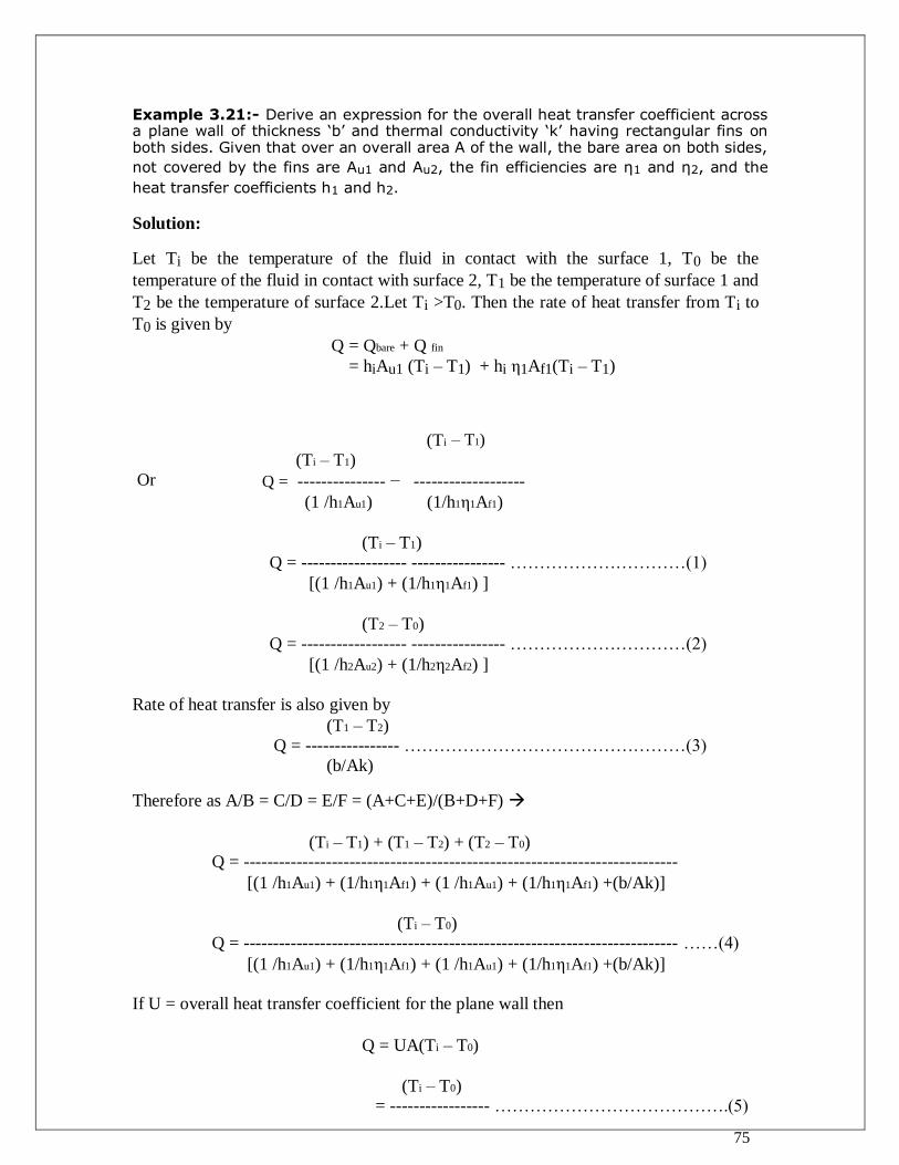
75

Example 3.21:- Derive an expression for the overall heat transfer coefficient across a plane wall of thickness ‘b’ and thermal conductivity ‘k’ having rectangular fins on both sides. Given that over an overall area A of the wall, the bare area on both sides,

not covered by the fins are Au1 and Au2, the fin efficiencies are η1 and η2, and the

heat transfer coefficients h1 and h2.

Solution:

Let Ti be the temperature of the fluid in contact with the surface 1, T0 be the

temperature of the fluid in contact with surface 2, T1 be the temperature of surface 1 and

T2 be the temperature of surface 2.Let Ti >T0. Then the rate of heat transfer from Ti to

T0 is given by Q = Qbare + Q fin

= hiAu1 (Ti – T1) + hi η1Af1(Ti – T1)

(Ti – T1)

(Ti

– T1)

Or Q =

--------------- − (1 /h1Au1)

-------------------

(1/h1η1Af1)

(Ti – T1) Q = ------------------ ---------------- …………………………(1)

[(1 /h1Au1) + (1/h1η1Af1) ]

(T2 – T0) Q = ------------------ ---------------- …………………………(2)

[(1 /h2Au2) + (1/h2η2Af2) ]

Rate of heat transfer is also given by (T1 – T2)

Q = ---------------- …………………………………………(3) (b/Ak)

Therefore as A/B = C/D = E/F = (A+C+E)/(B+D+F)

(Ti – T1) + (T1 – T2) + (T2 – T0) Q = --------------------------------------------------------------------------

[(1 /h1Au1) + (1/h1η1Af1) + (1 /h1Au1) + (1/h1η1Af1) +(b/Ak)]

(Ti – T0) Q = -------------------------------------------------------------------------- ……(4)

[(1 /h1Au1) + (1/h1η1Af1) + (1 /h1Au1) + (1/h1η1Af1) +(b/Ak)]

If U = overall heat transfer coefficient for the plane wall then

Q = UA(Ti – T0)

(Ti – T0) = ----------------- ………………………………….(5)

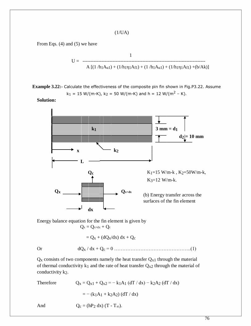
76

(1/UA)

From Eqs. (4) and (5) we have

1 U = ------------------------------------------------------------------------------

A [(1 /h1Au1) + (1/h1η1Af1) + (1 /h1Au1) + (1/h1η1Af1) +(b/Ak)]

Example 3.22:- Calculate the effectiveness of the composite pin fin shown in Fig.P3.22. Assume

k1 = 15 W/(m-K), k2 = 50 W/(m-K) and h = 12 W/(m2 – K).

Solution:

k1 3 mm = d1

d2 = 10 mm

x

k2

L

K1=15 W/m-k , K2=50W/m-k,

Qc

K3=12 W/m-k.

Qx

Qx+dx

(b) Energy transfer across the

surfaces of the fin element

dx

Energy balance equation for the fin element is given by

Qx = Qx+dx + Qc

= Qx + (dQx/dx) dx + Qc

Or dQx / dx + Qc = 0 ………………………………………..(1)

Qx consists of two components namely the heat transfer Qx1 through the material

of thermal conductivity k1 and the rate of heat transfer Qx2 through the material of

conductivity k2.

Therefore Qx = Qx1 + Qx2 = − k1A1 (dT / dx) − k2A2 (dT / dx)

= − (k1A1 + k2A2) (dT / dx)

And Qc = (hP2 dx) (T - T∞).

77

Substituting these expressions for Qx and Qc in equation (1) we get

hP2

(d2T / dx2) − ------------------- (T – T∞) = 0 (k1A1 + k2A2)

Or (d2θ / dx2) − m2 θ = 0 …………………………(2)

Where θ = T – T∞ and m = √ [ hP2 / (k1A1 + k2A2) ].

When the heat loss from the fin tip is negligible , the solution to equation (2) is given by

cosh [m(L – x)]

θ(x) = θ0 ---------------------- ………..(3) cosh mL

The rate of heat transfer from the fin base is given by

Qx|x=0 = − (k1A1 + k2A2) (dθ / dx)|x=0

− (k1A1 + k2A2) sinh [m(L – x)]x=0 (- m) θ0

= ---------------------------------------------------- cosh mL

= mθ0 (k1A1 + k2A2) tanh mL

Now η = Qx|x=0 / Qmax

mθ0 (k1A1 + k2A2) tanh mL

= ----------------------------------------

hP2L θ0

Noting that hP2 / (k1A1 + k2A2) = m2, the above expression for η simplifiers to

tanh mL η = ------------------------ ……………………(4)

mL

In the given problem A1 = (π / 4) x (0.003)2 = 7.1 x 10

− 6 m

2.

A2 = (π / 4) x [ (0.01)2 – (0.003)

2] = 7.15 x 10

− 5

P2 = π x 0.01 0.0314 m.

√ [ 12 x 0.0314] m = ----------------------------------------------------- = 10.12

√[(15 x 7.1 x 10 − 6

) + (50 x 7.15 x 10 − 5

)]

78

Therefore mL = 10.12 x 0.1 = 1.012

tanh (1.012) η = ------------------ = 0.757

1.012

Example 3.23:- Why is it necessary to derive a fresh differential equation for determining the one-dimensional steady state temperature distribution along the length of a fin?

Solution:- While deriving the conduction equation in differential form we will have

considered a differential volume element within the solid so that the heat transfer across

the boundary surfaces of the element is purely by conduction. But in the case of a fin the

lateral surface is exposed to an ambient so that the heat transfer across the lateral

surfaces is by convection. Therefore we have to derive the differential equation afresh

taking into account the heat transfer by convection across the lateral surfaces of the fin.

Solutions to Problems on Conduction in solids with variable thermal conductivity

Example 3.24:- A plane wall 4 cm thick has one of its surfaces in contact with a fluid at 130 0C with a surface heat transfer coefficient of 250 W/(m2 – K) and the other surface is in

contact with another fluid at 30 0C with a surface heat transfer coefficient of 500 W/(m2-K).

The thermal conductivity of the wall varies with temperature according to the law

k = 20 [ 1 + 0.001 T]

where T is the temperature. Determine the rate of heat transfer through the wall and the

surface temperatures of the wall.

Given:- L = 0.04 m; Ti = 130 0C; hi = 250 W/(m2-k); To = 30 0C; ho = 500

W/(m2-K); k = 20 [ 1 + 0.001 T].

To find:- (i) Qx (ii) T1 and T2

Solution:

Rci = Thermal resistance for convection at the surface at Ti = 1/(hiA) = 1 / (250 x

1) = 0.004 m2 – K /W

Rco = Thermal resistance for convection at the surface at To = 1/(hoA) = 1/(500 x 1)

79

Or Rco = 0.002 m2-K/W

Now Q = (Ti – T1) / Rci, where T1 = Surface temperature in contact with fluid at Ti.

Hence T1 = Ti – QRci = 130 – 0.004 Q ………………………………………….(1)

Similarly Q = (T2 – To) / Rco

Or T2 = To + QRco = 30 + 0.002Q ……………………………………………(2)

From equations (1) and (2) we have

T1 – T2 = 100 – 0.006Q ………………………………………………………….(3)

And Tm = ( T1 + T2) / 2 = 80 – 0.001Q ...……………………………………….(4)

Hence km = ko [ 1 + βTm] = 20 x [1 + 0.001x {80 – 0.001Q}]

= 21.6 – 2 x 10 − 5

Q

Hence thermal resistance offered by the wall = R = L/(Akm)

0.04 Or R = ---------------------------

[21.6 – 2 x 10 − 5

Q]

[T1 – T2] [100 – 0.006Q] [21.6 – 2 x 10 − 5

Q]

Q = --------------------- = --------------------------- x --------------------------

R 0.04

Cross multiplying we have

0.04Q = 2160 – 0.1316Q + 1.2 x 10 − 7

Q2

Or Q2 – 1.41 x 10

6 Q + 1.8 x 10

10 = 0.Hence Q = (1.41 x 10

6 ±1.39 x 10

6) / 2

For physically meaningful solution T1 should lie between Ti and To. This is possible

only If

Q = (1.41 x 10 6 − 1.39 x 10

6) / 2 = 10000 W.

Now T1 = Ti – QRci = 130 – 10000 x 0.004 = 90 0C

and T2 = T0 + Q Rco = 30 + 10000 x 0.002 = 50 0C.

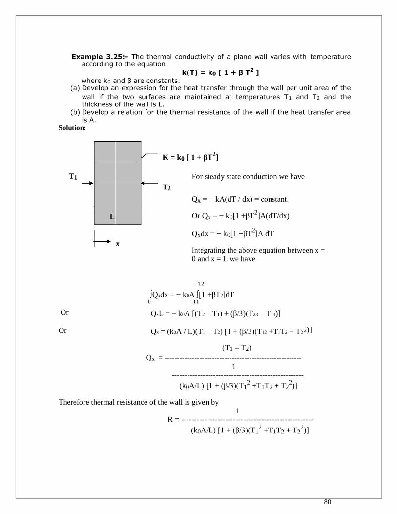
80

Example 3.25:- The thermal conductivity of a plane wall varies with temperature according to the equation

k(T) = k0 [ 1 + β T2 ]

where k0 and β are constants. (a) Develop an expression for the heat transfer through the wall per unit area of the

wall if the two surfaces are maintained at temperatures T1 and T2 and the thickness of the wall is L.

(b) Develop a relation for the thermal resistance of the wall if the heat transfer area is A.

Solution:

K = k0 [ 1 + βT

2]

T1 For steady state conduction we have

T2

Qx = − kA(dT / dx) = constant.

L Or Qx = − k0[1 +βT2]A(dT/dx)

Qxdx = − k0[1 +βT2]A dT

x

Integrating the above equation between x =

0 and x = L we have

T2

Or

Or

∫Qxdx = − k0A ∫[1 +βT2]dT

0 T1

QxL = − k0A [(T2 – T1) + (β/3)(T23 – T13)]

Qx = (k0A / L)(T1 – T2) [1 + (β/3)(T12 +T1T2 + T2

2)]

(T1 – T2)

Qx = -------------------------------------------------------

1

---------------------------------------------------

(k0A/L) [1 + (β/3)(T12 +T1T2 + T2

2)]

Therefore thermal resistance of the wall is given by

1

R = ---------------------------------------------------

(k0A/L) [1 + (β/3)(T12 +T1T2 + T2

2)]

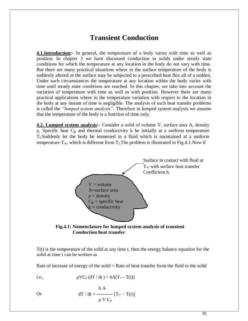
81

Transient Conduction

4.1.Introduction:- In general, the temperature of a body varies with time as well as

position. In chapter 3 we have discussed conduction in solids under steady state

conditions for which the temperature at any location in the body do not vary with time.

But there are many practical situations where in the surface temperature of the body is

suddenly altered or the surface may be subjected to a prescribed heat flux all of a sudden.

Under such circumstances the temperature at any location within the body varies with

time until steady state conditions are reached. In this chapter, we take into account the

variation of temperature with time as well as with position. However there are many

practical applications where in the temperature variation with respect to the location in

the body at any instant of time is negligible. The analysis of such heat transfer problems

is called the “lumped system analysis”. Therefore in lumped system analysis we assume

that the temperature of the body is a function of time only.

4.2. Lumped system analysis:- Consider a solid of volume V, surface area A, density

ρ, Specific heat Cp and thermal conductivity k be initially at a uniform temperature

Ti.Suddenly let the body be immersed in a fluid which is maintained at a uniform

temperature T∞, which is different from Ti.The problem is illustrated in Fig.4.1.Now if

Surface in contact with fluid at T∞ with surface heat transfer

Coefficient h

V = volume

A=surface area ρ = density

Cp = specific heat

k = conductivity

Fig.4.1: Nomenclature for lumped system analysis of transient Conduction heat transfer

T(t) is the temperature of the solid at any time t, then the energy balance equation for the solid at time t can be written as

Rate of increase of energy of the solid = Rate of heat transfer from the fluid to the solid

i.e.,

ρVCp (dT / dt ) = hA[T∞ - T(t)]

Or

h A

dT / dt = ---------- [T∞ − T(t)]

ρ V Cp

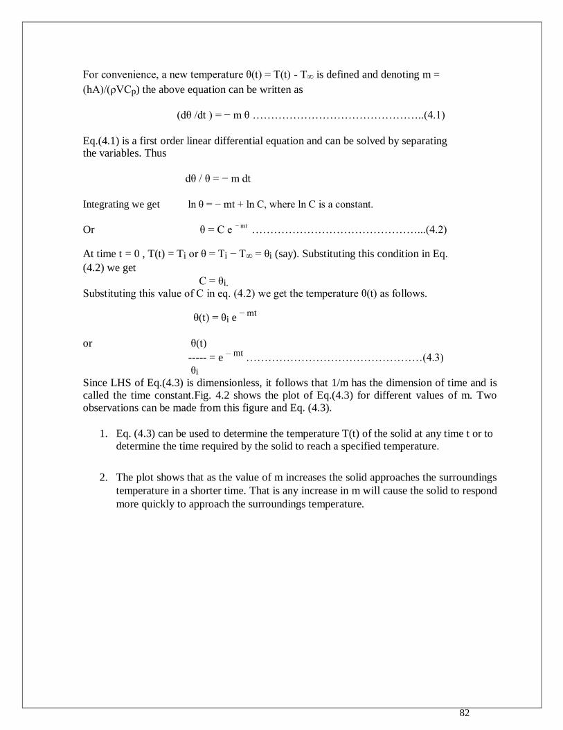
82

For convenience, a new temperature θ(t) = T(t) - T∞ is defined and denoting m =

(hA)/(ρVCp) the above equation can be written as

(dθ /dt ) = − m θ ………………………………………..(4.1)

Eq.(4.1) is a first order linear differential equation and can be solved by separating the variables. Thus

dθ / θ = − m dt

Integrating we get

ln θ = − mt + ln C, where ln C is a constant.

Or

θ = C e

− mt

………………………………………...(4.2)

At time t = 0 , T(t) = Ti or θ = Ti − T∞ = θi (say). Substituting this condition in Eq.

(4.2) we get

C = θi.

Substituting this value of C in eq. (4.2) we get the temperature θ(t) as follows.

θ(t) = θi e − mt

or θ(t)

----- = e – mt

…………………………………………(4.3)

θi Since LHS of Eq.(4.3) is dimensionless, it follows that 1/m has the dimension of time and is called the time constant.Fig. 4.2 shows the plot of Eq.(4.3) for different values of m. Two

observations can be made from this figure and Eq. (4.3).

1. Eq. (4.3) can be used to determine the temperature T(t) of the solid at any time t or to

determine the time required by the solid to reach a specified temperature.

2. The plot shows that as the value of m increases the solid approaches the surroundings

temperature in a shorter time. That is any increase in m will cause the solid to respond

more quickly to approach the surroundings temperature.

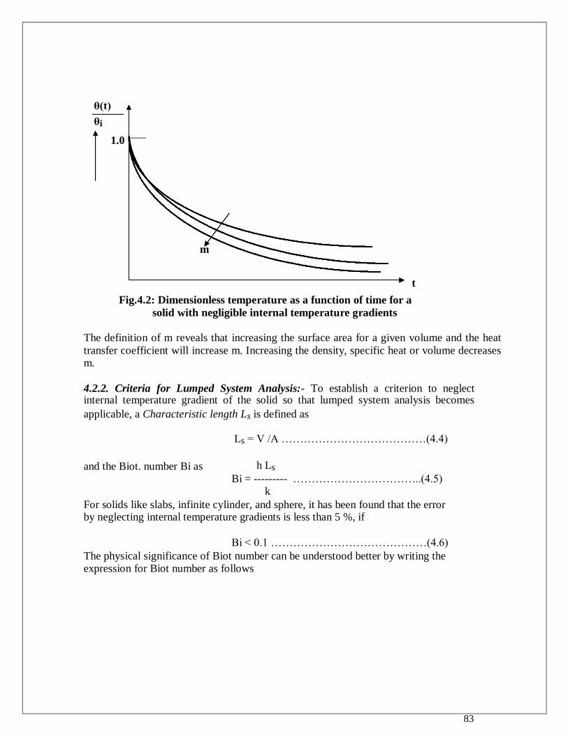
83

θ(t)

θi

1.0

m

t

Fig.4.2: Dimensionless temperature as a function of time for a

solid with negligible internal temperature gradients

The definition of m reveals that increasing the surface area for a given volume and the heat

transfer coefficient will increase m. Increasing the density, specific heat or volume decreases m.

4.2.2. Criteria for Lumped System Analysis:- To establish a criterion to neglect internal temperature gradient of the solid so that lumped system analysis becomes

applicable, a Characteristic length Ls is defined as

Ls = V /A …………………………………(4.4)

and the Biot. number Bi as h Ls

Bi = --------- ……………………………..(4.5)

k For solids like slabs, infinite cylinder, and sphere, it has been found that the error by neglecting internal temperature gradients is less than 5 %, if

Bi < 0.1 ……………………………………(4.6) The physical significance of Biot number can be understood better by writing the expression for Biot number as follows

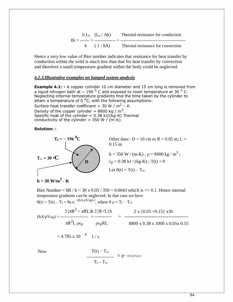
84

h Ls (Ls / Ak) Thermal resistance for conduction Bi = ------ = -------------- = -------------------------------------------

k ( 1 / hA) Thermal resistance for convection

Hence a very low value of Biot number indicates that resistance for heat transfer by conduction within the solid is much less than that for heat transfer by convection

and therefore a small temperature gradient within the body could be neglected.

4.2.3.Illustrative examples on lumped system analysis

Example 4.1: - A copper cylinder 10 cm diameter and 15 cm long is removed from

a liquid nitrogen bath at ─ 196 0 C and exposed to room temperature at 30 0 C. Neglecting internal temperature gradients find the time taken by the cylinder to attain a temperature of 0 0C, with the following assumptions:

Surface heat transfer coefficient = 30 W / m2 – K.

Density of the copper cylinder = 8800 kg / m3. Specific heat of the cylinder = 0.38 kJ/(kg-K) Thermal conductivity of the cylinder = 350 W / (m-K).

Solution: :

Ti = − 196 0C Other data:- D = 10 cm or R = 0.05 m; L =

0.15 m

k = 350 W / (m-K) ; ρ = 8800 kg / m3 ;

T∞ = 30 0C

D cp = 0.38 kJ / (kg-K) ; T(t) = 0

Let θ(t) = T(t) – T∞

h = 30 W/m2 - K

Biot Number = hR / k = 30 x 0.05 / 350 = 0.0043 which is << 0.1. Hence internal temperature gradients can be neglected. In that case we have

θ(t) = T(t) – Ti = θ0 e −(hA/ρVcp) t

, where θ 0 = Ti − T∞

2{πR2 + πRL)h 2{R+L}h 2 x {0.05 +0.15} x30

(hA/ρVcp) = ------------------- = ----------- = ------------------------------------------

πR2L ρcp ρcpRL 8800 x 0.38 x 1000 x 0.05x 0.15

= 4.785 x 10 − 4

1 / s

Now T(t) − T∞

= e − (hA/ρVcp) t

------------------

Ti – T∞

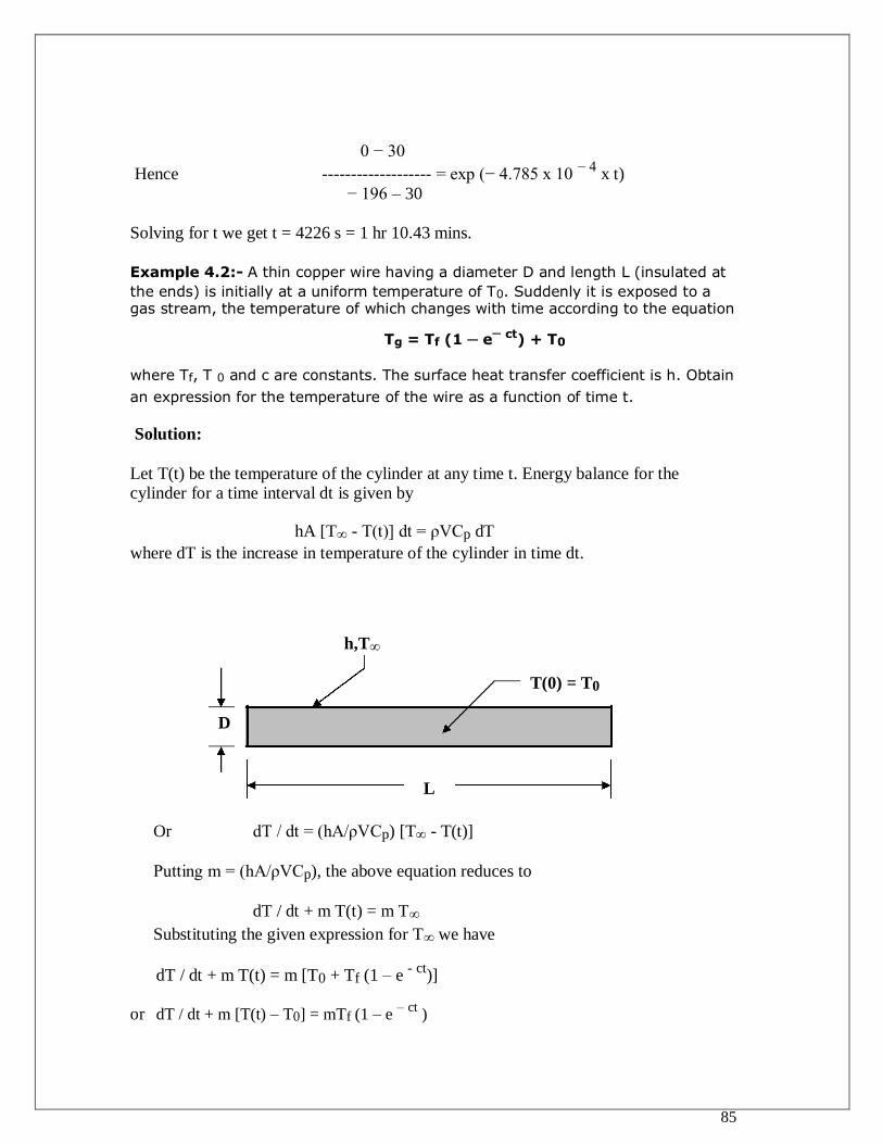
85

0 − 30

Hence ------------------- = exp (− 4.785 x 10 − 4

x t)

− 196 – 30

Solving for t we get t = 4226 s = 1 hr 10.43 mins.

Example 4.2:- A thin copper wire having a diameter D and length L (insulated at

the ends) is initially at a uniform temperature of T0. Suddenly it is exposed to a gas stream, the temperature of which changes with time according to the equation

Tg = Tf (1 ─ e─ ct) + T0

where Tf, T 0 and c are constants. The surface heat transfer coefficient is h. Obtain

an expression for the temperature of the wire as a function of time t.

Solution:

Let T(t) be the temperature of the cylinder at any time t. Energy balance for the cylinder for a time interval dt is given by

hA [T∞ - T(t)] dt = ρVCp dT where dT is the increase in temperature of the cylinder in time dt.

h,T∞

T(0) = T0

D

L

Or dT / dt = (hA/ρVCp) [T∞ - T(t)]

Putting m = (hA/ρVCp), the above equation reduces to

dT / dt + m T(t) = m T∞

Substituting the given expression for T∞ we have

dT / dt + m T(t) = m [T0 + Tf (1 – e - ct

)]

or dT / dt + m [T(t) – T0] = mTf (1 – e – ct

)

86

Let θ (t) = T(t) – T0. Then the above equation reduces to

dθ / dt + m θ (t) = mTf (1 – e – ct

)………………………………(1).

This equation is of the form dy / dx + Py = Q, which is solved by multiplying throughout by an integrating factor and then integrating. For equation (1) the integrating factor

is e ∫mdt

e mt

. therefore multiplying equation (1) by e mt

we get

e mt

(dθ / dt) + m e mt

θ (t) = mTf [ e mt

– e (m

– c)t

]

or d / dt (emt

θ) = mTf [ e mt

– e (m

– c)t

]

Integrating with respect to t we have

emt

θ(t) = mTf [ (emt

/ m ) − e(m

– c)t

/ (m – c) ] + C1

m

or θ(t) = Tf − ---------- Tf e − ct

+ C1e − mt

…………………(2)

( m – c )

When t = 0 , T(0) = T0 i.e., θ(0) = 0. Substituting this condition in equation (2) we get

m

or 0 = Tf − ---------- Tf + C1

( m – c )

Or C1 = [ c / (m – c)] Tf.

Substituting this expression for C1 in equation (2) we get the temperature of the

cylinder as

m c

θ(t) = Tf − ---------- Tf e − ct

+ ---------- Tf e − mt

( m – c ) (m – c)

Or T(t) – T0 = Tf [ 1 − m / (m – c) e − ct

+ c / (m – c) e − mt

]

Where m = hA / (ρVCp) = πDLh / {(πD2/4)LρCp}= (4h) /(ρDCp).

Example 4.3:- A solid sphere of radius R is initially at a uniform temperature T0. At a certain instant of time (t = 0), the sphere is suddenly exposed to the surroundings at a

temperature Tf and the surface heat transfer coefficient, ‘h’. In addition from the same

instant of time, heat is generated within the sphere at a uniform rate of q’’’ units per unit volume. Neglecting internal temperature gradients, derive an expression for the temperature of sphere as a function of time

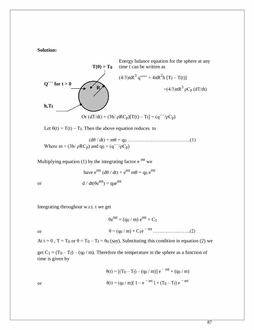
87

Solution:

T(0) = T0

Energy balance equation for the sphere at any time t can be written as

(4/3)πR3 q‟‟‟ + 4πR

2h [Tf – T(t)]

Q``` for t > 0

h,Tf

R

=(4/3)πR3 ρCp (dT/dt)

Or (dT/dt) + (3h/ ρRCp)[T(t) – Tf] = (q```/ρCp)

Let θ(t) = T(t) – Tf. Then the above equation reduces to

(dθ / dt) + mθ = q0 ………………………………..(1)

Where m = (3h/ ρRCp) and q0 = (q```/ρCp)

Multiplying equation (1) by the integrating factor e mt

we

have emt

(dθ / dt) + emt

mθ = q0 emt

or d / dt(θemt

) = q0emt

Integrating throughout w.r.t. t we get

θemt

= (q0 / m) emt

+ C1

or θ = (q0 / m) + C1e − mt

…………………...(2)

At t = 0 , T = T0 or θ = T0 – Tf = θ0 (say). Substituting this condition in equation (2) we

get C1 = (T0 – Tf) – (q0 / m). Therefore the temperature in the sphere as a function of

time is given by

θ(t) = [(T0 – Tf) – (q0 / m)] e − mt

+ (q0 / m)

or θ(t) = (q0 / m)[ 1 – e − mt

] + (T0 – Tf) e − mt

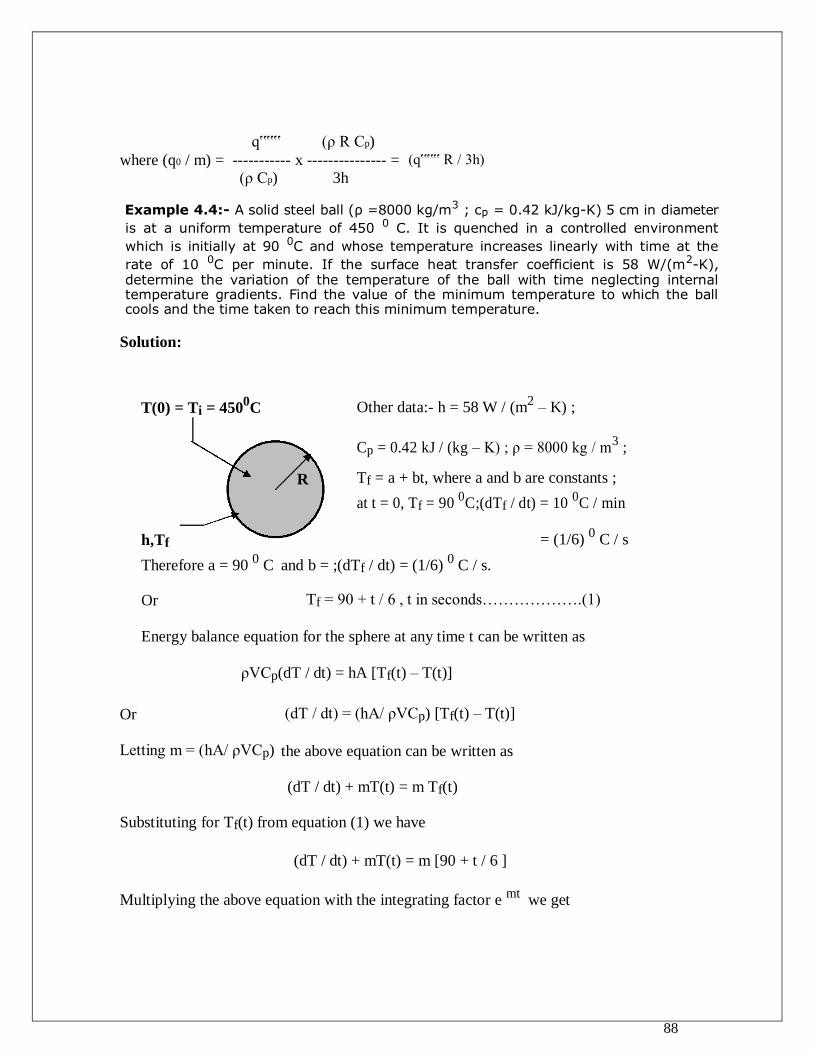
88

q‟‟‟ (ρ R Cp) where (q0 / m) = ----------- x --------------- =

(ρ Cp) 3h

(q‟‟‟ R / 3h)

Example 4.4:- A solid steel ball (ρ =8000 kg/m3 ; cp = 0.42 kJ/kg-K) 5 cm in diameter

is at a uniform temperature of 450 0 C. It is quenched in a controlled environment

which is initially at 90 0C and whose temperature increases linearly with time at the

rate of 10 0C per minute. If the surface heat transfer coefficient is 58 W/(m2-K), determine the variation of the temperature of the ball with time neglecting internal temperature gradients. Find the value of the minimum temperature to which the ball cools and the time taken to reach this minimum temperature.

Solution:

T(0) = Ti = 4500C Other data:- h = 58 W / (m

2 – K) ;

R

Cp = 0.42 kJ / (kg – K) ; ρ = 8000 kg / m3 ;

Tf = a + bt, where a and b are constants ;

at t = 0, Tf = 90 0C;(dTf / dt) = 10

0C / min

h,Tf

= (1/6) 0 C / s

Therefore a = 90 0 C and b = ;(dTf / dt) = (1/6)

0 C / s.

Or Tf = 90 + t / 6 , t in seconds……………….(1)

Energy balance equation for the sphere at any time t can be written as

ρVCp(dT / dt) = hA [Tf(t) – T(t)]

Or (dT / dt) = (hA/ ρVCp) [Tf(t) – T(t)]

Letting m = (hA/ ρVCp) the above equation can be written as

(dT / dt) + mT(t) = m Tf(t)

Substituting for Tf(t) from equation (1) we have

(dT / dt) + mT(t) = m [90 + t / 6 ]

Multiplying the above equation with the integrating factor e mt

we get

89

e mt

(dT / dt) + mT(t) emt

= m [90 + t / 6 ] e mt

or d / dt (T e mt

) = m [90 + t / 6 ] e mt

Integrating throughout w.r.t t we have

(T e mt

) = m ∫[90 + t / 6 ] e mt

dt + C1

Or T(t) = m e − mt

∫[90 + t / 6 ] e mt

dt + C1 e − mt

= m e − mt

[(90e mt

/m) + (temt

/6m) − (e mt

/6m2)] + C1 e

− mt

Or T(t) = [ 90 + (t / 6 ) − (1/6m)] + C1 e − mt

……………………..(2)

When t = 0 , T(t) = Ti. Substituting this condition in the above equation and solving

for C1 we get

C1 = [Ti – 90 + 1 / 6m]

Therefore the temperature of sphere as a function of time is given by

T(t) = [ 90 + (t / 6 ) − (1/6m)] + [Ti – 90 + 1 / 6m] e − mt

………….(3)

For T(t) to be extremum (dT / dt) = 0.

Therefore we have (dT / dt) = 1/6 + [Ti – 90 + 1 / 6m] e − mt

(− m) = 0

Substituting Ti = 450 0 C and simplifying we get

(360 m + 1/6) e − mt

= 1/6

Or e mt

= (2160 m + 1) -----------(4)

4πR2h 3 x 58

Now m = (hA / ρVCp) = -------------------- = (3h/ ρCpR) = -------------------------------------

[(4/3)πR3 ρCp] ( 8000 x 0.025 x 0.42 x 10

3)

= 2.07 x 10 − 3

.-------- (5)

Using (4) & (5) in (3),

T(t)= 90+ (t/6)- (1/(6x2.07x10-3

)) + [ 240-90+(1/(6x2.07x10-3

))] x exp{-2.07x10− 3

t}

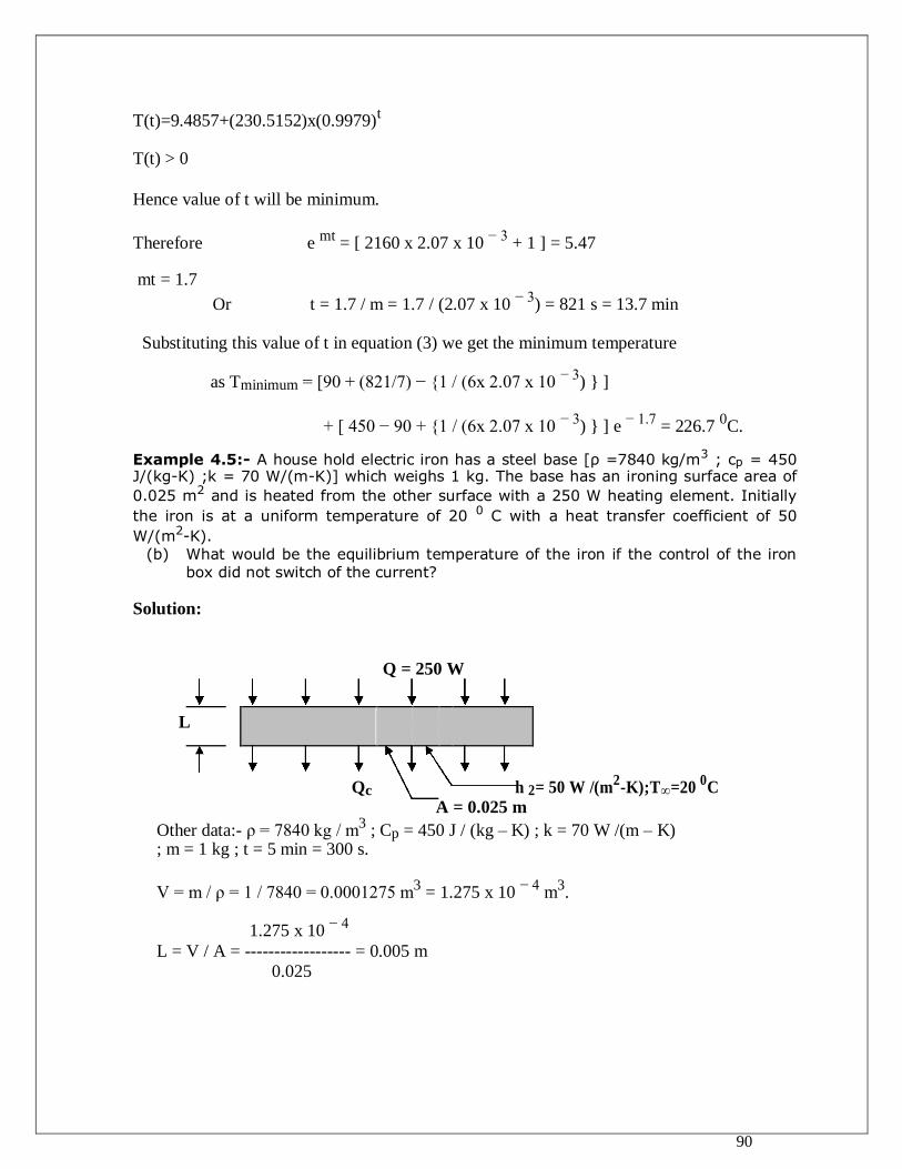
90

T(t)=9.4857+(230.5152)x(0.9979)t

T(t) > 0

Hence value of t will be minimum.

Therefore e mt

= [ 2160 x 2.07 x 10 − 3

+ 1 ] = 5.47

mt = 1.7

Or t = 1.7 / m = 1.7 / (2.07 x 10 − 3

) = 821 s = 13.7 min

Substituting this value of t in equation (3) we get the minimum temperature

as Tminimum = [90 + (821/7) − {1 / (6x 2.07 x 10 − 3

) } ]

+ [ 450 − 90 + {1 / (6x 2.07 x 10 − 3

) } ] e − 1.7

= 226.7 0C.

Example 4.5:- A house hold electric iron has a steel base [ρ =7840 kg/m3 ; cp = 450 J/(kg-K) ;k = 70 W/(m-K)] which weighs 1 kg. The base has an ironing surface area of

0.025 m2 and is heated from the other surface with a 250 W heating element. Initially

the iron is at a uniform temperature of 20 0 C with a heat transfer coefficient of 50

W/(m2-K). (b) What would be the equilibrium temperature of the iron if the control of the iron

box did not switch of the current?

Solution:

Q = 250 W

L

Qc h 2= 50 W /(m2-K);T∞=20

0C

A = 0.025 m

Other data:- ρ = 7840 kg / m3 ; Cp = 450 J / (kg – K) ; k = 70 W /(m – K)

; m = 1 kg ; t = 5 min = 300 s.

V = m / ρ = 1 / 7840 = 0.0001275 m3 = 1.275 x 10

− 4 m

3.

1.275 x 10 − 4

L = V / A = ------------------ = 0.005 m 0.025

91

50 x 0.005 Bi = (hL / k) = -------------------- = 0.00364

70

Since Bi < 0.1, it can be assumed that temperature gradients within the plate are negligible.

Hence the temperature of the plate depends only on time till steady state condition is reached.

Energy balance at any time t for the plate can be written as

Q − Qc = ρVCp (dT/dt)

Or Q – hA(T - T∞) = ρVCp (dT/dt)

Or (dT/dt) + m(T - T∞) = (Q / ρVCp) ……………………………..(1)

Where m = (hA / ρVCp). Letting θ = T - T∞, equation (1) can be written as

(dθ / dt) + m θ = (Q / ρVCp)

Multiplying the above equation by the integrating factor e mt

,( e∫mdt

=emt

) we get

(dθ / dt) e mt

+ m θe mt

= (Q / ρVCp) emt

Or d/dt (θe mt

) = (Q / ρVCp) emt

Or (θe mt

) = (Q / ρVCp) emt

(1/m) + C1

Or θ = (Q / ρVCpm) + C1e − mt

……………………………….(2)

When t = 0, T = Ti or θ = Ti - T∞ = 20 – 20 = 0 0 C.

Substituting this condition in equation (2) we get

0 = (Q / ρVCpm) + C1 or C1 = − (Q / ρVCpm)

Therefore the temperature in the plate as a function of time is given by

θ = (Q / ρVCpm) [ 1 − e − mt

] But ρVCpm = hA. Therefore

92

θ = (Q / hA) [ 1 − e − mt

] …………………………………..(3)

250 50 x 0.025

= 2.8 x 10-3

Q / hA = ------------------- = 200 ; m = -------------------

50 x 0.025 1 x 450

Therefore θ = 200 [ 1 – e −0.028t

]

When t = 300 s, θ = T - T∞ = 200 x [ 1 − e − 0.028 x 300

] = 113.7

Or T = 113.7 + 20 = 133.7 0 C.

(b) When the control switch is not switched off and the iron is left in the ambient, steady

state condition will be attained as t tends to ∞ so that the heat transferred to the baseplate will be convected to the ambient. i.e.,

Q = Qc

Therefore 250 = 50 x 0.025 x [T – 20 ]

Or T = 220 0 C.

This answer can also be obtained by putting t = ∞ in equation (3) and solving for T.

4.3 One-dimensional Transient Conduction ( Use of Heissler’s Charts): There are many

situations where we cannot neglect internal temperature gradients in a solid while analyzing

transient conduction problems. Then we have to determine the temperature distribution

within the solid as a function of position and time and the analysis becomes more complex.

However the problem of one-dimensional transient conduction in solids without heat

generation can be solved readily using the method of separation of variables.The analysis is

illustrated for solids subjected to convective boundary conditions and the solutions were

presented in the form of transient – temperature charts by Heissler. These charts are now

familiarly known as “Heissler‟s charts”.

4.3.1.One-dimensional transient conduction in a slab:- Let us consider a slab of thickness

2L, which is initially at a uniform temperature Ti. Suudenly let the solid be exposed to an

environment which is maintained at a uniform temperature of T∞ with a surface heat transfer

coefficient of h for time t > 0.Fig.4.3 shows the geometry , the coordinates and the boundary conditions for the problem. Because of symmetry in the problem with respect to the centre of the slab the „x‟ coordinate is measured from the centre line of the slab as shown in the figure.

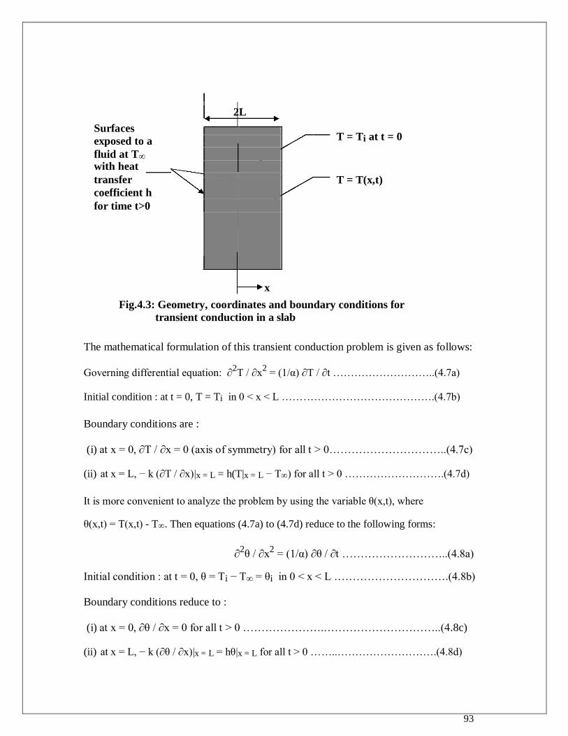
93

2L

Surfaces

T = Ti at t = 0

exposed to a

fluid at T∞

with heat

transfer

T = T(x,t)

coefficient h

for time t>0

x

Fig.4.3: Geometry, coordinates and boundary conditions for

transient conduction in a slab

The mathematical formulation of this transient conduction problem is given as follows:

Governing differential equation: ∂2T / ∂x

2 = (1/α) ∂T / ∂t ………………………..(4.7a)

Initial condition : at t = 0, T = Ti in 0 < x < L …………………………………….(4.7b)

Boundary conditions are :

(i) at x = 0, ∂T / ∂x = 0 (axis of symmetry) for all t > 0…………………………..(4.7c)

(ii) at x = L, − k (∂T / ∂x)|x = L = h(T|x = L − T∞) for all t > 0 ……………………….(4.7d)

It is more convenient to analyze the problem by using the variable θ(x,t), where

θ(x,t) = T(x,t) - T∞. Then equations (4.7a) to (4.7d) reduce to the following forms:

∂2θ / ∂x

2 = (1/α) ∂θ / ∂t ………………………..(4.8a)

Initial condition : at t = 0, θ = Ti − T∞ = θi in 0 < x < L ………………………….(4.8b)

Boundary conditions reduce to :

(i) at x = 0, ∂θ / ∂x = 0 for all t > 0 ………………….…………………………..(4.8c)

(ii) at x = L, − k (∂θ / ∂x)|x = L = hθ|x = L for all t > 0 ……..……………………….(4.8d)

94

Eq.(4.8a) can be solved by the method of separation of variables as shown below.

Let θ(x,t) = X(x) Y(t) ……………………………………………………………..(4.9)

Substituting this in Eq. (4.8a) we get

Y (d2X / dx

2) = (X/α) (dY / dt)

Or 1 1

--- (d2X / dx

2) = ------ (dY / dt) …………………….(4.10)

X (Yα)

LHS of Eq. (4.10) is a function of x only and the RHS of Eq. (4.10) is a function of t

only.They can be equal only to a constant say − λ2.(The reason to choose the negative

sign is to get a physically meaningful solution as explained later in this section).Hence we have two equations namely

(1 / X) (d2X / dx

2) = − λ

2 and [1/(Yα)] ((dY / dt) = − λ

2

Or (d2X / dx

2) + λ

2X = 0 ………………………………………………….(4.11)

and (dY/dt) = −αλ2 Y ………………………………………………………(4.12)

Solution to Eq. (4.11) is X(x) = C1 cos (λx) + C2 sin (λx) …………………….(4.13)

and solution to Eq. (4.12) is Y(t) = D exp (− αλ2t) ………………………..(4.14)

with C1, C2 and D as constants of integration. Substituting these solutions in Eq.(4.9)

we have

θ(x,t) = D exp (− αλ2t) [C1 cos (λx) + C2 sin (λx)]

or θ(x,t) = exp (− αλ2t) [A1 cos (λx) + A2 sin (λx)]………..(4.15)

Eq.(4.15) is the general solution involving the constants A1, A2 and λ which can be

determined using the two boundary conditions and the initial condition as

illustrated below.

Now from Eq. (4.15), ∂θ / ∂x = λ exp (− αλ2t) [ −A1 sin (λx) + A2 cos (λx)]

Substituting boundary condition (i) we have 0 = λ exp (− αλ2t) [0 + A2] for all

t. Hence A2 = 0. Therefore Eq. (4.15) reduce to

95

θ(x,t) = A1 exp (− αλ2t) cos (λx) ……………………….(4.16)

Now θ(L,t) = A1 exp (− αλ2t) cos (λL)

and ∂θ / ∂x = λ exp (− αλ2t) [ −A1 sin (λx) ]

Hence [∂θ / ∂x ] x = L = −λ A1 exp (− αλ2t) sin (λL)

Therefore boundary condition (ii) can be written as

k λ A1 exp (− αλ2t) sin (λL) = h A1 exp (− αλ

2t) cos (λL)

or tan (λL) = h / (kλ)

or λL tan (λL) = Bi ……………………………………………(4.17)

where Bi = hL / k. Equation (4.17) is called the “characteristic equation” and has infinite number of roots

namely λ1, λ2, λ3, .......Corresponding to each value of λ we have one solution and hence there are infinite number of solutions. Sum of all these solutions will also be a solution as the differential equation is linear. Therefore the solution θ(x,t) can be written as follows.

θ(x,t) = ∑ An exp (− αλn 2t) cos (λnx) …………………….(4.18)

To find An:- The constants An in Eq. (4.18) can be found using the orthogonal property

of trigonometric functions as shown below. Substituting the initial condition we have

θi = ∑ An cos (λnx)

Multiplying both sides of Eq.(4.18) by cos λmx and integrating w.r.t „x‟ between the limits 0 and L we have L L

∫ θi cos (λmx) dx = ∫ ∑ An cos (λmx) cos (λnx) dx 1 1

Using the orthogonal; property

∫ An cos (λmx) cos (λnx) dx = 0 for λn ≠ λm

The above equation reduce to

L L

∫ θi cos (λnx) dx = ∫ An cos 2(λnx) dx

0 0

L

θi 0 ∫cos (λnx) dx

Or An = ----L-------------------

∫ cos 2 (λnx)dx

0

96

It is very convenient to express Eq. (4.18) in dimension less form as follows:

θ(x,t)

----- = ∑ (An* exp (− λn

* 2 Fo) cos (λn* x / L) ………………………………(4.19)

θi

where An* = An / θi ; λn

* = λnL ; Fo = Fourier Number = α t / L

2 ;

4.3.2. Heissler’s Charts for transient conduction:- For values of Fo > 0.2 the above series

solution converges rapidly and the solution will be accurate within 5 % if only the first term in the series is used to determine the temperature. In that case the solution reduces to

θ(x,t)

----- = A1* exp (− λ1

* 2 Fo) cos (λ1* x /L) ……………………………………(4.20)

θi

From the above equation the dimensionless temperature at the centre of the slab (x =0) can be written as

θ(0,t)

----- = A1* exp (− λ1

* 2 Fo) ………………………………………………….(4.21)

θi

The values of A1* and λ1

* for different values of Bi are presented in the form of a table (See

Table 4.1). These values are evaluated using one term approximation of the series solution.It

can also be concluded from Eq.(4.20) at any time „t‟ the ratio θ(x,t) / θ(0,t) will be

independent of temperature and is given by

θ(x,t)

------ = cos (λ1* x /L) ……………………………………………………………(4.22)

θ(0,t)

Heissler has represented Eq. (4.21) and (4.22) in the form of charts and these charts are normally referred to as Heissler‟s charts. Eq. (4.21) is plotted as Fourier number Fo versus

dimensionless centre temperature θ(0,t) / θi using [Fig.4.4(b)]. reciprocal of Biot number1 / Bi as the parameter [Fig.4.4(a)], where as Eq. (4.22) is plotted as

θ(x,t) / θ(0,t) versus reciprocal of Biot number using the dimensionless distance x / L as the

parameter.In Fig.[4.4(a)], the curve for 1/Bi = 0 corresponds to the case h → ∞, or the outer surfaces of the slab are maintained at the ambient temperature T∞. For

large values of 1 / Bi, the Biot number is small, or the internal conductance is large in

comparison with the surface heat transfer coefficient. This in turn, implies that the

temperature distribution within the solid is sufficiently uniform and hence lumped system analysis becomes applicable.

Fig. (4.5) shows the dimensionless heat transferred Q / Q0 as a function of dimensionless time for different values of the Biot number for a slab of thickness 2L. Here Q represents the total amount of thermal energy which is lost by the slab up to any time t during

the transient conduction heat transfer. The quantity Q0, defined as

Q0 = ρ V Cp[Ti - T∞] …………………………..(4.23)

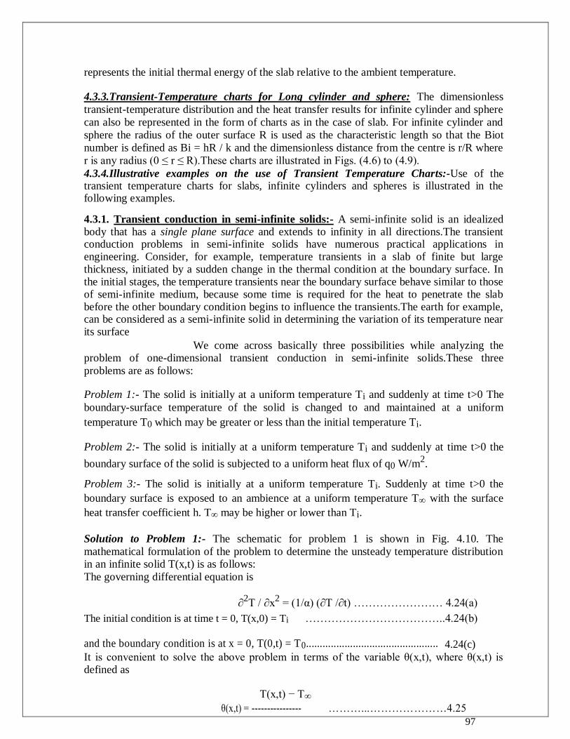
97

represents the initial thermal energy of the slab relative to the ambient temperature. 4.3.3.Transient-Temperature charts for Long cylinder and sphere: The dimensionless

transient-temperature distribution and the heat transfer results for infinite cylinder and sphere

can also be represented in the form of charts as in the case of slab. For infinite cylinder and

sphere the radius of the outer surface R is used as the characteristic length so that the Biot

number is defined as Bi = hR / k and the dimensionless distance from the centre is r/R where

r is any radius (0 ≤ r ≤ R).These charts are illustrated in Figs. (4.6) to (4.9). 4.3.4.Illustrative examples on the use of Transient Temperature Charts:-Use of the transient temperature charts for slabs, infinite cylinders and spheres is illustrated in the following examples.

4.3.1. Transient conduction in semi-infinite solids:- A semi-infinite solid is an idealized body that has a single plane surface and extends to infinity in all directions.The transient conduction problems in semi-infinite solids have numerous practical applications in engineering. Consider, for example, temperature transients in a slab of finite but large thickness, initiated by a sudden change in the thermal condition at the boundary surface. In the initial stages, the temperature transients near the boundary surface behave similar to those of semi-infinite medium, because some time is required for the heat to penetrate the slab before the other boundary condition begins to influence the transients.The earth for example, can be considered as a semi-infinite solid in determining the variation of its temperature near its surface

We come across basically three possibilities while analyzing the problem of one-dimensional transient conduction in semi-infinite solids.These three

problems are as follows:

Problem 1:- The solid is initially at a uniform temperature Ti and suddenly at time t>0 The

boundary-surface temperature of the solid is changed to and maintained at a uniform

temperature T0 which may be greater or less than the initial temperature Ti.

Problem 2:- The solid is initially at a uniform temperature Ti and suddenly at time t>0 the

boundary surface of the solid is subjected to a uniform heat flux of q0 W/m2.

Problem 3:- The solid is initially at a uniform temperature Ti. Suddenly at time t>0 the

boundary surface is exposed to an ambience at a uniform temperature T∞ with the surface

heat transfer coefficient h. T∞ may be higher or lower than Ti.

Solution to Problem 1:- The schematic for problem 1 is shown in Fig. 4.10. The

mathematical formulation of the problem to determine the unsteady temperature distribution in an infinite solid T(x,t) is as follows:

The governing differential equation is

∂2T / ∂x

2 = (1/α) (∂T /∂t) …………………… 4.24(a)

The initial condition is at time t = 0, T(x,0) = Ti ………………………………..4.24(b)

and the boundary condition is at x = 0, T(0,t) = T0................................................ 4.24(c)

It is convenient to solve the above problem in terms of the variable θ(x,t), where θ(x,t) is defined as

T(x,t) − T∞ θ(x,t) = ---------------- ………...…………………4.25

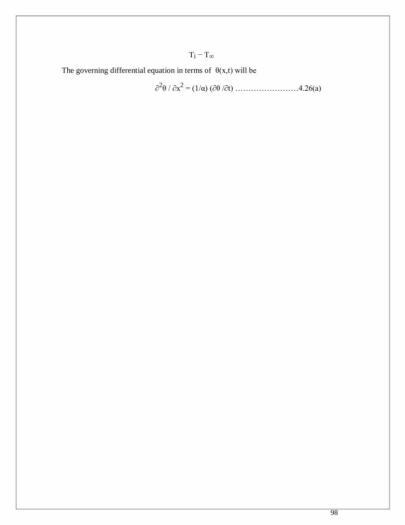
98

Ti − T∞

The governing differential equation in terms of θ(x,t) will be

∂2θ / ∂x

2 = (1/α) (∂θ /∂t) ……………………4.26(a)

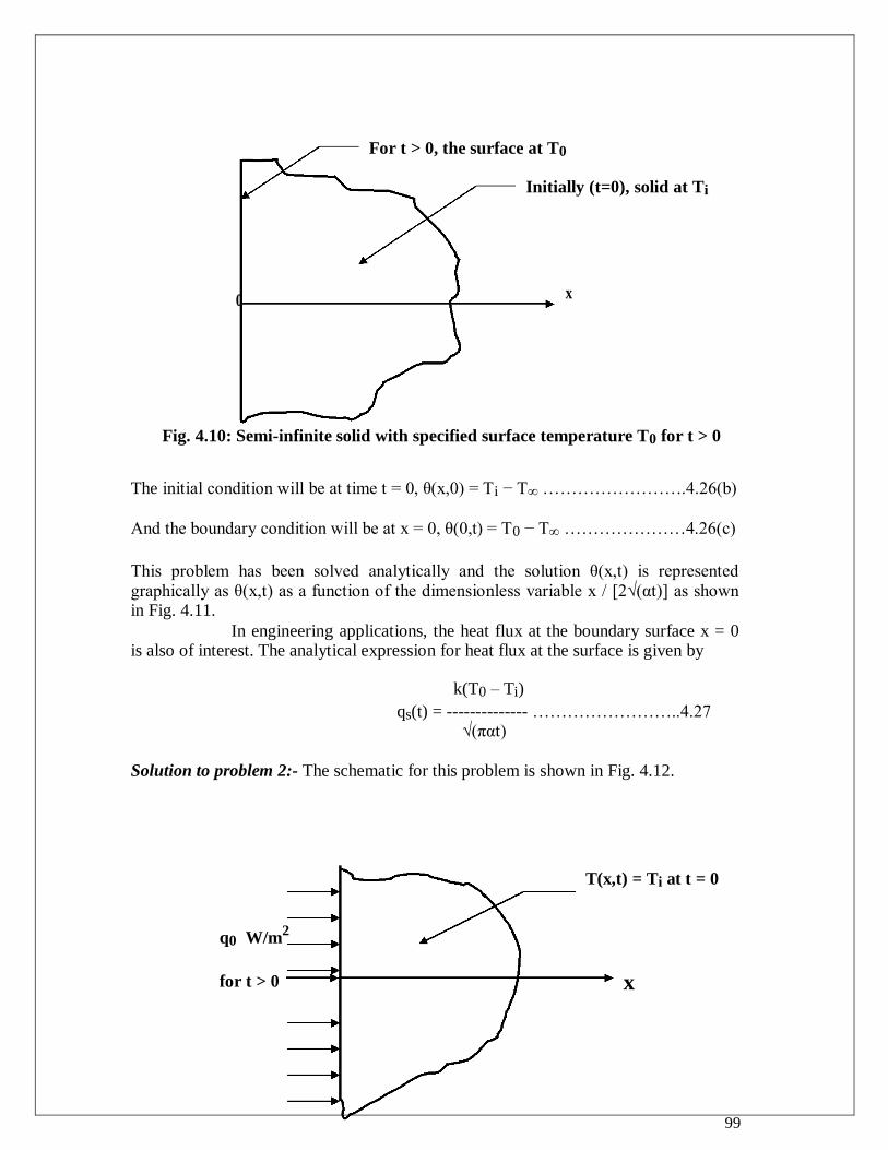
99

For t > 0, the surface at T0

Initially (t=0), solid at Ti

0 x

Fig. 4.10: Semi-infinite solid with specified surface temperature T0 for t > 0

The initial condition will be at time t = 0, θ(x,0) = Ti − T∞ …………………….4.26(b)

And the boundary condition will be at x = 0, θ(0,t) = T0 − T∞ …………………4.26(c)

This problem has been solved analytically and the solution θ(x,t) is represented

graphically as θ(x,t) as a function of the dimensionless variable x / [2√(αt)] as shown in Fig. 4.11.

In engineering applications, the heat flux at the boundary surface x = 0 is also of interest. The analytical expression for heat flux at the surface is given by

k(T0 – Ti)

qs(t) = -------------- ……………………..4.27

√(παt)

Solution to problem 2:- The schematic for this problem is shown in Fig. 4.12.

T(x,t) = Ti at t = 0

q0 W/m2

for t > 0 x

100

Fig. 4.12: An infinite solid subjected to a constant heat flux at x = 0 for t > 0

Governing differential equation in terms of T(x,t) and the initial condition are same that for problem 1[i.e. equations 4.26(a) and 4.26(b)].

The boundary condition is : at x = 0, − k (∂θ / ∂x)|x = 0 = q0.

The temperature distribution within the solid T(x,t) is given by

2q0

T(x, t) = Ti + ------ (αt) ½

[ (1 / √π) exp (− ξ2) + ξ erf (ξ) − ξ ] …………………..(4.28 a)

k ___ 2 ξ

where ξ = x / (2√ αt ) and erf (ξ) = ------- ∫ exp (− y2) dy ……………………...(4.28b)

√π 0

Here erf (ξ) is called the “error function” of argument ξ and its values for different values of

ξ are tabulated.

Solution to Problem 3 :- The solid is initially at a uniform temperature Ti and suddenly for t

>0 the surface at x = 0 is brought in contact with a fluid at a uniform temperature T∞ with a

surface heat transfer coefficient h. For this problem the solution is represented in the form of a plot where the dimensionless temperature [1 − θ(x,t)] is plottedagainst dimensionless distance x / √(αt), using h√(αt) / k as the parameter. It can be noted that the case h → ∞ is

equivalent to the boundary surface ay x = 0 maintained at a constant temperature T∞.

101

4.3.2. Illustrative examples on Transient Conduction in Semi – Infinite solids

Example 4.9:-A thick stainless steel slab [α = 1.6 x 10 ─ 5 m2/s and k = 61 W/(m-K)]

is initially at a uniform temperature of 150 0 C. Its surface temperature is suddenly

lowered to 20 0 C. By treating this as a one-dimensional transient conduction problem in a semi-infinite medium, determine the temperature at a depth 2 cm from the surface and the heat flux 1 minute after the surface temperature is lowered

Solution:

Ti = 150 0 C ; T0 = T|x=0 = 20

0 C ; α = 1.6 x 10

− 5 m

2 / s ; k = 61 W/(m – K) ; x = 0.02 m ;

T = 1 min = 60 s

x 0.02

ξ = -------------- = --------------------------------- = 0.323

2 √ (αt) 2 x √ ( 1.6 x 10 − 5

x 60)

T(x,t) – T0 From chart, --------------------- = 0.35

Ti – T0

Therefore T(x,t) = T0 + 0.35 (Ti – T0) = 20 + 0.35 x (150 – 20) = 65.5 0 C.

k(T0 – Ti) ------------------------------61x(20-150

= − 435.5 W / m2

qs(t) = --------------------- =

√ (παt) √ (π x 1.6 x 10 − 5

x 60)

Example 4.10:- A semi-infinite slab of copper (α = 1.1 x 10 ─ 4 m 2/s and k = 380

W/(m-K) is initially at a uniform temperature of 10 0 C. Suddenly the surface at x = 0 is

raised to 100 0C. Calculate the heat flux at the surface 5 minutes after rising of the surface temperature . How long will it take for the temperature at a depth of 5 cm from

the surface to reach 90 0 C?

Solution:

Ti = 10 0 C ; T0 = 100

0 C ; k = 380 W / (m – K) ; α = 1.1 x 10

− 4 m

2 / s; t = 300 s ;

k(T0 – Ti) 380 x (100 – 10)

qs(t) = ------------------- = -------------------------------- = 11012 W / m2 = 11.012 kW/m

2

√ (παt) √ (π x 1.1 x 10 − 4

x 300)

T(x,t) – T0 90 – 100

θ(x,t) = ------------------ = --------------------- = 0.11 . From chart ξ = 0.1

Ti – T0 10 – 100

x x2

0.05 2

102

ξ = -------------- or t = ------------------- = ------------------------------

2√ (αt) 4 α ξ 2 4 x 1.1 x 10

− 4 x (0.1)

2

= 586 s = 9.46 min

Example 4.11:-A thick bronze [α = 0.86 x 10 ─ 5 m2/s and k = 26 W/(m-K)] is initially

at 250 0 C. Suddenly the surface is exposed to a coolant at 25 0 C. If the surface heat

transfer coefficient is 150 W/(m2-K), determine the temperature 5 cm from the surface 10 minutes after the exposure.

Solution:

Ti = 250 0 C; T∞ = 25

0 C; h = 150 W/(m

2 – K) ; k = 26 W /(m – K) ; α = 0.86 x 10

−5 m

2/s

t = 600 s ; x = 0.05 m ;

x 0.05

ξ = ---------------- = ------------------------------------ = 0.35

2 √(α t) 2 x √ ( 0.86 x 10 − 5

x 600)

____ __________________

h √(α t) 150 x √ [ 0.86 x 10 − 5

x 600]

-------------- = -------------------------------------- = 0.414

K 26

[T(x,t) – T∞]

Therefore from chart 1 − ------------------------ = 0.15

(Ti – T∞)

Solving for T(x,t) we have T(x,t) = T∞ + (1 – 0.15)(Ti – T∞)

= 25 + 0.85 x (250 – 25 ) = 216.25 0 C.

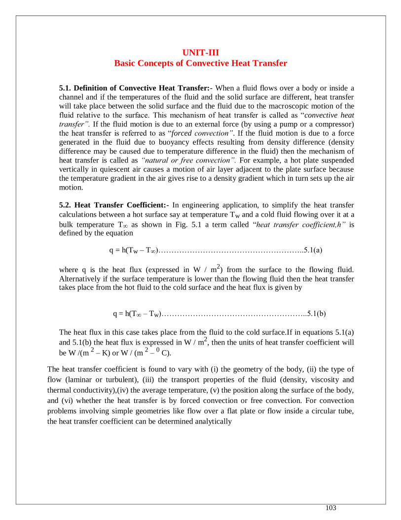
103

UNIT-III

Basic Concepts of Convective Heat Transfer

5.1. Definition of Convective Heat Transfer:- When a fluid flows over a body or inside a

channel and if the temperatures of the fluid and the solid surface are different, heat transfer

will take place between the solid surface and the fluid due to the macroscopic motion of the

fluid relative to the surface. This mechanism of heat transfer is called as “convective heat

transfer”. If the fluid motion is due to an external force (by using a pump or a compressor)

the heat transfer is referred to as “forced convection”. If the fluid motion is due to a force

generated in the fluid due to buoyancy effects resulting from density difference (density

difference may be caused due to temperature difference in the fluid) then the mechanism of

heat transfer is called as “natural or free convection”. For example, a hot plate suspended

vertically in quiescent air causes a motion of air layer adjacent to the plate surface because

the temperature gradient in the air gives rise to a density gradient which in turn sets up the air

motion.

5.2. Heat Transfer Coefficient:- In engineering application, to simplify the heat transfer

calculations between a hot surface say at temperature Tw and a cold fluid flowing over it at a

bulk temperature T∞ as shown in Fig. 5.1 a term called “heat transfer coefficient,h” is defined by the equation

q = h(Tw – T∞)………………………………………………..5.1(a)

where q is the heat flux (expressed in W / m2) from the surface to the flowing fluid.

Alternatively if the surface temperature is lower than the flowing fluid then the heat transfer takes place from the hot fluid to the cold surface and the heat flux is given by

q = h(T∞ – Tw)………………………………………………..5.1(b)

The heat flux in this case takes place from the fluid to the cold surface.If in equations 5.1(a)

and 5.1(b) the heat flux is expressed in W / m2, then the units of heat transfer coefficient will

be W /(m 2 – K) or W / (m

2 –

0 C).

The heat transfer coefficient is found to vary with (i) the geometry of the body, (ii) the type of

flow (laminar or turbulent), (iii) the transport properties of the fluid (density, viscosity and

thermal conductivity),(iv) the average temperature, (v) the position along the surface of the body,

and (vi) whether the heat transfer is by forced convection or free convection. For convection

problems involving simple geometries like flow over a flat plate or flow inside a circular tube,

the heat transfer coefficient can be determined analytically

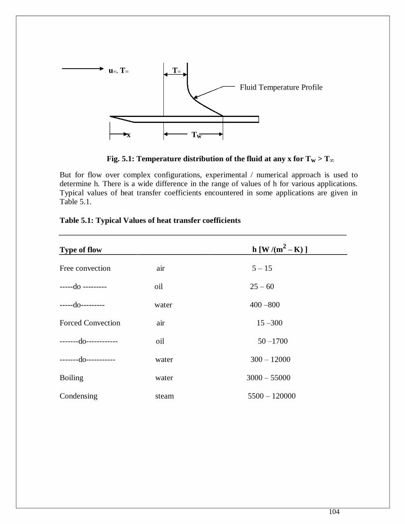
104

u∞, T∞ T∞

Fluid Temperature Profile

x Tw

Fig. 5.1: Temperature distribution of the fluid at any x for Tw > T∞

But for flow over complex configurations, experimental / numerical approach is used to determine h. There is a wide difference in the range of values of h for various applications.

Typical values of heat transfer coefficients encountered in some applications are given in Table 5.1.

Table 5.1: Typical Values of heat transfer coefficients

Type of flow h [W /(m2 – K) ]

Free convection air 5 – 15

-----do --------- oil 25 – 60

-----do--------- water 400 –800

Forced Convection air 15 –300

-------do------------ oil 50 –1700

-------do----------- water 300 – 12000

Boiling water 3000 – 55000

Condensing steam 5500 – 120000

105

5.3. Basic concepts for flow over a body:- When a fluid flows over a body, the velocity and

temperature distribution at the vicinity of the surface of the body strongly influence the heat

transfer by convection. By introducing the concept of boundary layers (velocity boundary

layer and thermal boundary layer) the analysis of convective heat transfer can be simplified.

5.3.1. Velocity Boundary Layer:- Consider the flow of a fluid over a flat plate as shown in Fig.

5.2. The fluid just before it approaches the leading edge of the plate has a velocity u∞ which is

parallel to the plate surface. As the fluid moves in x-direction along the plate,

y u∞

u(x, y)

u(x, y)

x xcr Turbulent Region

Laminar Region Transition

Fig. 5.2: Velocity boundary layer for flow over a flat plate

those fluid particles that makes contact with the plate surface will have the same velocity as that of the plate. Therefore if the plate is stationary, then the fluid layer sticking to the plate surface will have zero velocity.But far away from the plate (y = ∞) the fluid will have the velocity

u∞.Therefore starting from the plate surface (y = 0) there will be retardation of the fluid in x-

direction component of velocity u(x,y).This retardation effect is reduced as we move away from the plate surface.At distances sufficiently long from the plate(y = ∞) the retardation effect is

completely reduced: i.e. u → u∞ as y → ∞. This means that there is a region surrounding the

plate surface where the fluid velocity changes from zero at the surface to the velocity u∞ at the

outer edge of the region. This region is called the velocity boundary layer. The variation of the x-component of velocity u(x,y) with respect to y at a particular location along the plate is shown in Fig. 5.2.The distance measured normal to the surface from the plate surface to the point at which

the fluid attains 99% of u∞ is called “velocity boundary layer thickness” and denoted by δ(x)

Thus for flow over a flat plate, the flow field can be divided into two distinct regions, namely, (i) the boundary layer region in which the axial component of velocity u(x,y) varies rapidly with y

with the result the velocity gradient (∂u /∂y) and hence the shear stress are very large and (ii) the potential flow region which is outside the boundary layer region, where the velocity gradients and shear stresses are negligible.

106

The flow in the boundary layer, starting from the leading edge of the plate will be initially laminar in which the fluid particles move along a stream line in an orderly manner. In the laminar region the retardation effect is due to the viscosity of the fluid and therefore the shear stress can be evaluated using Newton‟s law of viscosity. The laminar

flow continues along the plate until a critical distance „xcr‟ is reached. After this the small

disturbances in the flow begin to grow and fluid fluctuations begin to develop. This characterizes the end of the laminar flow region and the beginning of transition from laminar to turbulent boundary layer. A dimensionless parameter called Reynolds number is used to characterize the flow as laminar or turbulent. For flow over a flat plate the Reynolds number is defined as

u∞ x

Rex = ---------- …………………………….5.2

ν

where u∞ = free-stream velocity of the fluid, x = distance from the leading edge of the plate and ν = kinematic viscosity of the fluid.

For flow over a flat plate it has been found that the transition from laminar

flow to turbulent flow takes place when the Reynolds number is ≈ 5 x 10 5.This number is called

as the critical Reynolds number Recr for flow over a flat plate. Therefore

u∞ xcr

Recr = -------------- = 5 x 10 5 ……………….5.3

ν The critical Reynolds number is strongly dependent on the surface roughness and the turbulence level of the free stream fluid. For example, with very large disturbances in the free

stream, the transition from laminar flow to turbulent flow may begin at Rex as low as 1 x 10 5

and for flows which are free from disturbances and if the plate surface is smooth transition

may not take place until a Reynolds number of 1 x 10 6 is reached. But it has been found that

for flow over a flat plate the boundary layer is always turbulent for Rex ≥ 4 x 10 6.In the

turbulent boundary layer next to the wall there is a very thin layer called “the viscous sub-layer”, where the flow retains its viscous flow character. Next to the viscous sub-layer is a region called “buffer layer” in which the effect of fluid viscosity is of the same order of magnitude as that of turbulence and the mean velocity rapidly increases with the distance from the plate surface. Next to the buffer layer is “the turbulent layer” in which there is large scale turbulence and the velocity changes relatively little with distance.

5.3.2. Drag coefficient and Drag force:- If the velocity distribution u(x,y) in the boundary layer at any „x‟ is known then the viscous shear stress at the wall can be determined using

Newton‟s law of viscosity. Thus if ηw(x) is the wall-shear stress at any location x then

107

ηw(x) = μ(∂u / ∂y)y = 0 ………………….5.4

where μ is the absolute viscosity of the fluid. The drag coefficient is dimensionless wall

shear stress. Therefore the local drag coefficient, Cx at any „x‟ is defined as

ηw(x)

Cx = ------------- ……………………….5.5

(1/2) ρu∞2

Substituting for ηw(x) in the above equation from Eq. 5.4 and simplifying we get

2ν (∂u / ∂y)y = 0

Cx = ---------------------- ……………….5.6

u∞2

Therefore if the velocity profile u(x,y) at any x is known then the local drag

coefficient Cx at that location can be determined from Eq. 5.6.The average value of Cx for a total length L of the plate can be determined from the equation

L

Cav = (1/L) ∫Cx dx ……………………5.7

0

Substituting for Cx from Eq. 5.5 we have

L

∫ ηw(x)dx

Cav = ------------------------

2

L (1/2) ρu∞

_

ηw

Or Cav = -------------------- ……………….5.8

(1/2) ρu∞2

_

Where ηw is the average wall-shear stress for total length L of the plate.

The total drag force experienced by the fluid due to the presence of the plate can be written as

_

FD = As ηw …………………………….5.9

Where As is the total area of contact between the fluid and the plate. If „W‟ is the

width of the plate then As = LW if the flow is taking place on one side of the plate and

As = 2LW if the flow is on both sides of the plate.

5.3.3. Thermal boundary layer:- Similar to the velocity boundary layer one can visualize the

development of a thermal boundary layer when a fluid flows over a flat

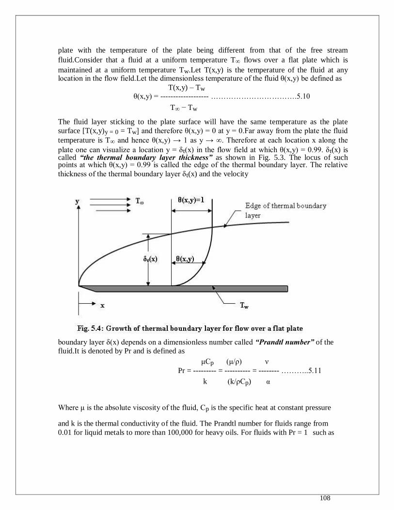
108

plate with the temperature of the plate being different from that of the free stream

fluid.Consider that a fluid at a uniform temperature T∞ flows over a flat plate which is

maintained at a uniform temperature Tw.Let T(x,y) is the temperature of the fluid at any location in the flow field.Let the dimensionless temperature of the fluid θ(x,y) be defined as

T(x,y) – Tw

θ(x,y) = ------------------- …………………………….5.10

T∞ − Tw

The fluid layer sticking to the plate surface will have the same temperature as the plate

surface [T(x,y)y = 0 = Tw] and therefore θ(x,y) = 0 at y = 0.Far away from the plate the fluid

temperature is T∞ and hence θ(x,y) → 1 as y → ∞. Therefore at each location x along the

plate one can visualize a location y = δt(x) in the flow field at which θ(x,y) = 0.99. δt(x) is called “the thermal boundary layer thickness” as shown in Fig. 5.3. The locus of such points at which θ(x,y) = 0.99 is called the edge of the thermal boundary layer. The relative

thickness of the thermal boundary layer δt(x) and the velocity

boundary layer δ(x) depends on a dimensionless number called “Prandtl number” of the

fluid.It is denoted by Pr and is defined as

μCp (μ/ρ) ν

Pr = --------- = ---------- = -------- ………..5.11

k (k/ρCp) α

Where μ is the absolute viscosity of the fluid, Cp is the specific heat at constant pressure

and k is the thermal conductivity of the fluid. The Prandtl number for fluids range from 0.01 for liquid metals to more than 100,000 for heavy oils. For fluids with Pr = 1 such as

109

gases δt(x) = δ(x), for fluids with Pr << 1such as liquid metals δt(x) >> δ(x) and for

fluids with Pr >> 1, like oils δt(x) << δ(x).

5.3.4. General expression for heat transfer coefficient:- Let us assume that Tw >

T∞. Then heat is transferred from the plate to the fluid flowing over the plate.Therefore at any „x‟ the heat flux is given by

q = − k (∂T /∂y)y=0 ………………………..5.12(a)

In terms of the local heat transfer coefficient hx, the heat flux can also be written as

q = hx (Tw − T∞) …………………………..5.12(b)

From equations 5.12(a) and 5.12(b) it follows that

− k (∂T /∂y)y=0

hx = ------------------ ………………………5.13

(Tw − T∞)

From equation 5.10 we have (∂T /∂y)y=0 = [T∞ − Tw] (∂θ /∂y)y=0. Substituting this

expression in Eq.5.13 and simplifying we get the general expression for hx as

hx = k (∂θ /∂y)y=0 ………………………….5.14

The same expression for hx could be obtained even when Tw < T∞. Equation 5.14 can

be used to determine the local heat transfer coefficient for flow over a flat plate if the

dimensionless temperature profile θ(x,y) is known.

Average heat transfer coefficient:- For a total length L of the plate the average heat transfer coefficient is given by

L

hav = (1 /L) ∫hxdx ………………………….5.15 0

Substituting for hx from Eq. 5.14 we get

L

hav = (1 /L) ∫ k (∂θ /∂y)y=0 dx ………………….5.15 0

Since (∂θ /∂y)y=0 at any x depends on whether the flow at that section is laminar

or turbulent the expression for hav can be written as

xcr L

hav = (1 /L) { ∫ k [(∂θ /∂y)y=0]laminar dx + ∫ k [(∂θ /∂y)y=0]turbulent dx }……5.16

110

Example 5.1:- Assuming the transition from laminar to turbulent flow takes place at a

Reynolds number of 5 x 10 5, determine the distance from the leading edge of a flat plate

at which transition occurs for the flow of each of the following fluids with a velocity of 2

crm/s at 40 0 C.(i) Air at atmospheric pressure;(ii)Hydrogen at atmospheric

pressure;(iii) water;(iv) Engine oil;(v) mercury. Comment on the type of flow for the 5 fluids if the total length of the plate is 1 m.

Solution: Data:- Recr = 5 x 10 5; u∞ = 2 m/s ; T∞ = 40

0 C

(i)Air at atmospheric pressure :- At 40 0 C, ν = 17 x 10

− 6 m

2/s.

u∞ xcr Recr ν 5 x 10 5 x 17 x 10

− 6

Recr = ----------- or xcr = -------------------- = ---------------------------- = 4.25 m.

ν u∞ 2

(ii) Hydrogen :- For hydrogen at 40 0 C, ν = 117.9 x 10

− 6 m

2/s.

5 x 10 5 x 117.9 x 10

− 6

Therefore xcr = ------------------------------- = 29.5 m

2

(iii) Water :- For water at 40 0 C, ν = 0.658 x 10

− 6 m

2/s.

5 x 10 5 x 0.658 x 10

− 6

Therefore xcr = ------------------------------- = 0.1645 m

2

(iv) Engine oil :- For engine oil at 40 0 C, ν = 0.24 x 10

− 3 m

2/s.

5 x 10 5 x 0.24 x 10

− 3

Therefore xcr = -------------------------------2

= 60 m

(v) Mercury :- For mercury at 40 0 C, ν = 0.107 x 10

− 6 m

2/s.

5 x 10 5 x 0.107 x 10

− 6

Therefore xcr = ------------------------------- = 0.027 m

2

111

Comments on the type of flow

Sl.No Type of fluid xcr xcr vs L Type of Flow

1 Air 4.25 xcr > L Flow is Laminar for entire length

2 Hydrogen 29.5 xcr>> L Flow is laminar for entire length

3 Water 0.1645 xcr < L Flow is partly Laminar & Partly Turbulent

4 Engine oil 60 xcr >> L Flow is laminar for entire length

5 Mercury 0.027 xcr << L Flow is turbulent for almost entire length

Example 5.2:- An approximate expression for the velocity profile u(x,y) for laminar

boundary layer flow along a flat plate is given by

u(x, y)/ u∞ =2[y / δ(x)] − 2[y / δ(x)] 3+ [y / δ(x)]

4

where δ(x) is the velocity boundary layer thickness given by the expression

δ(x) / x = 5.83 / (Rex)1/2

(a) Develop an expression for the local drag coefficient.

(b) Develop an expression for the average drag coefficient for a length L of the plate. (c) Determine the drag force acting on the plate 2 m x 2 m for flow of air with a

free stream velocity of 4 m /s and a temperature of 80 0C.

Solution:- (a) The velocity profile u(x,y) is given as

u(x, y) = u∞ {2[y / δ(x)] − 2[y / δ(x)] 3+ [y / δ(x)]

4 }

Therefore (∂u / ∂y)y=0 = 2u∞ / δ(x)

ηw(x) = μ (∂u / ∂y)y=0 = (2 μu∞) / δ(x)

(2 μu∞) Rex (2 μu∞) [(u∞x) / ν]1/2

= ----------------- = ------------------------ = 0.343 (μu∞) [u∞ /(x ν)]1/2

….(1 )

5.83 x 5.83 x

112

The local drag coefficient at any x is given by

ηw(x) 0.343 (μu∞) [u∞ /(x ν)]1/2

Cx = ----------------- = -------------------------------------------

(1/2) ρu∞2 (1/2) ρu∞

2

0.686 0.686

= ---------------------- = -----------------

{(u∞x) / ν}1/2

(Rex) ½

(b) The average drag coefficient is given by

L L

Cav = (1/L) ∫ Cx dx = (1/L) ∫ 0.686 (Rex) − ½

dx

0 0

{ 0.686 (u∞/ν) − ½

} L

= ----------------------- ∫ x − ½

dx

L 0

Or 2 x 0.686 1.372

Cav = --------------- = ------------------

(u∞L / ν) ½

(ReL) ½

(c) At 80 0 C for air ν = 20.76 x 10

− 6 m

2 / s ; ρ = 1.00 kg / m

3

u∞L 4 x 2

ReL = ----------------- = ------------------- = 3.793 x 10 5

ν 21.09 x 10 − 6

1.372 1.372

Average drag coefficient = Cav = ------------------- = ------------------------ = 2.228 x 10 − 3

ReL0.5

(3.793 x 10 5)0.5

Drag force assuming that the flow takes place on one side of the plate is given by

FD = ηw LW = (1/2)ρ u∞2 Cav LW for flow over one side of the plate

= (1/2) x 1.00 x 42 x 2.2228 x 10

− 3 x 2 x 2 =0.071 N

113

Example 5.3:- An approximate expression for temperature profile θ(x,y) in the thermal boundary layer region is given by

θ(x,y) = 2y / δt −[y / δt]2

where the thermal boundary layer thickness δt is given by 5.5

δt / x = ----------------- ; Rex is the Reynolds number based on „x‟ and

Rex0.5Pr 1/3 Pr is the Prandtl number of the fluid. Develop an expression for (i) the local heat transfer

coefficient hx and (ii) the average heat transfer coefficient for total length L of the plate.

Solution: (i) The local heat transfer coefficient hx is given by

hx = k (∂θ / ∂y)|y = 0.

Now θ(x,y) = 2y / δt −[y / δt]2

2 Rex0.5

Pr 1/3

Hence (∂θ / ∂y)|y = 0. = 2 / δt = ---------------------

5.5.x

2 k Rex0.5

Pr 1/3

Or hx = ------------------------ = 0.364 (k / x) Rex0.5

Pr 1/3

5.5.x

Or hx x

----- = 0.364 Rex0.5

Pr 1/3

K

hx x

---- is a dimensionless number involving local heat transfer coefficient and is called k

“local Nusselt number”.

(ii) The average heat transfer coefficient for a total length L of the plate is given by

L

hav = (1 / L) ∫hx dx = (1 / L) ∫ 0.364 (k / x) 0

L

Or = (1 / L) 0.364 Pr1/3

k (U∞ / ν)0.5

∫ x − 0.5 0

Rex0.5

Pr1/3

dx

dx

L 0.5 = (1 / L) ----------- 0.364 Pr

1/3 k (U∞ /

ν)0.5

0.5

114

= 0.728 (k / L) (U∞L / ν) 0.5

Pr 1/3

Or hav L / k = 0.728 ReL0.5

Pr1/3

hav L / k is a dimensionless number involving the average heat transfer coefficient and is

called the “average Nusselt number”.

Example 5.4:- The heat transfer rate per unit width from a longitudinal section x2 ─ x1 of a flat plate can be expressed as q12 = h12 (x2 – x1)(Ts - T∞), where h12 is the average

heat transfer coefficient for the section length of (x2 – x1). Consider laminar flow over a

flat plate with a uniform temperature Ts. The spatial variation of the local heat

transfer coefficient is of the form hx = C x ─ 0.5

, where C is a constant.

(a) Derive an expression for h12 in terms of C,x1 and x2.

(b) Derive an expression for h12 in terms of x1, x2, and the average coefficients h1 and h2

corresponding to lengths x1 and x2 respectively.

Solution:

u∞, T∞ q12 Ts

x1

x2

Fig. P5.5: Schematic for problem 5.5

(a) hx = C x − 0.5

_ 1 x2

Therefore h12 = -------------- ∫hx dx

(x2 – x1) x1

1 x2

= ------------------- ∫ C x − 0.5

dx

(x2 – x1)

0

115

2C 0.5

– x1 0.5]

= ------------------ [ x2

(x2 – x1)

_ x1

(b) h1 = (1/x1) ∫C x − 0.5

dx

0

= 2C / √ x1

_ ___

Similarly h2 = 2C / √ x2

x1 _ 1 x2 x1

Therefore Since ∫ hxdx = x1h1, h12 = -------------- [ ∫ hxdx - ∫ hxdx ]

0 ( x2 – x1)

0 0

_ _

_ h2x2 - h1x1

h12 = -----------------

x2 – x1

5.4. Basic Concepts For Flow Through Ducts :- The basic concepts developed on the

development of velocity and thermal boundary layers for flow over surfaces are also

applicable to flows at the entrance region of the ducts.

5.4.1. Velocity Boundary Layer:- Consider the flow inside a circular tube as shown in Fig.5.4.

Lat uo be the uniform velocity with which the fluid approaches the tube. As the fluid enters the

tube, a “velocity boundary layer” starts to develop along the wall-surface. The velocity of the

fluid layer sticking to the tube-surface will have zero velocity and the fluid layer slightly away

from the wall is retarded. As a result the velocity in the central portion of the tube increases to

satisfy the continuity equation (law of conservation of mass).The thickness of the velocity

boundary layer δ(z) continuously grows along the tube-surface until it fills the entire tube. The

region from the tube inlet up to little beyond the hypothetical location where the boundary layer

reaches the tube centre is called “hydrodynamic entrance region or hydrodynamically developing

region” and the corresponding length is called “hydrodynamic entrance length Lh”. In the

hydrodynamically developing region the shape of the velocity profile changes both in axial

and radial direction, i.e., u = u(r,z). The region beyond the hydrodynamic entry length is

called “Hydrodynamically developed region”, because in this region the velocity profile is

invariant with distance along the tube,i.e., u = u(r).

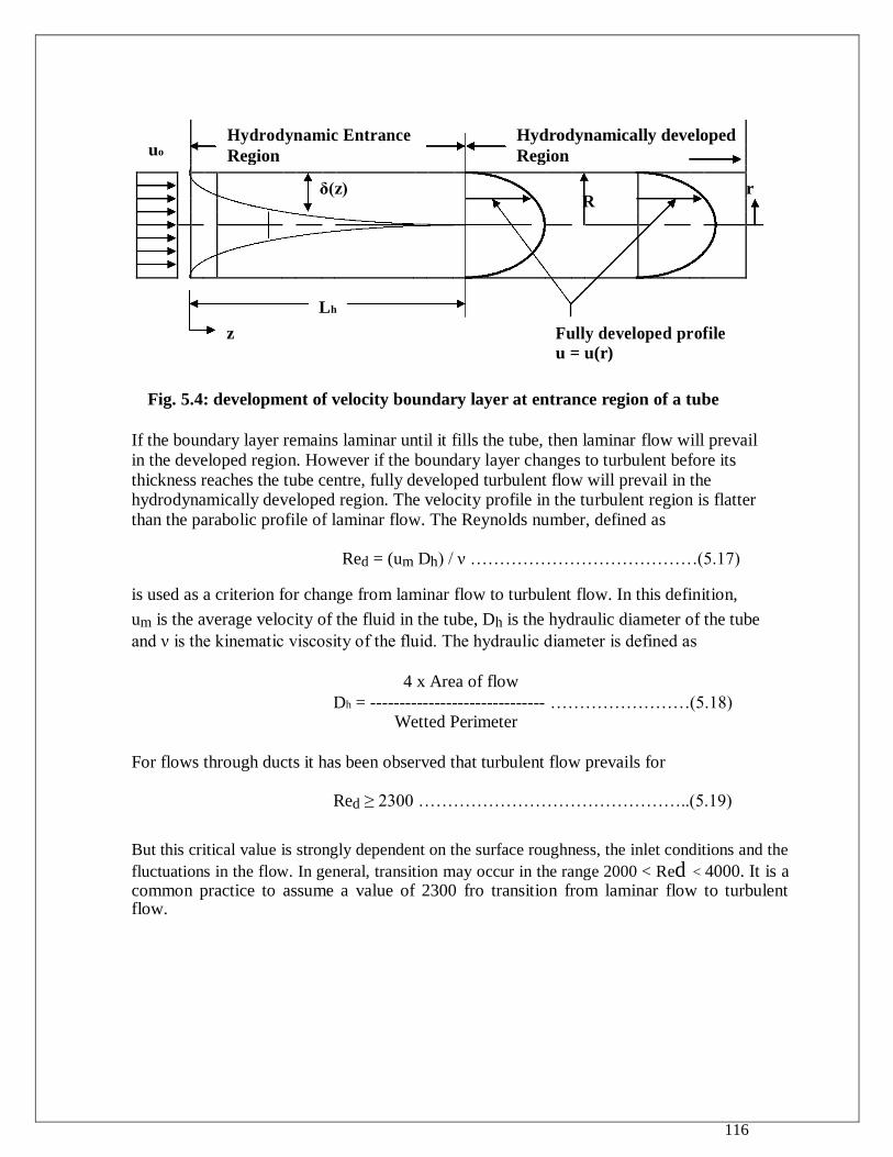
116

uo Hydrodynamic Entrance Hydrodynamically developed

Region Region

r

δ(z) R

Lh

z Fully developed profile

u = u(r)

Fig. 5.4: development of velocity boundary layer at entrance region of a tube

If the boundary layer remains laminar until it fills the tube, then laminar flow will prevail

in the developed region. However if the boundary layer changes to turbulent before its

thickness reaches the tube centre, fully developed turbulent flow will prevail in the hydrodynamically developed region. The velocity profile in the turbulent region is flatter

than the parabolic profile of laminar flow. The Reynolds number, defined as

Red = (um Dh) / ν …………………………………(5.17)

is used as a criterion for change from laminar flow to turbulent flow. In this definition,

um is the average velocity of the fluid in the tube, Dh is the hydraulic diameter of the tube

and ν is the kinematic viscosity of the fluid. The hydraulic diameter is defined as

4 x Area of flow Dh = ------------------------------ ……………………(5.18)

Wetted Perimeter

For flows through ducts it has been observed that turbulent flow prevails for

Red ≥ 2300 ………………………………………..(5.19)

But this critical value is strongly dependent on the surface roughness, the inlet conditions and the

fluctuations in the flow. In general, transition may occur in the range 2000 < Red < 4000. It is a common practice to assume a value of 2300 fro transition from laminar flow to turbulent flow.

117

5.4.2. Friction Factor and Pressure Drop Relations For Hydrodynamically Developed

Laminar Flow

In engineering applications, the pressure gradient (dp / dz) associated with the flow is a

quantity of interest, because this decides the pumping power required to overcome thr frictional losses in the pipe of a given length.

Consider a differential length dz of the tube at a distance z from the entrance and

let this length be in the fully developed region. The various forces acting on the fluid element in the direction of flow are shown in Fig.5.5.

Resultant force in the direction of motion = F = (pA)z –(pA)z+dz – ηw Sdz

where S is the perimeter of the duct.

Using Taylor‟s series expansion and neglecting higher order terms we can write

(pA)z+dz = (pA)z + d/dz(pA) dz

Therefore F = d/dz(pA) dz − ηw Sdz

Rate of change of momentum in the direction of flow = 0 because the velocity u does not vary with respect to z in the fully developed region.

Hence d/dz(pA) dz − ηw Sdz = 0

For duct of uniform cross section A is constant. Therefore the above equation reduces to

dp/dz = − ηw S /A ……………………………….(5.20)

For laminar flow ηw = − μ (du / dr)|wall. Hence Eq. (5.20) reduces to

dp μS ------ = -------- (du/dr)|wall ……………………….(5.21)

dz A

Eq.(5.21) is not practical for the determination of (dp/dz), because it requires the evaluation f the velocity gradient at the wall. Hence for engineering applications a parameter called

“friction factor, f ” is defined as follows:

(dp/dz) Dh

f = − ------------------- ………………………….(5.22a)

½ (ρum2)

Substituting for (dp/dz) from Eq. (5.21) we have

(μS/A) (du/dr)|wall Dh

f = − ---------------------------- …………………..(5.22b)

½ (ρum2)

118

For a circular tube S = πDi, and A = πDi2 / 4. Hence Dh = Di

Hence for a circular tube Eq. (5.22b) reduces to

8μ

f = − ------- (du/dr)|wall …………………………(5.22c)

(ρum2)

Also from Eq. (5.22a) we have

(½ ) (ρum2) f

dp = − ----------------- dz

Dh

Integrating the above equation over a total length L of the tube we have

p2 (½ ) (ρum2) f L

∫dp = − ------------------- ∫dz

p1 Dh 0

or pressure drop = Δp = (p1 – p2) = ( ½ ) (L/Dh) f ρum2 …………………………(5.23)

.

Pumping power is given by P = V Δp ………………………………………...(5.24)

.

where V = volume flow rate of the fluid.

5.4.3. Thermal Boundary Layer: In the case of temperature distribution in flow inside a

tube, it is more difficult to visualize the development of thermal boundary layer and the

existence of thermally developed region. However under certain heating or cooling

conditions such as constant wall-heat flux or constant wall-temperature it is possible to have

thermally developed region. Consider a laminar flow inside a circular tube subjected to uniform heat

flux at the wall. Let „r‟ and „z‟ be the radial and axial coordinates respectively and T(r,z) be the local fluid temperature. A dimensionless temperature θ(r,z) is defined as

T(r,z) – Tw(z)

θ(r,z) = ------------------- ………………………………..(5.25a)

Tm(z) – Tw(z)

where Tw(r,z) = Tube wall-temperature and Tm(z) = Bulk mean temperature of the fluid. The bulk mean temperature at any cross section „z‟ is defined as follows:

∫ ρ(2πrdr) u(r,z) Cp T(r,z) ∫ rdr u(r,z)T(r,z)

Tm(z) = --------------------------------- = ---------------------- ………………..(5.25b) ∫ ρ(2πrdr) u(r,z) Cp ∫ rdr) u(r,z)

119

At the tube wall it is clear that θ(r,z) = 0 and attains some finite value at the centre of the tube. Thus we can visualize the development of thermal boundary layer along the tube

surface as shown in Fig. 5.5.The thickness of the thermal boundary layer δt continuously

grows along the tube surface until it fills the entire tube. The region from the tube inlet to the hypothetical location where the thermal boundary layer thickness reaches the tube centre is called the “thermal entry section”. In this region the shape of the dimensionless temperature profile θ(r,z) changes both in axial and in radial directions. The region beyond the thermal entry section is called as the “thermally developed region”, because in this region the dimensionless temperature profile θ remains invariant with respect to z. That is in this region θ = θ(r).It is difficult to explain qualitatively why θ should be independent of z even though the temperature of the fluid T depends both on r and z. However it can be shown mathematically that, for both constant wall-heat flux and constant wall-temperature conditions, θ depends only on r for large values of z.For constant wall-heat flux condition the

wall-temperature Tw(z) increases with z.

Tw(z) Tw(z) Tw(z)

Tfi

Thermally Developing Region Thermaly

Developed Region Thermal Entrance Length Lth

θ = θ(r)

Fig. 5.5: Development of Thermal Boundary Layer In a Flow

Through A Tube Subjected to Constant Wall-Heat Flux Condition

The variation of wall-temperature and the bulk fluid temperature as we proceed along the length of the tube for constant wall-heat flux conditions is shown in Fig. 5.6.

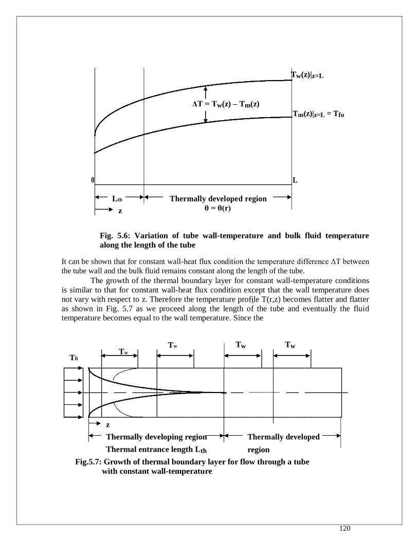
120

Tw(z)|z=L

ΔT = Tw(z) – Tm(z)

Tm(z)|z=L = Tfo

0 L

Lth Thermally developed region

z θ = θ(r)

Fig. 5.6: Variation of tube wall-temperature and bulk fluid temperature

along the length of the tube

It can be shown that for constant wall-heat flux condition the temperature difference ΔT between

the tube wall and the bulk fluid remains constant along the length of the tube. The growth of the thermal boundary layer for constant wall-temperature conditions

is similar to that for constant wall-heat flux condition except that the wall temperature does

not vary with respect to z. Therefore the temperature profile T(r,z) becomes flatter and flatter

as shown in Fig. 5.7 as we proceed along the length of the tube and eventually the fluid temperature becomes equal to the wall temperature. Since the

Tw

Tw Tw Tw

Tfi

z

Thermally developing region Thermally developed

Thermal entrance length Lth region

Fig.5.7: Growth of thermal boundary layer for flow through a tube

with constant wall-temperature

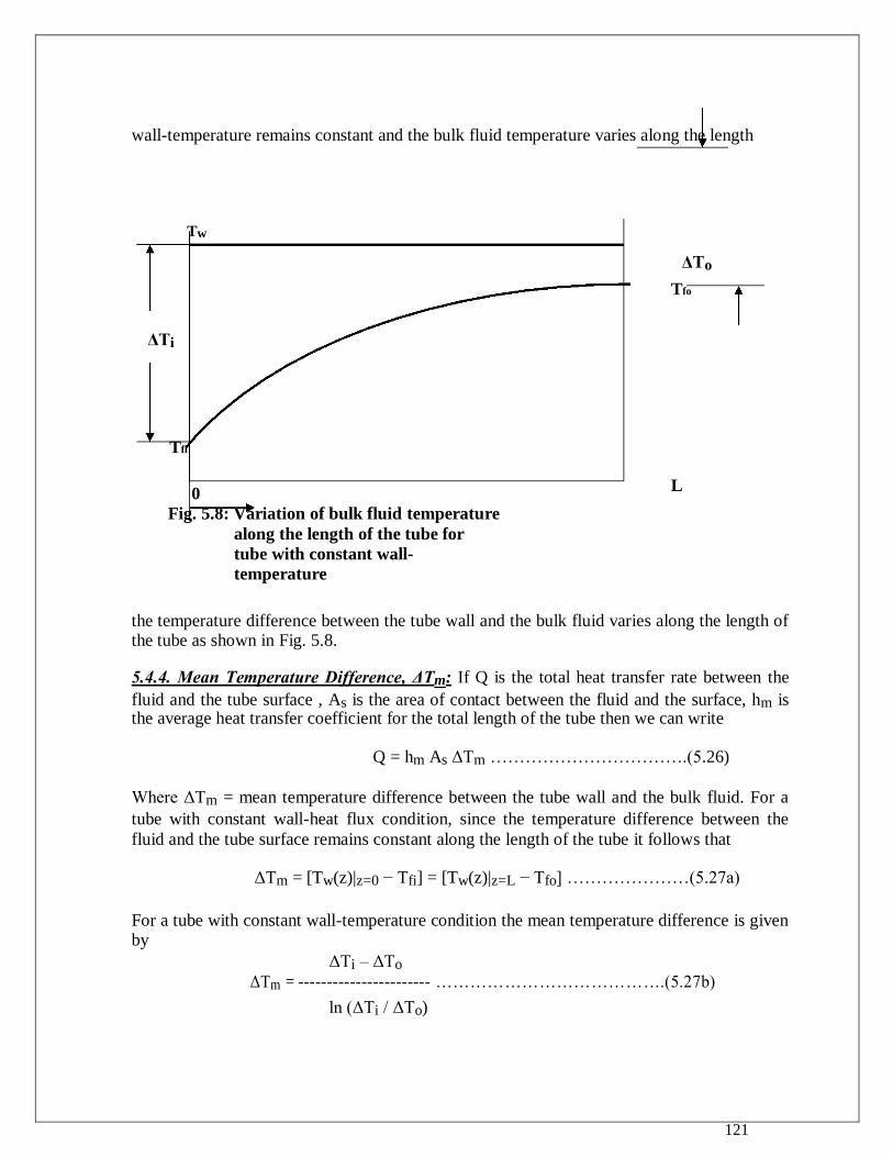
121

wall-temperature remains constant and the bulk fluid temperature varies along the length

Tw

ΔTi

Tfi

0

Fig. 5.8: Variation of bulk fluid temperature

along the length of the tube for

tube with constant wall-

temperature

the temperature difference between the tube wall and the bulk fluid varies along the length of the tube as shown in Fig. 5.8.

5.4.4. Mean Temperature Difference, ΔTm: If Q is the total heat transfer rate between the

fluid and the tube surface , As is the area of contact between the fluid and the surface, hm is the average heat transfer coefficient for the total length of the tube then we can write

Q = hm As ΔTm …………………………….(5.26)

Where ΔTm = mean temperature difference between the tube wall and the bulk fluid. For a

tube with constant wall-heat flux condition, since the temperature difference between the

fluid and the tube surface remains constant along the length of the tube it follows that

ΔTm = [Tw(z)|z=0 − Tfi] = [Tw(z)|z=L − Tfo] …………………(5.27a)

For a tube with constant wall-temperature condition the mean temperature difference is given by

ΔTi – ΔTo

ΔTm = ----------------------- ………………………………….(5.27b)

ln (ΔTi / ΔTo)

ΔTo

Tfo

L

122

123

Free Convective Heat Transfer

A. Free convection from/to plane surfaces:

7.1. A vertical plate 30 cm high and 1 m wide and maintained at a uniform

temperature of 120 0 C is exposed to quiescent air at 30 0 C.Calculate the average heat transfer coefficient and the total heat transfer rate from the plate to air.

7.2. An electrically heated vertical plate of size 25 cm x 25 cm is insulated on one side and dissipates heat from the other surface at a constant rate of 600

W/m2 by free convection into quiescent atmospheric air at 30 0 C. Determine the surface temperature of the plate.

7.3. Determine the heat transfer by free convection from a plate 30 cm x 30 cm

whose surfaces are maintained at 100 0 C and exposed to quiescent air at 20 0 C for the following conditions: (a) the plate is vertical. (b) Plate is horizontal

7.4. A circular plate of 25 cm diameter with both surfaces maintained at a uniform

temperature of 100 0 C is suspended in horizontal position in atmospheric air

at 20 0 C. Determine the heat transfer from the plate.

7.5. Consider an electrically heated plate 25 cm x 25 cm in which one surface is thermallt insulated and the other surface is dissipating heat by free

convection into atmospheric air at 30 0 C. The heat flux over the surface is

uniform and results in a mean surface temperature of 50 0 C. The plate is

inclined making an angle of 50 0 from the vertical. Determine the heat loss from the plate for (i) heated surface facing up and (ii) heated surface facing down.

7.6. A thin electric strip heater of width 20 cm is placed with its width oriented vertically. It dissipates heat by free convection from both the surfaces into

atmospheric air at 20 0 C. If the surface temperature of the heater is not to

exceed 225 0 C, determine the length of the heater required in order to dissipate 1 kW of energy into the atmospheric air.

7.7. A plate 75 cm x 75 cm is thermally insulated on the one side and subjected to

a solar radiation flux of 720 W/m2 on the other surface. The plate makes an

angle of 60 0 with the vertical such that the hot surface is facing upwards. If

the surface is exposed to quiescent air at 25 0 C and if the heat transfer is by pure free convection determine the equilibrium temperature of the plate.

B. Free convection from/to Cylinders:

7.8. A 5 cm diameter, 1.5 m long vertical tube at a uniform temperature of 100 0C

is exposed to quiescent air at 20 0 C. calculate the rate of heat transfer from the surface to air. What would be the heat transfer rate if the tube were kept horizontally?

7.9. A horizontal electrical cable of 25 mm diameter has a heat dissipation rate of

30 W/m. If the ambient air temperature is 27 0 C, estimate the surface temperature of the cable.

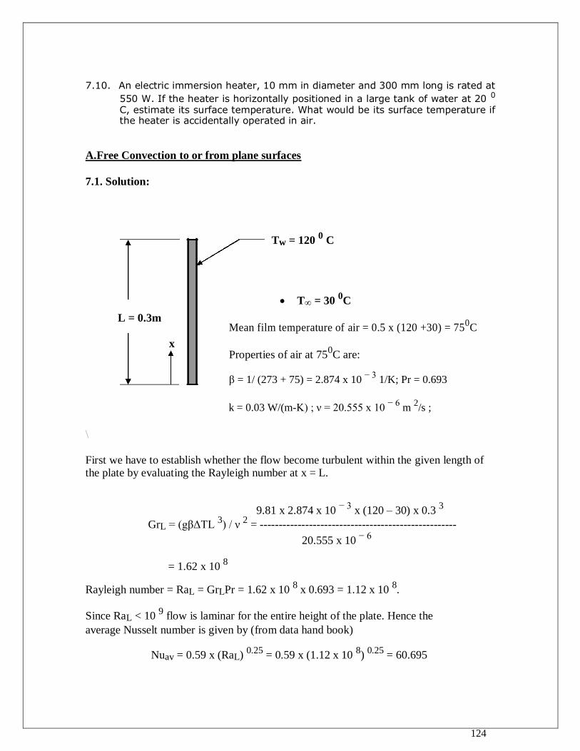
124

7.10. An electric immersion heater, 10 mm in diameter and 300 mm long is rated at

550 W. If the heater is horizontally positioned in a large tank of water at 20 0 C, estimate its surface temperature. What would be its surface temperature if the heater is accidentally operated in air.

A.Free Convection to or from plane surfaces

7.1. Solution:

Tw = 120 0 C

T∞ = 30 0C

L = 0.3m Mean film temperature of air = 0.5 x (120 +30) = 75

0C

x

Properties of air at 750C are:

β = 1/ (273 + 75) = 2.874 x 10 − 3

1/K; Pr = 0.693

k = 0.03 W/(m-K) ; ν = 20.555 x 10 − 6

m 2/s ;

\

First we have to establish whether the flow become turbulent within the given length of the plate by evaluating the Rayleigh number at x = L.

9.81 x 2.874 x 10 − 3

x (120 – 30) x 0.3 3

GrL = (gβΔTL 3) / ν

2 = ----------------------------------------------------

20.555 x 10 − 6

= 1.62 x 10 8

Rayleigh number = RaL = GrLPr = 1.62 x 10 8 x 0.693 = 1.12 x 10

8.

Since RaL < 10 9 flow is laminar for the entire height of the plate. Hence the

average Nusselt number is given by (from data hand book)

Nuav = 0.59 x (RaL) 0.25

= 0.59 x (1.12 x 10 8)

0.25 = 60.695

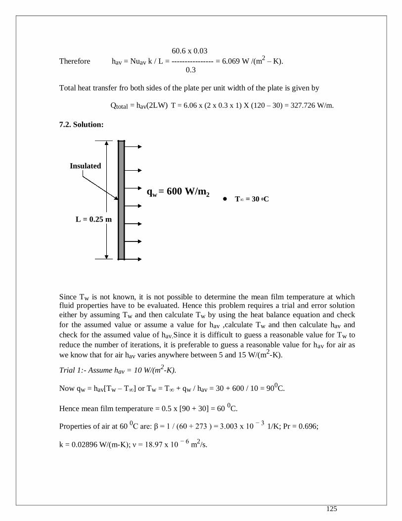
125

60.6 x 0.03

Therefore hav = Nuav k / L = ---------------- = 6.069 W /(m2 – K).

0.3

Total heat transfer fro both sides of the plate per unit width of the plate is given by

Qtotal = hav(2LW) T = 6.06 x (2 x 0.3 x 1) X (120 – 30) = 327.726 W/m.

7.2. Solution:

Insulated

qw

= 600 W/m2 T∞ = 30 0C

L = 0.25 m

Since Tw is not known, it is not possible to determine the mean film temperature at which fluid properties have to be evaluated. Hence this problem requires a trial and error solution

either by assuming Tw and then calculate Tw by using the heat balance equation and check

for the assumed value or assume a value for hav ,calculate Tw and then calculate hav and

check for the assumed value of hav.Since it is difficult to guess a reasonable value for Tw to

reduce the number of iterations, it is preferable to guess a reasonable value for hav for air as

we know that for air hav varies anywhere between 5 and 15 W/(m2-K).

Trial 1:- Assume hav = 10 W/(m2-K).

Now qw = hav[Tw – T∞] or Tw = T∞ + qw / hav = 30 + 600 / 10 = 900C.

Hence mean film temperature = 0.5 x [90 + 30] = 60 0C.

Properties of air at 60 0C are: β = 1 / (60 + 273 ) = 3.003 x 10

− 3 1/K; Pr = 0.696;

k = 0.02896 W/(m-K); ν = 18.97 x 10 − 6

m2/s.

126

9.81 x 3.003 x 10 − 3

x 600 x (0.25)4

RaL* = GrL*Pr =[(gβqwx

4) /(kν

2)]Pr = ---------------------------------------------- x 0.696

0.02896 x (18.97 x 10 − 6

) 2

Or RaL* = 4.61 x 10

9.

Since RaL * >10

9 flow is turbulent for the entire length of the plate

Hence Nuav = 1.25 Nux|x=L = 1.25 x 0.17 x (4.61 x 10 9)

0.2 = 55.37

Therefore hav = 55.37 x 0.02896 / 0.25 = 6.41 W/(m2 – K)

Since the calculated value of hav deviates from the assumed value by about 34 %,

one more iteration is required.

Trial 2:- Assume hav = 6.41 W/(m2-K)

Hence Tw = 30 + 600 / 6.41 = 123.6 0C 120

0 C

Mean film temperature = 0.5 x (120 + 30) = 75 0 C

Properties of air at 75 0C are:- β = 1/(75 + 273) = 2.873 x 10

− 3 1/K. Pr =

0.686 k = 0.03338 W /(m-K); ν = 25.45 x 10 − 6

m 2 /s.

9.81 x 2.873 x 10 − 3

x 600 x 0.25 4

R aL* = ------------------------------------------- x 0.686 = 2.06 x 10 9

0.03338 x (25.45 x 10 − 6

) 2

Flow is turbulent for the entire length of the plate.

Hence Nuav = 1.25 Nux|x=L = 1.25 x 0.17 x (2.06 x 10 9)

0.25 = 45.27

Therefore hav = 45.27 x 0.03338 / 0.25 = 6.04 W/(m2 – K).

Since the calculated value of hav is very close to the assumed value, the iteration

is stopped. The surface temperature of the plate is therefore given by

Tw = 30 + 600 / 6.04 = 129.3 0 C.

7.3. Solution:- Case(i) When the plate is vertical

Data:- Characteristic length = L = height of the plate = 0.3 m; Tw = 100 0C;T∞= 20

0C; Mean film temperature = 0.5 x (100 + 20) = 60

0C.

127

Properties of air at 60 0C are: β = 1 / (60 + 273 ) = 3.003 x 10

− 3 1/K; Pr = 0.696;

k = 0.02896 W/(m-K); ν = 18.97 x 10 − 6

m2/s.

RaL = GrLPr =( gβΔTL 3/ ν

2) Pr

9.81 x 3.003 x 10 − 3

x (100 – 20) x (0.3) 3

= ---------------------------------------------------- x 0.696

(18.97 x 10 − 6

) 2

= 1.23 x 10 8

From data hand book corresponding to this value of RaL have

Nuav = 0.59 x (1.23 x 10 8)

0.25 = 62.13

Therefore hav = 62.13 x 0.02896 / 0.3 = 5.99 W/(m2-K).

Rate of heat transfer = Q = hav(2LW)(ΔT) = 5.99 x (2 x 0.3 x 0.3) x (100 – 20)

= 86.256 W

128

UNIT-IV

Condensation & Boiling

Introduction: Knowledge of heat transfer occurring during change of phase i.e. during

condensation and boiling is very useful in a number of ways. For example in all power and

refrigeration cycles, it is necessary to convert a liquid into a vapour and vice-versa. This is

accomplished in boilers or evaporators and condensers. Heat transfer coefficients in both condensation and boiling are generally

much higher than those encountered in single phase processes. Values greater than 1000

W/(m2-K) are almost always obtained. This fact has been used in several recent applications

where it is desired to transfer high heat fluxes with modest temperature differences. An example is the “heat pipe” which is a device capable of transferring a large quantity of heat with very small temperature differences.

8.2. Film-wise and Drop-wise condensation:- Condensation occurs whenever a vapour

comes into contact with a surface at a temperature lower than the saturation temperature of

the vapour corresponding to its vapour pressure. The nature of condensation depends on

whether the liquid thus formed wets the solid surface or does not wet the surface. If the liquid

wets the surface, the condensate flows on the surface in the form of a film and the process is

called “film-wise condensation”. If on the other hand, the liquid does not wet the surface, the

condensate collects in the form of droplets, which either grow in size or coalesce with

neighboring droplets and eventually roll of the surface under the influence of gravity. This

type of condensation is called “drop-wise condensation”.

The rate of heat transfer during the two types of condensation processes

is quite different. For the same temperature difference between the vapour and the surface,

the heat transfer rates in drop-wise condensation are significantly higher than those in film-

wise condensation. Therefore it is preferable to have drop-wise condensation from the

designer‟s point of view if the thermal resistance on the condensing side is a significant part

of the total thermal resistance. However it is generally observed that, although drop-wise

condensation may be obtained on new surfaces, it is difficult to maintain drop-wise

condensation continuously and prolonged condensation results in a change to film-wise

condensation. Therefore it is still the practice to design condensers under the conservative

assumption that the condensation is of film type.

8.3. Nusselt’s theory for laminar film-wise condensation on a plane vertical surface:-The problem of laminar film-wise condensation on a plane vertical surface was first analytically

solved by Nusselt in 1916.He made the following simplifying assumptions in his analysis. (i) The fluid properties are constant.

(ii) The plane surface is maintained at a uniform temperature, Tw which is less than the

saturation temperature Tv of the vapour.

(iii) The vapour is stationary or has a very low velocity and so it does not exert any drag on the motion of the condensate: i.e., the shear stress at the liquid-vapour interface is zero. (iv) The flow velocity of the condensate layer is so low that the acceleration of the condensate is negligible. (v) The downward flow of the condensate under the action of gravity is laminar. (vi) Heat transfer across the condensate layer is purely by conduction; hence the liquid temperature distribution is linear.

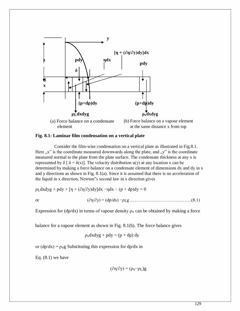
129

y

[η + (∂η/∂y)dy]dx

x pdy ηdx pdy

δ

d

x

(p+dp)dy

(p+dp)dy

ρLdxdyg ρvdxdyg

(a) Force balance on a condensate

element

(b) Force balance on a vapour element

at the same distance x from top

Fig. 8.1: Laminar film condensation on a vertical plate

Consider the film-wise condensation on a vertical plate as illustrated in Fig.8.1.

Here „x‟ is the coordinate measured downwards along the plate, and „y‟ is the coordinate

measured normal to the plate from the plate surface. The condensate thickness at any x is

represented by δ [ δ = δ(x)]. The velocity distribution u(y) at any location x can be

determined by making a force balance on a condensate element of dimensions dx and dy in x

and y directions as shown in Fig. 8.1(a). Since it is assumed that there is no acceleration of

the liquid in x direction, Newton‟s second law in x direction gives

ρLdxdyg + pdy + [η + (∂η/∂y)dy]dx −ηdx − (p + dp)dy = 0

or (∂η/∂y) = (dp/dx) −ρLg …………………………………..(8.1)

Expression for (dp/dx) in terms of vapour density ρv can be obtained by making a force

balance for a vapour element as shown in Fig. 8.1(b). The force balance gives

ρvdxdyg + pdy = (p + dp) dy

or (dp/dx) = ρvg Substituting this expression for dp/dx in

Eq. (8.1) we have

(∂η/∂y) = (ρv−ρL)g

130

Since the flow is assumed to be laminar, η = μL(∂u/∂y)

Therefore ∂/∂y{μL (∂u/∂y)} = (ρv−ρL)g

Integrating with respect to y we have μL (∂u/∂y) = (ρv−ρL)g y + C1

(ρv−ρL)g y C1 Or (∂u/∂y) = --------------- + ------- ……(8.2)

μL μL

Integrating once again with respect to y we get

(ρv−ρL)g y2

C1 y

u(y) = ---------------- + ------------- + C2 ...... (8.3)

2 μL μL

The boundary conditions for the condensate layer are: (i) at y = 0, u = 0;

(ii) at y = δ, (∂u/∂y) = 0.

Condition (i) in Eq. (8.3) gives C2 = 0 and condition (ii) in Eq. (8.2) gives

(ρv−ρL)g δ C1

0 = ------------- + ---------

2 μL μL

(ρv−ρL)g δ

Therefore C1 = − -------------- 2

Substituting for C1 and C2 in Eq.(8.3) we get the velocity distribution in the

condensate layer as

g(ρL − ρv)

u(y) = --------------- [ δy – (y2/2)] …………………(8.4)

μL

If „m‟ is the mass flow rate of the condensate at any x then

δ

m = 0∫ρLudy

δ

m = 0∫ ρL{ g(ρL − ρv) / μL}[ δy – (y2/2)]dy

131

g ρL (ρL − ρv) δ 3

= ------------------ ………………………………..(8.5)

3 μL

g ρL (ρL − ρv) δ 2 dδ

Hence dm = ----------------------

μL

Amount of heat transfer across the condensate element = dq = dm hfg

g ρL (ρL − ρv) δ 2 dδ hfg

Or dq = ------------------------- ………………………….(8.6)

μL

Energy balance for the condensate element shown in the figure can be written as

dq = kL(Tv – Tw)dx / δ

g ρL (ρL − ρv) δ 2 dδ hfg

Or ------------------------- = kL(Tv – Tw)dx / δ………….(8.6)

μL

kL μL (Tv – Tw)dx

or δ 3dδ = ----------------------

g ρL (ρL − ρv) hfg

Integrating we get

δ 4 kL μL (Tv – Tw)x

----- = --------------------- + C 3

4 g ρL (ρL − ρv) hfg

At x = 0, δ = 0. Hence C3 = 0.

Therefore δ 4 kL μL (Tv – Tw)x

----- = ---------------------

4 g ρL (ρL − ρv) hfg

4 kL μL (Tv – Tw)x

or δ = [-------------------------- ] 1/ 4

……………………(8.7)

g ρL (ρL − ρv) hfg

132

Now kL (Tv – Tw)dx

----------------- = hx dx [Tv – Tw]

δ

kL g ρL (ρL − ρv) hfg kL3

Therefore hx = --------- = [ -------------------------- ] 1 / 4

δ 4 μL (Tv – Tw)x

g ρL (ρL − ρv) hfg kL3

Or hx = 0.707[ --------------------------] 1 / 4

............................... (8.8)

μL (Tv – Tw)x

The local Nusselt number Nux can therefore be written as

hxx g ρL (ρL − ρv) hfg x3

Nux = ----- = 0.707[ --------------------------] 1 / 4

............................... (8.8)

kL μL (Tv – Tw)kL

The average heat transfer coefficient for a length L of the plate is given by

L hav = (1/L) ∫ hxdx ………………………………………(8.9)

0

It can be seen from Eq. (8.8) that hx = C x − ¼

, where C is a constant given by

g ρL (ρL − ρv) hfg kL3

Or C = 0.707[ --------------------------] 1 / 4

…………………(8.10)

μL (Tv – Tw)

Hence hav = (1/L) C ∫ x − ¼

dx = (C / L) (4/3) L− ¼

= (4/3)C L− ¼

0

Substituting for C from Eq. (8.10) we have

g ρL (ρL − ρv) hfg kL3

hav = 0.943[ --------------------------] 1 / 4

= (4/3)hx|x = L.........................(8.11)

μL (Tv – Tw)L

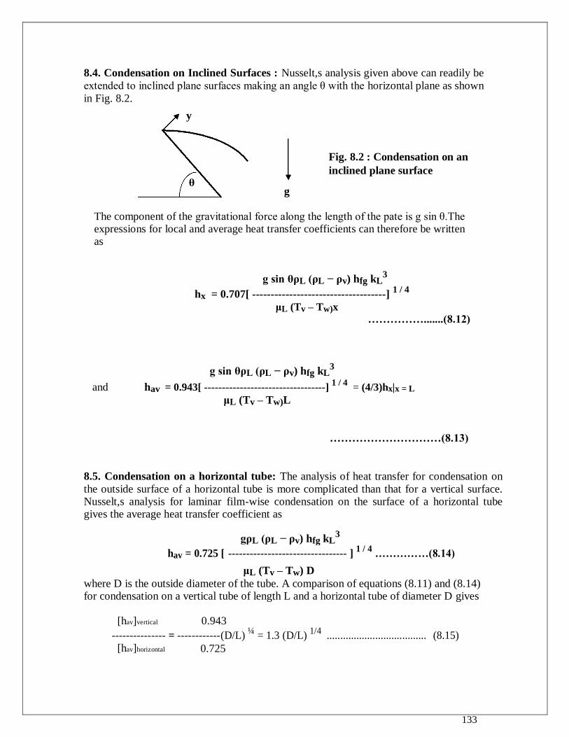
133

8.4. Condensation on Inclined Surfaces : Nusselt,s analysis given above can readily be

extended to inclined plane surfaces making an angle θ with the horizontal plane as shown

in Fig. 8.2.

y

θ

Fig. 8.2 : Condensation on an inclined plane surface

g

The component of the gravitational force along the length of the pate is g sin θ.The expressions for local and average heat transfer coefficients can therefore be written as

g sin θρL (ρL − ρv) hfg kL3

hx = 0.707[ ------------------------------------] 1 / 4

μL (Tv – Tw)x

…………….......(8.12)

g sin θρL (ρL − ρv) hfg kL3

and hav = 0.943[ ----------------------------------] 1 / 4

= (4/3)hx|x = L

μL (Tv – Tw)L

…………………………(8.13)

8.5. Condensation on a horizontal tube: The analysis of heat transfer for condensation on

the outside surface of a horizontal tube is more complicated than that for a vertical surface. Nusselt,s analysis for laminar film-wise condensation on the surface of a horizontal tube gives the average heat transfer coefficient as

gρL (ρL − ρv) hfg kL3

hav = 0.725 [ --------------------------------- ] 1 / 4

……………(8.14)

μL (Tv – Tw) D

where D is the outside diameter of the tube. A comparison of equations (8.11) and (8.14) for condensation on a vertical tube of length L and a horizontal tube of diameter D gives

[hav]vertical 0.943

--------------- = ------------(D/L) ¼

= 1.3 (D/L) 1/4

..................................... (8.15)

[hav]horizontal 0.725

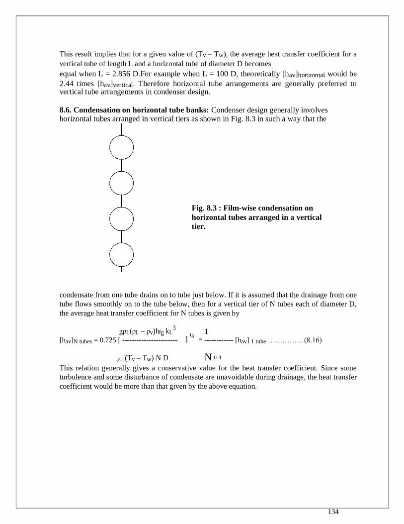
134

This result implies that for a given value of (Tv – Tw), the average heat transfer coefficient for a

vertical tube of length L and a horizontal tube of diameter D becomes

equal when L = 2.856 D.For example when L = 100 D, theoretically [hav]horizontal would be

2.44 times [hav]vertical. Therefore horizontal tube arrangements are generally preferred to vertical tube arrangements in condenser design.

8.6. Condensation on horizontal tube banks: Condenser design generally involves horizontal tubes arranged in vertical tiers as shown in Fig. 8.3 in such a way that the

Fig. 8.3 : Film-wise condensation on horizontal tubes arranged in a vertical tier.

condensate from one tube drains on to tube just below. If it is assumed that the drainage from one

tube flows smoothly on to the tube below, then for a vertical tier of N tubes each of diameter D,

the average heat transfer coefficient for N tubes is given by

gρL(ρL – ρv)hfg kL3

] ¼

= 1

[hav]N tubes = 0.725 [ ----------------------- ------------ [hav] 1 tube ……………(8.16)

μL(Tv – Tw) N D N 1/ 4

This relation generally gives a conservative value for the heat transfer coefficient. Since some

turbulence and some disturbance of condensate are unavoidable during drainage, the heat transfer

coefficient would be more than that given by the above equation.

135

8.7. Reynolds number for condensate flow: Although the flow hardly changes to turbulent

flow during condensation on a single horizontal tube, turbulence may start at the lower

portions of a vertical tube. When the turbulence occurs in the condensate film, the average

heat transfer coefficient begins to increase with the length of the tube in contrast to its

decrease with the length for laminar film condensation. To establish a criterion for transition

from laminar to turbulent flow, a “Reynolds number for condensate flow” is defined as

follows. ρL uav Dh

Re = ----------------- …………………..(8.17)

μL

where uav is the average velocity of the condensate film and Dh is the hydraulic

diameter for the condensate flow given by

4 x (Cross sectional area for condensate flow) 4A

Dh = --------------------------------------------- --------- = -------

Wetted Perimeter P

4A ρL uav 4M

Therefore Re = -------------------- = --------------- ……………..(8.18)

P μL P μL

where M is mass flow rate of condensate at the lowest part of the condensing surface

in kg/s. The wetted perimeter depends on the geometry of the condensing surface and is given as follows.

πD …..For vertical tube of outside diameter D ………….(8.19 a) P = 2L …...For horizontal tube of length L …………………(8.19 b)

W ….. For vertical or inclined plate of width W………...(8.19 c)

Experiments have shown that the transition from laminar to turbulent condensation

takes place at a Reynolds number of 1800. The expression for average heat transfer coefficient for a vertical surface [Eq.(8.11)] can be expressed as follows.

136

g ρL(ρL – ρv) kL3 hfg

hav = 0.943 [ ----------------------------- ] 1 / 4

μL(Tv – Tw)

Generally ρL >> ρv. Therefore

g ρL2 kL

3 hfg

hav = 0.943 [ ----------------------------- ] 1 / 4

………………..(8.20)

μL(Tv – Tw)

The above equation can be arranged in the form

hav [νL2 / (gkL

3) ]

1 / 3 = 1.47 Re L

− 1/ 3 ………………………(8.21)

The above equation is valid for ReL < 1800.

It has been observed experimentally that when the value of the film Reynolds number is greater than 30, there are ripples on the film surface which increase the value of the heat transfer coefficient. Kutateladze has proposed that the value of the local heat

transfer coefficient be multiplied by 0.8(RE / 4)0.11

to account for the ripples effect.

Using this correction it can be shown that

(hav / kL)( νL2 / g)

1 / 3 =

ReL

------------------------ ………………(8.22)

[1.08 ReL1.22

– 5.2]

8.8. Turbulent film condensation: For turbulent condensation on a vertical surface,

Kirkbride has proposed the following empirical correlation based on experimental data.

hav [νL2 / (gkL

3) ]

1 / 3 = 0.0077 (ReL)

0.4 ……………………(8.23)

In the above correlation the physical properties of the condensate should be evaluated at

the arithmetic mean temperature of Tv and Tw.

8.9. Film condensation inside horizontal tubes: In all the correlations mentioned above, it

is assumed that the vapour is either stationary or has a negligible velocity. In practical

applications such as condensers in refrigeration and air conditioning systems, vapour

condenses on the inside surface of the tubes and so has a significant velocity. In such

situations the condensation phenomenon is very complicated and a simple analytical

treatment is not possible. Consider, for example, the film condensation on the inside surface

of a long vertical tube.

137

The upward flow of vapour retards the condensate flow and causes thickening of the

condensate layer, which in turn decreases the condensation heat transfer coefficient.

Conversely the down ward flow of vapour decreases the thickness of the condensate film and

hence increases the heat transfer coefficient.

Chato recommends the following correlation for condensation at low vapour velocities inside horizontal tubes:

g ρL(ρL – ρv) kL3 h*fg

hav = 0.555 [ --------------------------- ] 1 / 4

……………..(8.24 –a)

μL(Tv – Tw) D

where h*fg = hfg + (3/8)cp,L(Tv – Tw) ………………………….(8.24 –b)

This result has been developed for the condensation of refrigerants at low Reynolds number [Rev

= (ρvuvD) / μv < 35,000 ; Rev should be evaluated at the inlet conditions.]

For higher flow rates, Akers, Deans and Crosser propose the following correlation for the average condensation heat transfer coefficient on the inside surface of a

horizontal tube of diameter D:

hav D

------ = 0.026 Pr 1 / 3

[ReL + Rev(ρL / ρv) ½

] 0.8

………..(8.25)

k

where ReL = (4ML) / (πDμL) : Rev = (4Mv) / (πDμv) …………………….(8.26)

The above equation correlates the experimental data within 50 % for ReL > 5000

and Rev > 20,000.

8.10. Illustrative examples on film wise condensation:

Example 8.1: Saturated steam at 1.43 bar condenses on a 1.9 cm OD vertical tube which is

20 cm long. The tube wall is at a uniform temperature of 109 0C . Calculate the average heat

transfer coefficient and the thickness of the condensate film at the bottom of the tube.

Solution: Data:- Tv = Saturation temperature at 1.43 bar = 110 0 C (from steam tables)

Tw = 109 0C ; Characteristic length = L = 0.2 m ; D = 0.019 m ;

To find : (i) hav ; (ii) δ(x)|x=L;

Mean film temperature of the condensate (water) = 0.5 x (110 + 109) = 109.5 0C.

Properties of water at 109.5 0C are: ρL = 951.0 kg/m

3; μL = 258.9 x 10

− 6 N-s / m

2; k

= 0.685 W/(m-K); ν = 0.2714 x 10 − 6

m2/s; hfg = 2230 kJ/kg. Also ρL >>> ρv.

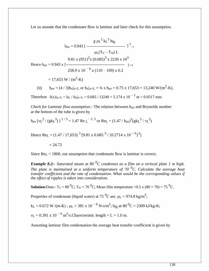
138

Let us assume that the condensate flow is laminar and later check for this assumption.

g ρL2 kL

3 hfg

] 1 / 4

hav = 0.943 [ -----------------------------

μL(Tv – Tw) L

9.81 x (951)2x (0.685)

3 x 2230 x 10

3

Hence hav = 0.943 x [-------------------------------------------- ] 1/ 4

258.9 x 10 − 6

x (110 – 109) x 0.2

= 17,653 W / (m2-K)

(ii) hav = (4 / 3)hx|x=L or hx|x=L = ¾ x hav = 0.75 x 17,653 = 13,240 W/(m2-K).

Therefore δ(x)|x=L = kL / hx|x=L = 0.685 / 13240 = 5.174 x 10 − 5 m = 0.0517 mm.

Check for Laminar flow assumption:- The relation between hav and Reynolds number

at the bottom of the tube is given by

hav [νL2 / (gkL

3) ]

1 / 3 = 1.47 Re L

− 1/ 3 or ReL = (1.47 / hav)

3(gkL

3 / νL

2)

Hence ReL = (1.47 / 17,653) 3 [9.81 x 0.685

3 / {0.2714 x 10

− 6}

2]

= 24.72

Since ReL < 1800, our assumption that condensate flow is laminar is correct.

Example 8.2:- Saturated steam at 80 0C condenses as a film on a vertical plate 1 m high.

The plate is maintained at a uniform temperature of 70 0C. Calculate the average heat

transfer coefficient and the rate of condensation. What would be the corresponding values if the effect of ripples is taken into consideration.

Solution:Data:- Tv = 80 0C; Tw = 70

0C; Mean film temperature =0.5 x (80 + 70) = 75

0C.

Properties of condensate (liquid water) at 75 0C are: ρL = 974.8 kg/m

3;

kL = 0.672 W /(m-K) ; μL = 381 x 10 − 6

N-s/m2; hfg at 80

0C = 2309 kJ/kg-K;

νL = 0.391 x 10 − 6

m2/s.Charecteristic length = L = 1.0 m.

Assuming laminar film condensation the average heat transfer coefficient is given by

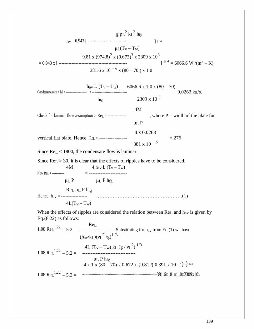
139

g ρL2 kL

3 hfg

hav = 0.943 [ ----------------------------- ] 1 / 4

μL(Tv – Tw)

9.81 x (974.8)2 x (0.672)

3 x 2309 x 10

3

= 0.943 x [ ------------------------------------------------ ] 1/ 4

= 6066.6 W /(m2 – K).

381.6 x 10 − 6

x (80 – 70 ) x 1.0

hav L (Tv – Tw) 6066.6 x 1.0 x (80 – 70) Condensate rate = M = --------------------- = ------------------------------- 0.0263 kg/s.

hfg 2309 x 10 3

4M

Check for laminar flow assumption :- ReL = -------------- , where P = width of the plate for

μL P

4 x 0.0263

vertical flat plate. Hence ReL = ------------------------- = 276

381 x 10 − 6

Since ReL < 1800, the condensate flow is laminar.

Since ReL > 30, it is clear that the effects of ripples have to be considered.

4M 4 hav L (Tv – Tw)

Now ReL = ------------ = -----------------------

μL P μL P hfg

ReL μL P hfg

Hence hav = ------------------ …………………………………………….(1)

4L(Tv – Tw)

When the effects of ripples are considered the relation between ReL and hav is given by Eq.(8.22) as follows:

1.08 ReL1.22

ReL

– 5.2 = ----------------------- Substituting for hav from Eq.(1) we have

(hav/kL)(νL2 /g)

1 /3

1.08 ReL1.22

– 5.2 =

4L (Tv – Tw) kL (g / νL2)

1/3

--------------------------------

μL P hfg − 6)2}1/3

1.08 ReL1.22

4 x 1 x (80 – 70) x 0.672 x {9.81 /( 0.391 x 10

– 5.2 = ----------------------------------------------------------------------381.6x10−6x1.0x2309x103

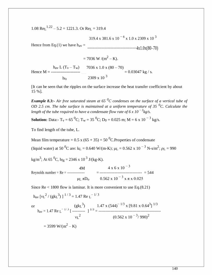
140

1.08 ReL1.22

– 5.2 = 1221.3. Or ReL = 319.4

319.4 x 381.6 x 10 − 6

x 1.0 x 2309 x 10 3

Hence from Eq.(1) we have hav = ----------------------------------------------------4x1.0x(80–70)

= 7036 W /(m2 – K).

hav L (Tv – Tw) 7036 x 1.0 x (80 – 70)

Hence M = --------------------- = --------------------- ------- = 0.03047 kg / s.

hfg 2309 x 10 3

[It can be seen that the ripples on the surface increase the heat transfer coefficient by about 15 %].

Example 8.3:- Air free saturated steam at 65 0C condenses on the surface of a vertical tube of

OD 2.5 cm. The tube surface is maintained at a uniform temperature of 35 0C. Calculate the

length of the tube required to have a condensate flow rate of 6 x 10 −3kg/s.

Solution: Data:- Tv = 65 0C; Tw = 35

0C; D0 = 0.025 m; M = 6 x 10

− 3 kg/s.

To find length of the tube, L.

Mean film temperature = 0.5 x (65 + 35) = 50 0C.Properties of condensate

(liquid water) at 50 0C are: kL = 0.640 W/(m-K); μL = 0.562 x 10

− 3 N-s/m

2; ρL = 990

kg/m3; At 65

0C, hfg = 2346 x 10

3 J/(kg-K).

4M 4 x 6 x 10 − 3

Reynolds number = Re = --------------- = ------------------------------- = 544

μL πDo 0.562 x 10 − 3

x π x 0.025

Since Re < 1800 flow is laminar. It is more convenient to use Eq.(8.21)

hav [νL2 / (gkL

3) ]

1 / 3 = 1.47 Re L

− 1/ 3

or (gkL3) 1.47 x (544)

− 1/3 x [9.81 x 0.64

3]

1/3

hav = 1.47 Re L− 1/ 3

[ ---------- ] 1/3

= ----------------------------------------------

νL2

(0.562 x 10 − 3

/ 990)2

= 3599 W/(m2 – K)

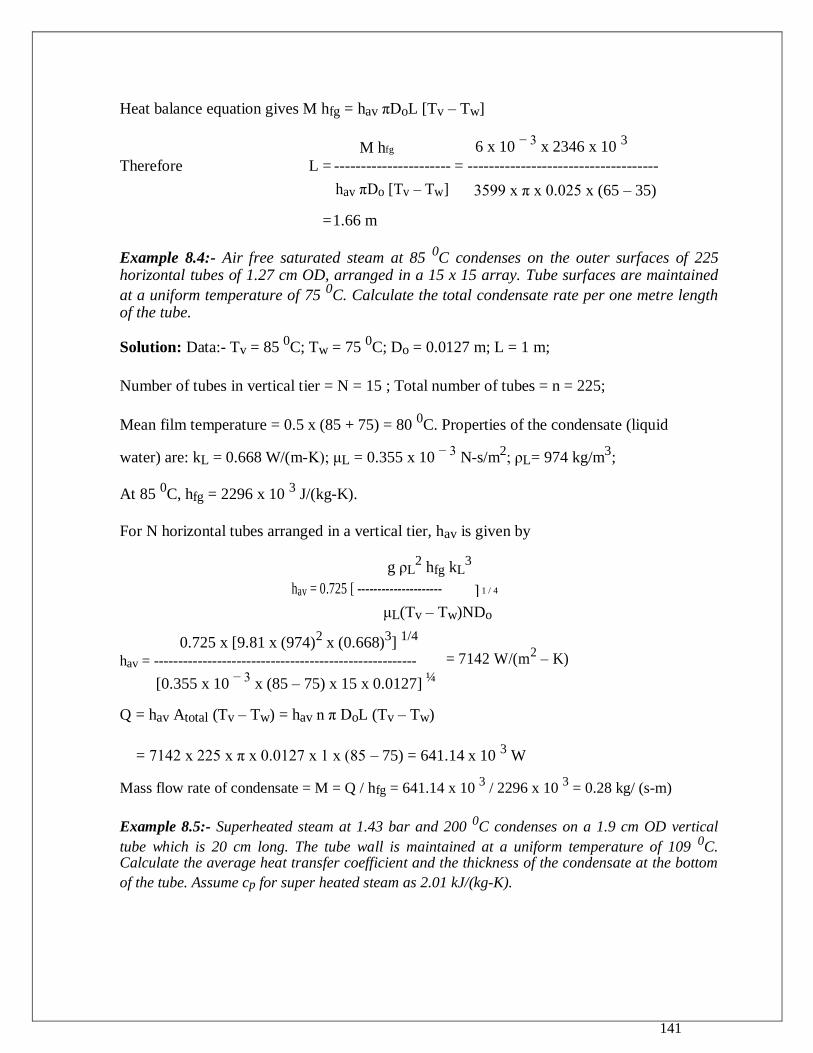
141

Heat balance equation gives M hfg = hav πDoL [Tv – Tw]

M hfg 6 x 10 − 3

x 2346 x 10 3

Therefore L = ---------------------- = ------------------------------------

hav πDo [Tv – Tw] 3599 x π x 0.025 x (65 – 35)

= 1.66 m

Example 8.4:- Air free saturated steam at 85 0C condenses on the outer surfaces of 225

horizontal tubes of 1.27 cm OD, arranged in a 15 x 15 array. Tube surfaces are maintained

at a uniform temperature of 75 0C. Calculate the total condensate rate per one metre length

of the tube.

Solution: Data:- Tv = 85 0C; Tw = 75

0C; Do = 0.0127 m; L = 1 m;

Number of tubes in vertical tier = N = 15 ; Total number of tubes = n = 225;

Mean film temperature = 0.5 x (85 + 75) = 80 0C. Properties of the condensate (liquid

water) are: kL = 0.668 W/(m-K); μL = 0.355 x 10 − 3

N-s/m2; ρL= 974 kg/m

3;

At 85 0C, hfg = 2296 x 10

3 J/(kg-K).

For N horizontal tubes arranged in a vertical tier, hav is given by

g ρL2 hfg kL

3

hav = 0.725 [ --------------------- ] 1 / 4

μL(Tv – Tw)NDo

0.725 x [9.81 x (974)2 x (0.668)

3]

1/4

= 7142 W/(m2 – K)

hav = ------------------------------------------------------

[0.355 x 10 − 3

x (85 – 75) x 15 x 0.0127] ¼

Q = hav Atotal (Tv – Tw) = hav n π DoL (Tv – Tw)

= 7142 x 225 x π x 0.0127 x 1 x (85 – 75) = 641.14 x 10 3 W

Mass flow rate of condensate = M = Q / hfg = 641.14 x 10 3 / 2296 x 10

3 = 0.28 kg/ (s-m)

Example 8.5:- Superheated steam at 1.43 bar and 200 0C condenses on a 1.9 cm OD vertical

tube which is 20 cm long. The tube wall is maintained at a uniform temperature of 109 0C. Calculate the average heat transfer coefficient and the thickness of the condensate at the bottom

of the tube. Assume cp for super heated steam as 2.01 kJ/(kg-K).

142

Solution: With a superheated vapour, condensation occurs only when the surface

temperature is less than the saturation temperature corresponding to the vapour pressure.

Therefore for a superheated vapour, the amount of heat to be removed per unit mass to condense it is given by

Q / M = hfg + cpv(Tv – Tsat)

Where cp is the specific heat of superheated steam and Tsat is the saturation temperature

corresponding to the vapour pressure. If it is assumed that the liquid – vapour interphase is at the

saturation temperature, then Eq.(8.20 ) still holds good with hfg replaced by

hfg + cpv(Tv – Tsat).

Hence g ρL2 kL

3 { hfg + cpv(Tv – Tsat)}

hav = 0.943 [ --------------------------------------- ] 1/ 4

μL(Tsat – Tw)L

At 1.43 bar, Tsat = 110 0C.Mean film temperature = 0.5 x (110 + 109) = 109.5

0C.

Properties of the condensate at 109.5 0C are: kL = 0.685W/(m-K); μL = 0.259 x 10

− 3 N-

s/m2; ρL= 951 kg/m

3;At 1.43 bar, hfg = 2230 x 10

3 J/(kg-K).

9.81 x (951)2 x (0.685)

3x {2230 x 10

3 + 2010 x (200 – 110)}

hav = 0.943 x [ -------------------------------------------------------------------------- ] 1/ 4

0.259 x 10 − 3

x (110 – 109) x 0.2

= 18,000 W /(m2 – K).

Hence hx|x=L = (¾) x 18000 = 13,500 W / (m2 – K).

δ(x)|x=L = kL / hx|x=L = 0.685 / 13,500 = 5.07 x 10 − 5

m

Example 8.6:- Air free saturated steam at 70 0C condenses on the outer surface of a 2.5 cm

OD vertical tube whose outer surface is maintained at a uniform temperature of

50 0C. What length of the tube would produce turbulent film condensation?

Solution: Data:- Tv = 70 0C; Tw = 50

0C; Do = 0.025 m; Vertical tube.

To find L such that Re = 1800.

Mean film temperature = 0.5 x (70 + 50) = 60 0C. Properties of the condensate (liquid

water) are : kL = 0.659W/(m-K); μL = 0.4698 x 10 − 3

N-s/m2; ρL= 983.2 kg/m

3;

143

At 70 0C hfg = 2358 x 10

3 J/(kg-K).

Re (μLπDo) 1800 x 0.4698 x 10 − 3

x π x 0.025

Re = 4M / (μLπDo) or M = ------------------- = ---------------------------------------------

4 4

= 0.0166 kg / s.

For turbulent flow hav [νL2 / (gkL

3) ]

1 / 3 = 0.0077 (ReL)

0.4

Or hav = 0.0077 (ReL) 0.4

[νL2 / (gkL

3) ]

− 1 / 3

Hence hav = 0.0077 x (1800)0.4

x [ (0.4698 x 10 − 3

/983.2)2 / (9.81 x 0.659

3) ]

−

1 / 3 = 3563.4 W / (m

2 – K).

Heat balance equation is M hfg = hav π DoL (Tv – Tw)

M hfg 0.0166 x 2358 x 10 3

Hence L = ----------------------- = -------------------------------------

hav π Do (Tv – Tw) 3563.4 x π x 0.025 x (70 – 50)

= 7 m

Example 8.7:- Saturated steam at 100 0C condenses on the outer surface of a 2 m long

vertical plate. What is the temperature of the plate below which the condensing film at the bottom of the plate will become turbulent?

Solution: Data:- Tv = 100 0C; L = 2 m. Since Tw is not known, properties of the condensate

at the mean film temperature cannot be determined and therefore the problem has to be

solved by trial and error procedure as follows:

Trial 1:- The properties of the condensate are read at Tv = 100 0C. The properties

are kL = 0.683 W/(m-K); μL = 0.2824 x 10 − 3

N-s/m2; ρL= 958.4 kg/m

3; At 100

0C,

hfg = 2257 x 10 3 J/kg-K.

Since the flow has to become turbulent at the bottom of the plate we have

hav = 0.0077 (ReL) 0.4

[νL2 / (gkL

3) ]

− 1 / 3 with ReL = 1800

144

9.81 x 0.683 3

Hence hav = 0.0077 x (1800)0.4

x [ ------------------------------ ] 1 / 3

(0.2824 x 10 − 3

/ 958.4) 2

= 5098 W / (m2 – K)

Now M hfg = hav L W (Tv – Tw)

Or Tw = Tv – (M/W)hfg / (hav L). But ReL = 4M / (μLW) or M/W = ReL μL / 4.

ReL μL hfg 1800 x 0.2824 x 10 − 3

x 2257 x 10 3

Therefore Tw = Tv − -------------------- = 100 − ----------------------------------------------

4 hav L 4 x 5098 x 2

= 72 0C

Trial 2:- Assume Tw = 72 0C. Mean film temperature = 0.5 x (100 + 72) = 86

0C. Properties

of the condensate at 86 0C ; kL = 0.677 W/(m-K); μL = 0.3349 x 10

− 3 N-s/m

2;

ρL= 968.5kg/m3; At 100

0C, hfg = 2257 x 10

3 J/(kg-K).

9.81 x 0.677 3

Hence hav = 0.0077 x (1800)0.4

x [ ------------------------------ ] 1 / 3

(0.3349 x 10 − 3

/ 968.5) 2

= 4541 W /(m2 – K).

1800 x 0.3349 x 10 − 3

x 2257 x 10 3

= 60 0C

Therefore Tw = 100 − -----------------------------------------------

4 x 4541 x 2

Since the calculated value of Tw is quite different from the assumed value, one more iteration

is required.

Trial 3:- Assuming Tw = 60 0C and proceeding on the same lines as shown in trial 2 we

get hav = 4365 W /(m2 – K) and hence Tw = 59

0C. This value is very close to the value

assumed (difference is within 2 % ). The iteration is stopped. Hence Tw = 59 0C.

Example 8.8:- Air free saturated steam at 90 0C condenses on the outer surface of a 2.5 cm

OD, 6 m long vertical tube, whose outer surface is maintained at a uniform temperature of

60 0C. Calculate the total rate of condensation of steam at the tube surface.

145

Solution: Data:- Tv = 90 0C; Tw = 30

0C; Do = 0.025 m; L = 6 m. Vertical tube.

Mean film temperature = 0.5 x (90 + 60) = 75 0C. Properties of the condensate at 75

0C

are: kL = 0.671 W/(m-K); μL = 0.3805 x 10 − 3

N-s/m2; ρL= 974.8 kg/m

3; At 90

0C, hfg

= 2283 x 10 3 J/(kg-K).

We do not know whether the condensate flow is laminar or turbulent. We start the calculations assuming laminar flow and then check for laminar flow condition. For laminar flow

g ρL2 kL

3 hfg

] 1 / 4

hav = 0.943 [ -----------------------------

μL(Tv – Tw) L

9.81 x (974.8)2 x (0.671)

3 x 2283 x 10

3

Hence hav = 0.943 x [-------------------------------------------------- ] 1 / 4

0.3805 x 10 − 3

x (90 – 60) x 6

= 2935.3 W /(m2 – K).

For laminar flow hav [νL2 / (gkL

3) ]

1 / 3 = 1.47 Re L

− 1/ 3

Or ReL = (1.47 / hav)3(gkL

3 / νL

2)

= (1.47 / 2935.3)3 x [9.81 x 0.671

3 x 974.8

2 / (0.3805 x 10

− 3)2]

= 2443

Since ReL > 1800, flow is turbulent.

For turbulent flow hav [νL2 / (gkL

3) ]

1 / 3 = 0.0077 (ReL)

0.4

Or hav = 0.0077 (ReL) 0.4

/ [νL2 / (gkL

3) ]

1 / 3……….(1)

ReL = 4M / (μLπDo). But Mhfg = havπDoL (Tv – Tw) or M / (πDo) = havL (Tv – Tw) / hfg

4 havL (Tv – Tw)

Therefore ReL = ----------------------

hfg μL

Substituting this expression for ReL in equation (1) we have

146

4 havL (Tv – Tw)

] 0.4 [νL2 / (gkL

3) ]

− 1 / 3

hav = 0.0077 [-------------------------

hfg μL

4 L (Tv – Tw)

(hav )0.6

= 0.0077 [------------------------- ] 0.4

[νL2 / (gkL

3) ]

− 1 / 3

hfg μL

4 x 6 x (90 – 60) (0.3805 x 10 − 3

)2

= 0.0077 x [--------------------------------------- ] 0.4

x [ --------------------------------- ] − 1 / 3

2283 x 10 3 x 0.3805 x 10

− 3 974.8

2 x 9.81 x (0.671)

3

= 192. Hence hav = [192] 1 / 0.6

= 6390 W /(m2 – K).

havπDoL (Tv – Tw) 6390 x π x 0.025 x 6 x(90 – 60)

Therefore M = ----------------------- = - - - - - -- - - - - - -- - - - - - -- - - - - -- - - - - - -- - - - - -- - -

2283 x 10 3

= 0.0396 kg/s

hfg

8.11. Dropwise Condensation: Experimental investigations on condensation have indicated

that, if traces of oil are present in steam and the condensing surface is highly polished, the

condensate film breaks into droplets. This type of condensation is called “drop wise

condensation”. The droplets grow, coalesce and run off the surface, leaving agreater portion

of the condensing surface exposed to the incoming steam. Since the entire condensing

surface is not covered with a continuous layer of liquid film, the heat transfer rate for ideal

drop wise condensation is much higher than that for film wise condensation. The heat transfer coefficient may be 2 to 3 times greater for drop wise condensation than for

film wise condensation. Hence considerable research has been done with the objective of

producing long lasting drop wise condensation. Various types of chemicals have been tried to

promote drop wise condensation. Continuous drop wise condensation, obtainable with

different promoters varies between 100 to 300 hours with pure steam and are shorter with

industrial steam. Failure occurs because of fouling or oxidation of the surface, or by the flow

of the condensate or by a combination of these effects. It is unlikely that long lasting drop wise condensation can be produced under

practical conditions by a single treatment of any of the promoters currently available. Therefore

in the analysis of a heat exchanger involving condensation of steam, it is recommended that film

wise condensation be assumed for the condensing surface.

8.12. Boiling Types: When evaporation occurs at a solid-liquid interface, it is called as

“boiling”. The boiling process occurs when the temperature of the surface Tw exceeds the

saturation temperature Tsat corresponding to the liquid pressure. Heat is transferred from the solid surface to the liquid, and the appropriate form of Newton‟s law of cooling is

qw = h [Tw – Tsat] = h ∆Te …………………………(8.27)

147

Where ∆Te = [Tw - Tsat] and is termed as the “excess temperature”. The boiling process is

characterized by the formation of vapour bubbles which grow and subsequently detach from the surface. Vapour bubble growth and dynamics depend, in a complicated manner, on the

excess temperature ∆Te, the nature of the surface, and the thermo-physical properties of the

fluid, such as its surface tension. In turn the dynamics of vapour bubble growth affect fluid motion near the surface and therefore strongly influence the heat transfer coefficient.

Boiling may occur under varying conditions. For example if the liquid is

quiescent and if its motion near the surface is due to free convection and due to mixing

induced by bubble growth and detachment, then such a boiling process is called “pool

boiling”. In contrast in “forced convection boiling”, the fluid motion is induced by an

external means as well as by free convection and bubble induced mixing. Boiling may also

be classified as “sub-cooled boiling” and “saturated boiling”. In sub-cooled boiling, the

temperature of the liquid is below the saturation temperature and the bubbles formed at the

surface may condense in the liquid. In contrast, in saturated boiling, the temperature of the

liquid slightly exceeds the saturation temeperature, Bubbles formed at the surface are then

propelled through the liquid by buoyancy forces, eventually escaping from a free surface.

8.13. Pool Boiling Regimes: The first investigator who established experimentally the different regimes of pool boiling was Nukiyama. He immersed an electric resistance wire into a body of saturated water and initiated boiling on the surface of the wire by passing electric current through it. He determined the heat flux as well as the temperature from the measurements of current and voltage. Since the work of Nukiyama, a number of investigations on pool boiling have been reported. Fig. 8.4 illustrates the characteristics of pool boiling for water at atmospheric pressure. This boiling curve illustrates the variation of heat flux or the heat transfer coefficient as a

function of excess temperature ∆Te. This curve pertains to water at 1 atm pressure.From Eq.

(8.27) it can seen that qw depends on the heat transfer coefficient h and the excess temperature

∆Te.

Free Convection Regime(up to point A):- Free convection is said to exist if ∆Te ≤ 5 0 C. In

this regime there is insufficient vapour in contact with the liquid phase to cause boiling at the

saturation temperature. As the excess temperature is increased, the bubble inception will

eventually occur, but below point A (referred to as onset of nucleate boiling,ONB), fluid motion is primarily due to free convection effects.Therefore,according to whether

the flow is laminar or turbulent, the heat transfer coefficient h varies as ∆Te1/4

or as ∆Te1/3

respectively so that qw varies as ∆Te5/4

or as ∆Te4/3

.

Nucleate Boiling Regime(Between points A and C):- Nucleate boiling exists in the range 5 0 C ≤

∆Te ≤ 30 0 C. In this range, two different flow regimes may be distinguished. In the region A –

B, isolated bubbles form at nucleation sites and separate from the surface, substantially

increasing h and qw. In this regime most of the heat exchange is through direct transfer from the surface to liquid in motion at the surface, and not through vapour bubbles rising from the

surface. As ∆Te is increased beyond 10 0C (Region B-C), the nucleation sites will be

numerous and the bubble generation rate is so high that continuous columns of vapour appear. As a result very high heat fluxes are obtainable in this region. In practical applications, the nucleate boiling regime is most desirable, because large heat fluxes are obtainable with small temperature differences. In the nucleate boiling regime, the heat increases rapidly with increasing excess temperature

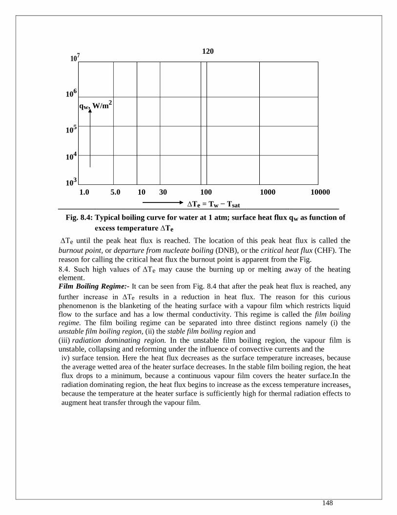
148

107

120

106

qw, W/m2

105

104

103

1.0 5.0 10 30 100 1000 10000

∆Te = Tw − Tsat

Fig. 8.4: Typical boiling curve for water at 1 atm; surface heat flux qw as function of

excess temperature ∆Te

∆Te until the peak heat flux is reached. The location of this peak heat flux is called the

burnout point, or departure from nucleate boiling (DNB), or the critical heat flux (CHF). The

reason for calling the critical heat flux the burnout point is apparent from the Fig.

8.4. Such high values of ∆Te may cause the burning up or melting away of the heating element. Film Boiling Regime:- It can be seen from Fig. 8.4 that after the peak heat flux is reached, any

further increase in ∆Te results in a reduction in heat flux. The reason for this curious

phenomenon is the blanketing of the heating surface with a vapour film which restricts liquid

flow to the surface and has a low thermal conductivity. This regime is called the film boiling regime. The film boiling regime can be separated into three distinct regions namely (i) the

unstable film boiling region, (ii) the stable film boiling region and (iii) radiation dominating region. In the unstable film boiling region, the vapour film is unstable, collapsing and reforming under the influence of convective currents and the iv) surface tension. Here the heat flux decreases as the surface temperature increases, because

the average wetted area of the heater surface decreases. In the stable film boiling region, the heat

flux drops to a minimum, because a continuous vapour film covers the heater surface.In the

radiation dominating region, the heat flux begins to increase as the excess temperature increases,

because the temperature at the heater surface is sufficiently high for thermal radiation effects to

augment heat transfer through the vapour film.

149

8.14. Pool Boiling Correlations:

Correlation for The Nucleate Boiling Regime:- The heat transfer in the nucleate

boiling regime is affected by the nucleation process, the distribution of active nucleation

sites on the surface, and the growth and departure of bubbles.Numerous experimental

investigations have been reported and a number of attempts have been made to correlate

the experimental data corresponding to nucleate boiling regime.The most successful and

widely used correlation was developed by Rohsenow. By analyzing the significance of

various parameters in relation to forced - convection effects. He proposed the following

empirical relation to correlate the heat flux in the entire nucleate boiling regime:

Cpl ∆Te

------------- = Csf

hfg Prln

qw _______________

[ --------- √ ζ* / {g (ρl – ρv)} ] 0.33

………………. (8.28)

(μl hfg)

where Cpl = specific heat of saturated liquid, J /(kg -0C)

Csf = constant to be determined from experimental data depending

upon Heating surface – fluid combination

hfg = latent heat of vapourization, J / kg

g = acceleration due to gravity, m / s2

Prl = Prandtl number of saturated liquid

qw = boiling heat flux, W / m2

∆Te = excess temperature as defined in Eq. (8.27)

μl = viscosity of saturated liquid, kg / (m – s)

ρl, ρv = density of liquid and saturated vapour respectively, kg /

m3 ζ

* = surface tension of liquid – vapour interface, N / m.

In Eq. (8.28) the exponent n and the coefficient Csf are the two provisions to adjust the

correlation for the liquid – surface combination. Table 8-1 gives the experimentally determined

values Csf for a variety of liquid – surface combinations. The value of n should be taken as 1 for

water and 1.7 for all other liquids shown in Table 8 – 1.

150

Example 8.10:- A metal clad heating element of 6 mm diameter and emissivity equal to unity

is horizontally immersed in a water bath. The surface temperature of the metal is 255 0C

under steady state boiling conditions. If the water is at atmospheric pressure estimate the power dissipation per unit length of the heater.

Solution: Given:- Tw = 255 0C ; Tsat = saturation temperature of water at 1 atm = 100

0C;

∆Te = 255 – 100 = 155 0C. Since ∆Te > 120

0C, film boiling conditions will prevail.

The heat transfer in this regime is given by Eq.(8.33) namely

kv3 ρv (ρl – ρv) g hfg

*

ho = 0.62 [ ----------------------------------- ] ¼

D μv ∆Te

Properties of water at 100 0C are: ρl = 957.9 kg/m

3; hfg = 2257 x 10

3 J/kg;

ρv = 4.808 kg/m3; Cpv = 2.56 x 10

3 J/(kg-K); kv = 0.0331 W / (m-

0C);

μv = 14.85 x 10 − 6

kg / (m-s).

Substituting these values in the expression for ho we have

3 3 3

(0.0331) x 4.808 x (957.9 – 4.808) x 9.81 x {2257 x 10 + 0.8 x 2.56 x 10 x 155 }

ho = 0.62 x [---------------------------------------------------------------------- 14.85 x 10

− 6 x 0.006 x 155

] ¼

= 460 W/(m2 – K)

1 ζ {Tw4 – Tsat

4}

hr = ---------------------- x ------------------------------

[1/ε + 1/α − 1 ] {Tw – Tsat}

1 5.67 x 10 − 8

x { 528 4 – 373

4}

= ------------------------ x -------------------------------------------

[ 1 / 1 + 1 / 1 − 1 ] { 528 – 373}

= 21.3 W / (m2-K).

Now h ≈ ho + ¾ hr = 460 + ¾ x 21.3 = 476 W /(m2 – K).

Hence Q = h A ∆Te = 476 x (π x 0.006 x 1)x 155 = 1.36 x 10 3 W / m.

Example 8.11:- A vessel with a flat bottom and 0.1 m2 in area is used for boiling water at

atmospheric pressure. Find the temperature at which the vessel must be maintained if a boiling rate of 80 kg/h is desired. Assume that the vessel is made of copper and the boiling is

nucleate boiling. Take ρv = 0.60 kg/m3.

151

Solution: Given:- A = 0.1 m2; Tsat = 100

0C; M = 80 kg/h = 0.022 kg/s; Prl = 1.75

hfg = 2257 x10 3 J /kg; Cpl = 4216 J/(kg-K); ρl = 960.6 kg/m

3; ζ* = 58.8 x 10

− 3 N/m;

μl = 282.4 x 10 − 6

kg / (m-s); n = 1; For water-copper combination Csf = 0.0130;

M hfg 0.022 x 2257 x 10 3

qw = Q / A = -------- = ---------------------------- = 4.965 x 10 3 W/m

2

A 0.1

For nucleate boiling Eq.(8.28) is used to calculate the excess temperature .∆Te

Cpl ∆Te qw _______________

------------- = Csf [ --------- √ ζ* / {g (ρl – ρv)} ] 0.33

hfg Prln

(μl hfg)

4216 x ∆Te

2257-----------------------

x103x1.75

= 0.013 x {4.965 x 10 5/(282.4 x 10

− 6x 2257 x 10

3)

_____________________________

x √ 58.8 x 10 − 3

/ [9.81 x (960.6 – 0.6)] } 0.33

Or ∆Te = 15.2 0C

Hence Tw = 100 + 15.2 = 115.2 0C.

152

Example 8.12:- Calculate the heat transfer coefficient during stable film boiling of water

from a 0.9 cm diameter horizontal carbon tube. The water is saturated and at 100 0C and the

tube surface is at 1000 0C. Take the emissivity of the carbon surface to be 0.8 and assume

that at the average film temperature, the steam has the following properties.

kv = 0.0616 W/(m-K); ρv = 0.266 kg/m3; μv = 28.7 x 10

−6 kg/(m-s); Cpv = 2168 J/(kg-K); ρl

= 958.4 kg/m3

Solution: Given:- D = 0.009 m; ∆Te = Tw – Tsat = 1000 – 100 = 900 0C; ε = 0.8; α =

1.0 hfg* = hfg + 0.8 Cpv ∆Te = 2257 x 10

3 + 0.8 x 2168 x 900 = 3818 x 10

3 J/kg.

For stable film boiling the convection coefficient is given by Eq.(8.33)

kv3 ρv (ρl – ρv) g hfg

*

ho = 0.62 [ ----------------------------------- ] ¼

D μv ∆Te

(0.0616)3 x 0.266 x (958.4 – 0.266) x 9.81 x 3818 x 10

3

ho = 0.62 x [ ---------------------------------------------------------------------- ] ¼

0.009x (28.7 x 10 − 6

) x 900

= 194 W/(m2 – K)

Radiation heat transfer coefficient is given by

1 ζ (Tw4 – Tsat

4)

hr = ---------------------- -------------------------

[ 1/ε + 1/α – 1] (Tw – Tsat)

1 5.67 x 10 − 8

(1273 4 − 373

4)

hr = ---------------------- x --------------------------------------

[ 1/0.8 + 1/1 – 1] (1273 – 373)

= 131.4 W/(m2 – K).

Hence h = ho + ¾ hr = 194 + ¾ x 131.4 = 292.5

153

RADIATION HEAT TRANSFER

10.1. INTRODUCTORY CONCEPTS AND DEFINITIONS

10.1.1 THERMAL RADIATION

When a body is placed in an enclosure whose walls are at temperatures below that of the body, the temperature of the body will decrease even if the enclosure is evacuated. This process by which heat is transferred from a body by virtue of its temperature, without the aid of any intervening medium is called “THERMAL RADIATION”. The actual mechanism of radiation is not yet completely understood. There are at present two theories by means of which radiation propagation is explained. According to Maxwell‟s electromagnetic theory, Radiation is treated as electromagnetic waves, while Max Planck‟s theory treats radiation as “Photons” or “Quanta of energy”. Neither theory completely describes all observed phenomena. It is however known that radiation travels

with the speed of light, c (c = 3x108 m/s) in a vacuum. This speed is equal to the product

of the frequency of the radiation and the wavelength of this radiation,

OR c = λν ………………………………….(10.1)

Where λ = wavelength of radiation (m) and ν = frequency (1/s).

Usually, it is more convenient to specify wavelength in micrometer, which is equal

to 10-6

m.

From the viewpoint of electromagnetic wave theory, the waves travel at the speed of light, while from the quantum theory point of view, energy is transported by photons which travel at the speed of light. Although all the photons have the same velocity, there

is always a distribution of energy among them. The energy associated with a photon, ep =

hν where h is the Planck‟s constant equal to 6.6256 x 10-34

Js. The entire energy spectrum can also be described in terms of the wavelength of radiation.

Radiation phenomena are usually classified by their characteristic wavelength, λ.

At temperatures encountered in most engineering applications, the bulk of the thermal

energy emitted by a body lies in the wavelengths between λ= 0.1 and 100 μm. For this

reason, the portion of the wavelength spectrum between λ= 0.1 and 100 μm is generally

referred to as “THERMAL RADIATION”. The wavelength spectrum in the range λ= 0.4

and 0.7 μm is visible to the naked eye, and this is called „light rays‟. The wavelength

spectrum of radiation is illustrated in Fig 10.1

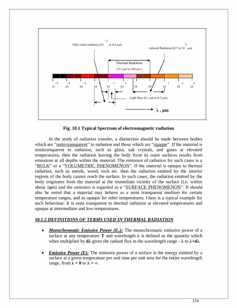
154

−2

Ultra violet radiation (10 to 0.4 μm) 3 Infrared Radiation (0.7 to 10 μm)

Thermal Radiation

( 0.1 μm to 100 μm )

−5 −4 −3 −2 10

−1 0 10 10

2 3 4 5

10 10 10 10 10 10 10 10

Light Rays (0.1 μm to 0.3 μm)

λ , μm

Fig. 10.1 Typical Spectrum of electromagnetic radiation

In the study of radiation transfer, a distinction should be made between bodies

which are “semi-transparent” to radiation and those which are “opaque”. If the material is

semitransparent to radiation, such as glass, salt crystals, and gases at elevated

temperatures, then the radiation leaving the body from its outer surfaces results from

emissions at all depths within the material. The emission of radiation for such cases is a

“BULK” or a “VOLUMETRIC PHENOMENON”. If the material is opaque to thermal

radiation, such as metals, wood, rock etc. then the radiation emitted by the interior

regions of the body cannot reach the surface. In such cases, the radiation emitted by the

body originates from the material at the immediate vicinity of the surface (i.e. within

about 1μm) and the emission is regarded as a “SURFACE PHENOMENON”. It should

also be noted that a material may behave as a semi transparent medium for certain

temperature ranges, and as opaque for other temperatures. Glass is a typical example for

such behaviour. It is semi transparent to thermal radiation at elevated temperatures and

opaque at intermediate and low temperatures.

10.1.2 DEFINITIONS OF TERMS USED IN THERMAL RADIATION

Monochromatic Emissive Power (Eλ): The monochromatic emissive power of a

surface at any temperature T and wavelength λ is defined as the quantity which

when multiplied by dλ gives the radiant flux in the wavelength range - λ to λ+dλ.

Emissive Power (E): The emissive power of a surface is the energy emitted by a surface at a given temperature per unit time per unit area for the entire wavelength range, from λ = 0 to λ = ∞.

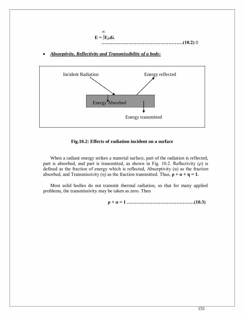
155

∞

E = ∫Eλdλ ……………………………………………(10.2) 0

Absorptivity, Reflectivity and Transmissibility of a body:

Incident Radiation Energy reflected

Energy Absorbed

Energy transmitted

Fig.10.2: Effects of radiation incident on a surface

When a radiant energy strikes a material surface, part of the radiation is reflected,

part is absorbed, and part is transmitted, as shown in Fig. 10.2. Reflectivity (ρ) is defined as the fraction of energy which is reflected, Absorptivity (α) as the fraction

absorbed, and Transmissivity (η) as the fraction transmitted. Thus, ρ + α + η = 1.

Most solid bodies do not transmit thermal radiation, so that for many applied problems, the transmissivity may be taken as zero. Then

ρ + α = 1 ……………………………………(10.3)

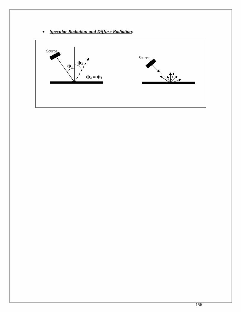
156

Specular Radiation and Diffuse Radiation:

Source

Φ1

Source Φ2

Ф2 = Φ1

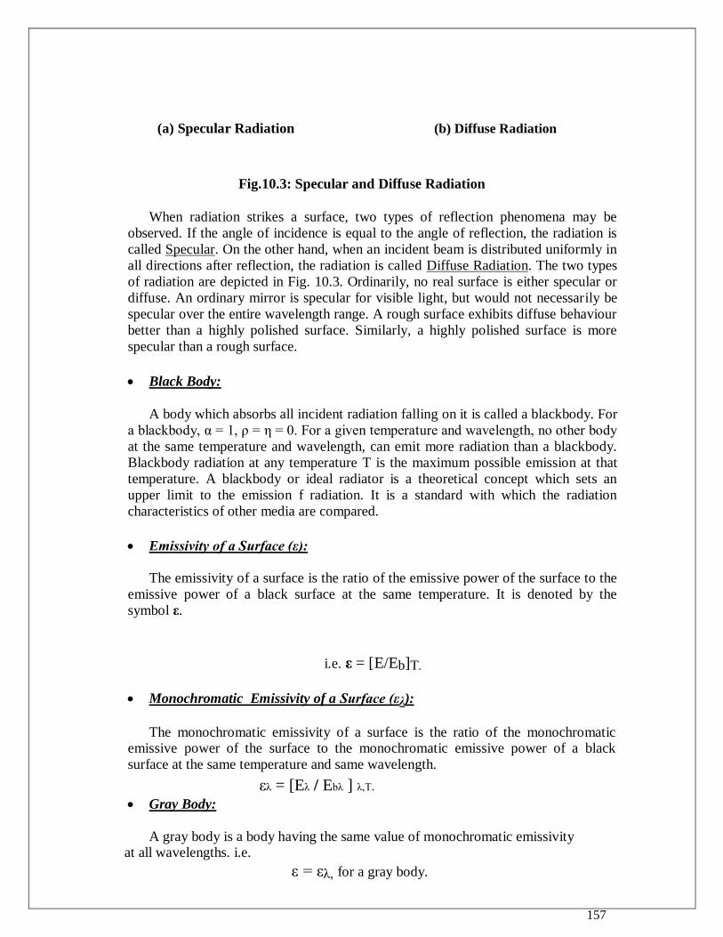
157

(a) Specular Radiation (b) Diffuse Radiation

Fig.10.3: Specular and Diffuse Radiation

When radiation strikes a surface, two types of reflection phenomena may be

observed. If the angle of incidence is equal to the angle of reflection, the radiation is

called Specular. On the other hand, when an incident beam is distributed uniformly in

all directions after reflection, the radiation is called Diffuse Radiation. The two types

of radiation are depicted in Fig. 10.3. Ordinarily, no real surface is either specular or

diffuse. An ordinary mirror is specular for visible light, but would not necessarily be

specular over the entire wavelength range. A rough surface exhibits diffuse behaviour

better than a highly polished surface. Similarly, a highly polished surface is more

specular than a rough surface.

Black Body:

A body which absorbs all incident radiation falling on it is called a blackbody. For

a blackbody, α = 1, ρ = η = 0. For a given temperature and wavelength, no other body

at the same temperature and wavelength, can emit more radiation than a blackbody.

Blackbody radiation at any temperature T is the maximum possible emission at that

temperature. A blackbody or ideal radiator is a theoretical concept which sets an

upper limit to the emission f radiation. It is a standard with which the radiation

characteristics of other media are compared.

Emissivity of a Surface (ε):

The emissivity of a surface is the ratio of the emissive power of the surface to the

emissive power of a black surface at the same temperature. It is denoted by the

symbol ε.

i.e. ε = [E/Eb]T.

Monochromatic Emissivity of a Surface (ελ):

The monochromatic emissivity of a surface is the ratio of the monochromatic emissive power of the surface to the monochromatic emissive power of a black

surface at the same temperature and same wavelength.

ελ = [Eλ / Ebλ ] λ,T.

Gray Body:

A gray body is a body having the same value of monochromatic emissivity at all wavelengths. i.e.

ε = ελ, for a gray body.

158

Radiosity of a Surface (J):

This is defined as the total energy leaving a surface per unit time per unit area of the surface. This definition includes the energy reflected by the surface due to some radiation falling on it.

Irradiation of a surface(G):

This is defined as the radiant energy falling on a surface per unit time, per unit area of the surface.

Therefore if E is the emissive power, J is the radiosity, ε is the irradiation and ρ

the reflectivity of a surface, then, J = E + ρG

For an opaque surface, ρ + α = 1 or ρ = (1 – α) J = E + (1-α)G …………………………………………. (10.4)

10.2 LAWS OF RADIATION

10.2.1 STEFAN – BOLTZMANN LAW:

This law states that the emissive power of a blackbody is directly proportional to

the fourth power of the absolute temperature of the body.

i.e., Eb α T4

Or Eb = ζT4 ---------------------------------- (10.5)

where ζ is called the Stefan – Boltzmann constant.

In SI units ζ = 5.669x10-8

W/(m2-K

4).

10.2.2 PLANCK’S LAW:

This law states that the monochromatic power of a blackbody is given by

C1

Ebλ = ------------------------------ ………………………..(10.6)

λ5 [ e (C2 / λT) – 1]

where C1 and C2 are constants whose values are found from experimental

data; C1 = 3.7415 x 10-16

Wm2 and C2 = 1.4388 x 10

-2 m-K.

λ is the wavelength and T is the absolute temperature in K.

10.2.3 WEIN’S DISPLACEMENT LAW:

It can be seen from Eq. 10.6 that at a given temperature, Ebλ depends only on λ.

Therefore the value of λ which gives maximum value of Ebλ can be obtained by

differentiating Eq(10.6) w.r.t λ and equating it to zero.

159

Let C2/λT = y . Then Eq. (10.6) reduces to

C1

Ebλ = -----------------------------[C2/(yT)]5[ey–1]

Then dEbλ C1 d / dy {[C2 / (yT)] 5 [ e

y – 1]}

------ = ------------------------------------------

{[C2 / (yT)] 5 [ e

y – 1]}

2

dy

or d / dy {[C2 / (yT)] 5 (e

y – 1)} = 0

Or ey(5 – y) = 5

By trial and error, y = 4.965

Therefore, if λm denotes the value of λ which gives maximum Ebλ, then

C2/λmT = 4.965

Or λmT = C2/4.965 = 1.4388x10-2

/4.965

λmT = 0.002898 m-K ………………………………. (10.7)

Equation (10.7) is called the Wein‟s displacement law. From this equation it can be seen that the wavelength at which the monochromatic emissive power is a maximum decreases

with increasing temperature. This is also illustrated in Fig 10.4(a). Fig 10.4(b) gives a

comparison of monochromatic emissive powers for different surfaces at a particular

temperature for different wavelengths.

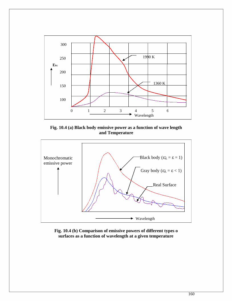
160

300

250 1990 K

Ebλ

200

150 1360 K

100

0 1 2 3 4 5 6

Wavelength

Fig. 10.4 (a) Black body emissive power as a function of wave length

and Temperature

Monochromatic Black body (ελ = ε = 1)

emissive power

Gray body (ελ = ε < 1)

Real Surface

Wavelength

Fig. 10.4 (b) Comparison of emissive powers of different types o surfaces as a function of wavelength at a given temperature

161

10.2.4 KIRCHOFF’S LAW:

This law states that the emissivity of a surface is equal to its absorptivity when the surface is in thermal equilibrium with the surroundings.

Proof: Consider a perfect black enclosure i.e. the one which absorbs all the incident radiation falling on it (see Fig 10.5). Now let the radiant flux from this enclosure per unit

area arriving at some area be qi W/m2.

Black Enclosure

EA

Sample

qi.A.α

Fig. 10.5 : Model used for deriving Kirchoff law

Now suppose that a body is placed inside the enclosure and allowed to come to thermal equilibrium with it. At equilibrium, the energy absorbed by the body must be equal to the

energy emitted; otherwise there would be an energy flow into or out of the body, which would raise or lower its temperature. At thermal equilibrium we may write

EA = qi A α ………………………………….(10.8)

If we now replace the body in the enclosure with a black body of the same size and shape

and allow it to come to thermal equilibrium with the enclosure,

EbA = qi A .......………………………………(10.9)

Since α = 1 for a blackbody.

If Eq. 10.8 is divided by Eq. 10.9 we get

E/Eb = α

But by definition E/Eb = ε, the emissivity of the body, so that ε = α…………(10.10)

162

Equation 10.10 is called Kirchoff‟s law and is valid only when the body is in thermal

equilibrium with the surroundings. However, while analyzing radiation problems in practice

we assume that Kirchoff‟s law holds good even if the body is not in thermal equilibrium with the surroundings, as the error involved is not very significant.

10.3 ILLUSTRATIVE EXAMPLES ON BASIC CONCEPTS

Example 10.1: The emission of radiation from a surface can be approximated as

blackbody radiation at 1000K.

(a) What fraction of the total energy emitted is below λ = 5μm (b) What is the wavelength below which the emission is 10.5% of the total emission at

1000K. (c) What is the wavelength at which the maximum spectral emission occurs at 1000K.

Solution: The radiation flux emitted by the blackbody over the wavelength interval 0 – λ

is given by

λ

[Eb]0 – λ = ∫Ebλdλ

0 The integration required in the above equation has been done numerically and the results

are presented in the form of a table. The table gives the value of D 0-λ where

λ

∫Ebλdλ 1 λ

D0-λ = 0 = ------- ∫ Ebλ dλ --- -∞-----------

∫Ebλdλ ζ T4 0

0

(a) From Table of Radiation properties, for λT = 5 x 1000 = 5000, D0-λ = 0.6337.

This means that 63.37 % of the total emission occurs below λ = 5 μm.

(b) From the same table, for D0-λ = 0.105, λT =

2222. Hence λ = 2222/1000 = 2.222 μm.

(c) From Wein‟s displacement law, λmT = 0.002898.

Hence for T = 1000 K, λm =0.002898 / 1000 = 2.898 x 10 −6

m = 2.898 μm.

Example 10.2: The monochromatic emissivity of a surface varies with the wavelength in

the following manner:

ελ = 0 for λ < 0.3μm = 0.9 for 0.3μm < λ < 1μm

= 0 for λ > 1μm Calculate the heat flux emitted by the surface if it is at a temperature of 1500 K

163

Solution: Eλ = ε λ Ebλ

∞ 0.3 μm 1 μm ∞

Therefore E = ∫ ε λ Ebλ = ∫ 0.0 Ebλ dλ + ∫ 0.9 Ebλ dλ + ∫ 0.0 Ebλ dλ 0 0 0.3 μm 1 μm

1 μm 1 μm 0.3 μm

= 0.9 ∫Ebλ dλ = 0.9 [ ∫ Ebλ dλ − ∫ Ebλ dλ ] 0.3 μm 0 0

= 0.9 ζ T 4 [ D0-1 – D0 – 0.3]

For λ = 1μm, λT = 1500 μm-K, therefore D0-1 = ½ (0.01972 + 0.00779) =

0.93755 For λ = 0.3μm, λT = 450 μm-K, therefore D0-3 = 0

Thus E = 0.9x5.67x10-8

x15004 [0.013755 – 0] = 3553 W/m

2

Example 10.3: Calculate the heat flux emitted due to thermal radiation from a black

surface at 60000 C. At what wavelength is the monochromatic emissive power maximum

and what is the maximum value?

Solution:Temp of the black surface = 6273K

Heat Flux emitted = Eb = ζT4 = 5.67x10

-8x6273

4 = 87798 KW/m

2

Wavelength corresponding to max monochromatic emissive power is given

by λmT = 0.002898 m-K

λm = 0.002898/6273 = 4.62x10-7

m

The maximum monochromatic emissive power is given by

2 π C1

(Ebλ)max = ------------------------------------

λmax [ exp {C2 / (λmaxT)} – 1]

2 x π x 0.596 x 10 − 16

= ---------------------------------------------------------------

(4.62 x 10 − 7

) 5 x [ exp{ 0.014387 / 0.002898} – 1]

= 1.251 x 10 14

W / m2

164

Example 10.4: The spectral hemispherical emissivity (monochromatic emissivity) of fire

brick at 750K as a function of wavelength is as follows:

ε1 = 0.1 for 0 < λ < 2μm

ε2 = 0.6 for 2μm < λ < 14μm

ε3 = 0.8 for14 < λ < ∞

Calculate the hemispherical emissivity, ε for all wavelengths.

Solution:

∞ E ∫ελ Ebλ dλ 1 λ1 λ2 λ3

ε = ------ = -0------------- = ------ [ ε1 ∫ Ebλ dλ + ε2 ∫ Ebλ dλ + ε3 ∫ Ebλ dλ ]

Eb ζ T 4 ζ T

4 0 λ1 λ2

Where λ1 = 2μm, λ2 = 14μm, λ3 = ∞

Thus = ε1D0-λ1 + ε2[D0-λ2 – D0-λ1] + ε3[D0-∞ – D0-λ2]

Now, λ1T = 2x750 = 1500; D0-λ1 = 0.013

λ2T = 14x750 = 10500; D0-λ2 = 0.924 λ3T = ∞; D0-λ3 = 1

Hence ε = 0.1 x 0.013 + 0.6 x [ 0.924 – 0.013] + 0.8 x [1 – 0.924] = 0.609

Example 10.5: the filament of a light bulb is assumed to emit radiation as a black body at 2400K. if the bulb glass has a transmissivity of 0.90 for radiation in the visible range,

calculate the percentage of the total energy emitted by the filament that reaches the ambient as visible light.

Solution: The wavelength range corresponding to the visible range is taken as

λ1 = 0.38μm to λ2 = 0.76μm. Therefore the fraction F of the total energy emitted in this range is given by

λ2

∫ Ebλ dλ λ2 λ1 F = η [

λ1--------- ] = η [ ∫Ebλ dλ − ∫Ebλ dλ ] / Eb

Eb (T) 0 0

= η [D0-λ2 – D0-λ1].

Now λ1T = 0.38 x 2400 = 912. Hence D0-λ1 = 0.0002

and λ2T = 0.76 x 2400 = 1824. Hence D0-λ2 = 0.0436

Therefore F = 0.9 x [0.0436 – 0.0002] =0.039 .

Only 3.9 % of the total energy enters the ambient as light. The remaining energy produces heating.

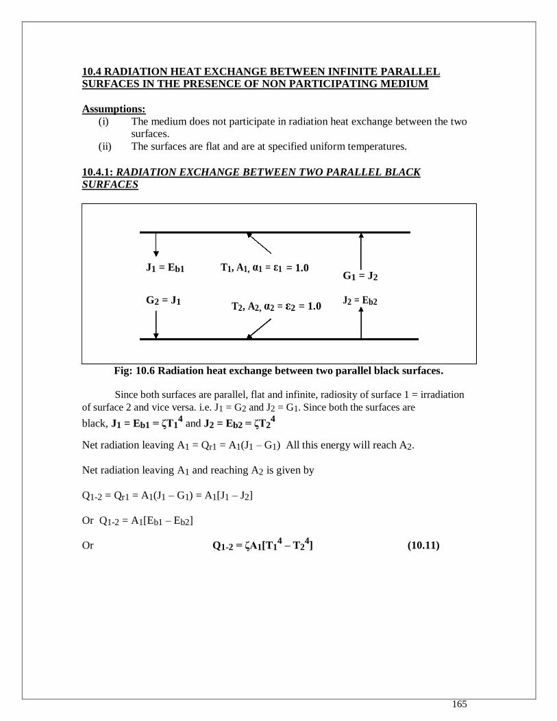
165

10.4 RADIATION HEAT EXCHANGE BETWEEN INFINITE PARALLEL

SURFACES IN THE PRESENCE OF NON PARTICIPATING MEDIUM

Assumptions: (i) The medium does not participate in radiation heat exchange between the two

surfaces. (ii) The surfaces are flat and are at specified uniform temperatures.

10.4.1: RADIATION EXCHANGE BETWEEN TWO PARALLEL BLACK

SURFACES

J1 = Eb1 T1, A1, α1 = ε1 = 1.0 G1 = J2

G2 = J1 T2, A2, α2 = ε2 = 1.0

J2 = Eb2

Fig: 10.6 Radiation heat exchange between two parallel black surfaces.

Since both surfaces are parallel, flat and infinite, radiosity of surface 1 = irradiation

of surface 2 and vice versa. i.e. J1 = G2 and J2 = G1. Since both the surfaces are

black, J1 = Eb1 = ζT14 and J2 = Eb2 = ζT2

4

Net radiation leaving A1 = Qr1 = A1(J1 – G1) All this energy will reach A2.

Net radiation leaving A1 and reaching A2 is given by

Q1-2 = Qr1 = A1(J1 – G1) = A1[J1 – J2]

Or Q1-2 = A1[Eb1 – Eb2]

Or Q1-2 = ζA1[T14 – T2

4] (10.11)

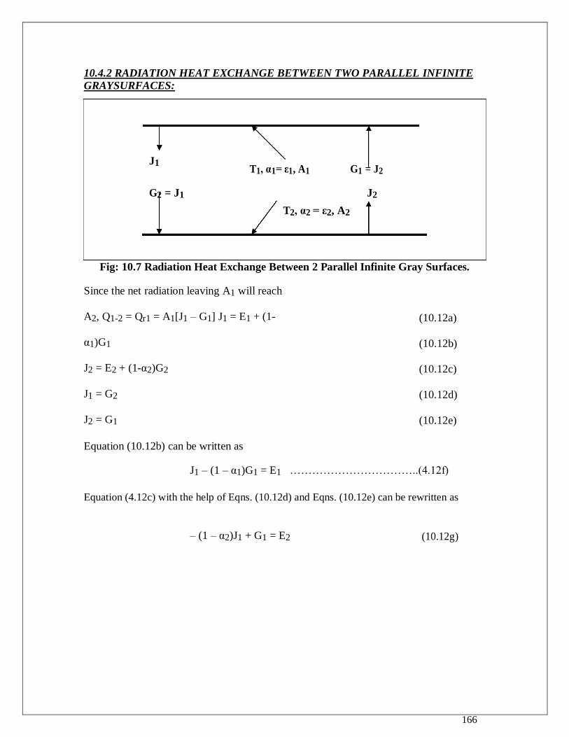
166

10.4.2 RADIATION HEAT EXCHANGE BETWEEN TWO PARALLEL INFINITE

GRAYSURFACES:

J1 T1, α1= ε1, A1 G1 = J2

G2 = J1

T2, α2

J2

= ε2, A2

Fig: 10.7 Radiation Heat Exchange Between 2 Parallel Infinite Gray Surfaces.

Since the net radiation leaving A1 will reach

A2, Q1-2 = Qr1 = A1[J1 – G1] J1 = E1 + (1-

α1)G1

J2 = E2 + (1-α2)G2

J1 = G2

J2 = G1

(10.12a)

(10.12b)

(10.12c)

(10.12d)

(10.12e)

Equation (10.12b) can be written as

J1 – (1 – α1)G1 = E1 ……………………………..(4.12f)

Equation (4.12c) with the help of Eqns. (10.12d) and Eqns. (10.12e) can be rewritten as

– (1 – α2)J1 + G1 = E2 (10.12g)

167

Solving for J1 and G1 from Eq. (10.12f) and (10.12g) we get

E1 + (1 – α1) E2

J1 = ----------------------------

1 – (1 – α1) (1 – α2)

ε1E b1 + (1 – α1) ε2E b2

Or J1 = ----------------------------- ……………………………..(10.13a)

1 – (1 – α1) (1 – α2)

ε2E b2 + (1 – α2) ε1E b1

and G1 = ----------------------------- ……………………………..(10.13b)

1 – (1 – α1) (1 – α2)

Substituting these expressions for J1 and G1 in Eq.( 10.12a) we get

A1

Q1-2 = -------------------------- [ε1E b1 + (1 – α1) ε2E b2 − ε2E b2 − (1 – α2) ε1E b1]

[1 – (1 – α1) (1 – α2)]

A1 [α2 ε1Eb1 − α1 ε2Eb2 ]

Or Q1-2 = ------------------------------------ [1 – (1 – α1) (1 – α2)]

Substituting for Eb1 and Eb2 in terms of temperatures we get

ζA1 [α2 ε1T14 − α1ε2T2

4]

Or Q1-2 = ------------------------------------ …………………………………….(10.14)

[1 – (1 – α1) (1 – α2)]

If Kirchoff‟s law holds good then α1 = ε1 and α2 = ε2.

ζA1 [ε1 ε2T14 − ε1ε2T2

4]

Hence Q1-2 = ------------------------------------

[1 – (1 – ε1) (1 – ε2)]

ζ A1 (T14 – T2

4)

Or Q1-2 = --------------------------- …………………………(10.15)

[ 1/ε1 + 1/ε2 − 1 ]

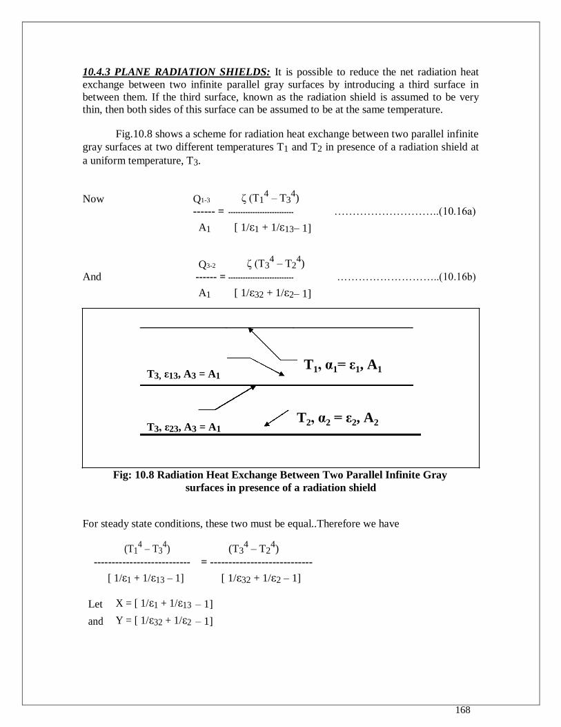
168

10.4.3 PLANE RADIATION SHIELDS: It is possible to reduce the net radiation heat

exchange between two infinite parallel gray surfaces by introducing a third surface in

between them. If the third surface, known as the radiation shield is assumed to be very thin, then both sides of this surface can be assumed to be at the same temperature.

Fig.10.8 shows a scheme for radiation heat exchange between two parallel infinite

gray surfaces at two different temperatures T1 and T2 in presence of a radiation shield at

a uniform temperature, T3.

Now Q1-3 ζ (T14 – T3

4)

------ = --------------------------- ………………………..(10.16a)

A1 [ 1/ε1 + 1/ε13 – 1]

Q3-2 ζ (T34 – T2

4)

And ------ = --------------------------- ………………………..(10.16b)

A1 [ 1/ε32 + 1/ε2 – 1]

T3, ε13, A3 = A1 T1, α1= ε1, A1

T3, ε23, A3 = A1 T2, α2 = ε2, A2

Fig: 10.8 Radiation Heat Exchange Between Two Parallel Infinite Gray surfaces in presence of a radiation shield

For steady state conditions, these two must be equal..Therefore we have

(T14 – T3

4) (T3

4 – T2

4)

--------------------------- = ----------------------------

[ 1/ε1 + 1/ε13 – 1] [ 1/ε32 + 1/ε2 – 1]

Let X = [ 1/ε1 + 1/ε13 – 1]

and Y = [ 1/ε32 + 1/ε2 – 1]

169

Then,

(T14 – T3

4) (T3

4 – T2

4)

--------------- = ------------------

X Y

Solving for T3 we get

-----------------------------T14+(X/Y)T24

] 1 / 4

…………………(10.16c)

T3 = [

(1 + X /Y)

Substituting this value of T3 in Eq. (10.16a) we get

Q1-3 / A1 = Q3-2 / A1 = (Q1-2 / A)1 Rad.Shield = ζ { T2 4 – [{T1

4 +(X/Y)T2

4}/(1 + X/Y)] } / X

…………………….(10.17a)

Special case:

When ε1 = ε2 = ε13 = ε32 = ε, then X = Y = (2/ε) − 1

Hence, T3 = [(T1 4+ T2

4) / 2 ]

¼………………………..(10.18a)

ζ{ T14 − [(T1

4 + T2

4) / 2 ]

and [Q1-2 / A ]1 rad shield = -------------------------------------

[2/ε − 1]

ζ [T14 − T2

4]

= ------------------------ ………………………………(10.18b)

2 [2/ε − 1]

It can be seen from the above equation that when the emissivities of all surfaces are equal, the net radiation heat exchange between the surfaces in the presence of single

radiation shield is 50% of the radiation heat exchange between the same two surfaces

without the presence of a radiation shield. This statement can be generalised for N

radiation shields as follows: 1

[Q1-2 / A]N shields = --------- [Q1-2 / A] without shield ……………(10.18c)

(N + 1)

170

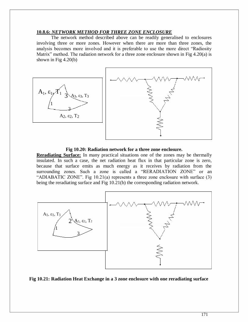
171

10.8.6: NETWORK METHOD FOR THREE ZONE ENCLOSURE

The network method described above can be readily generalised to enclosures

involving three or more zones. However when there are more than three zones, the

analysis becomes more involved and it is preferable to use the more direct “Radiosity

Matrix” method. The radiation network for a three zone enclosure shown in Fig 4.20(a) is shown in Fig 4.20(b)

A1, ε1, T1 3 A3, ε3, T3

1

2

A2, ε2, T2

Fig 10.20: Radiation network for a three zone enclosure.

Reradiating Surface: In many practical situations one of the zones may be thermally

insulated. In such a case, the net radiation heat flux in that particular zone is zero,

because that surface emits as much energy as it receives by radiation from the

surrounding zones. Such a zone is called a “RERADIATION ZONE” or an

“ADIABATIC ZONE”. Fig 10.21(a) represents a three zone enclosure with surface (3) being the reradiating surface and Fig 10.21(b) the corresponding radiation network.

A1, ε1, T1

2 A2, ε2, T2

1

3

Fig 10.21: Radiation Heat Exchange in a 3 zone enclosure with one reradiating surface

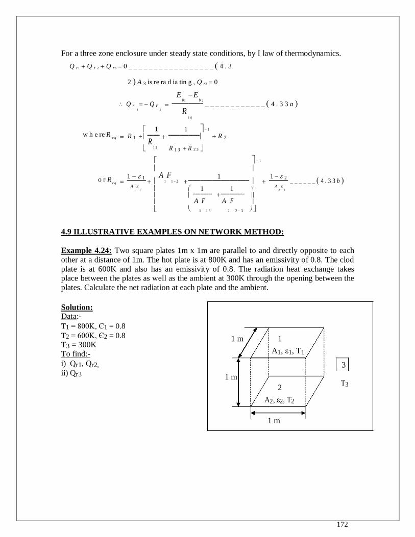
172

For a three zone enclosure under steady state conditions, by I law of thermodynamics.

Q r1 Q r 2 Q r3 0 _ _ _ _ _ _ _ _ _ _ _ _ _ _ _ _ _ 4 . 3

2 A 3 is re ra d ia tin g , Q r3 0

w h e re R

o r R

e q e q

Q r Q r

E b1

E

b 2 _ _ _ _ _ _ _ _ _ _ _ _ 4 . 3 3 a

1 2 R e q

R 1 1

1 1 R 2

R 1 2

R 1 3 R

2 3

1

1 1

1

1 2

A

1

F1 2

_ _ _ _ _ _ 4 . 3 3 b

A 1

1 1

1 A

2

2

A F

A

F

1 3

2 2 3

1

4.9 ILLUSTRATIVE EXAMPLES ON NETWORK METHOD:

Example 4.24: Two square plates 1m x 1m are parallel to and directly opposite to each

other at a distance of 1m. The hot plate is at 800K and has an emissivity of 0.8. The clod

plate is at 600K and also has an emissivity of 0.8. The radiation heat exchange takes place between the plates as well as the ambient at 300K through the opening between the

plates. Calculate the net radiation at each plate and the ambient.

Solution:

Data:-

T1 = 800K, Є1 = 0.8

T2 = 600K, Є2 = 0.8

T3 = 300K

To find:-

i) Qr1, Qr2,

ii) Qr3

1 m 1

A1, ε1, T1

3

1 m

T3

2

A2, ε2, T2

1 m

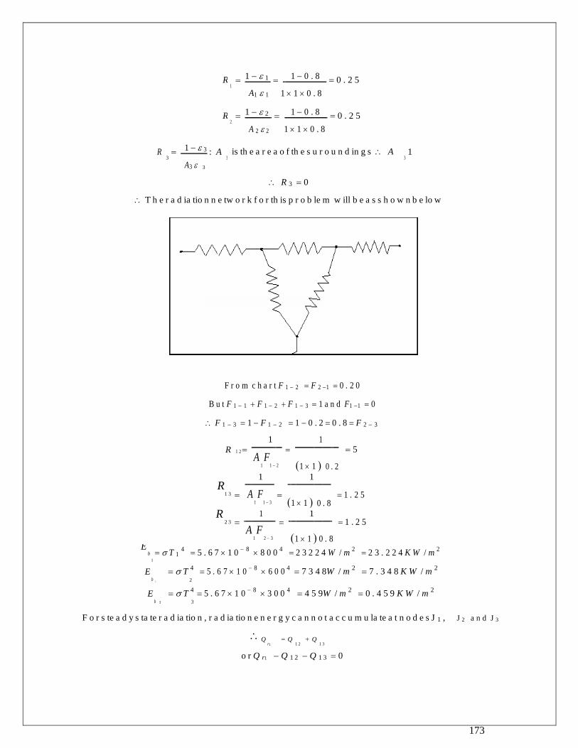
173

R 1 1 1 0 . 8 0 . 2 5

1

A1 1

1 1 0 . 8

R 1 2 1 0 . 8

0 . 2 5

2

A 2 2

1 1 0 . 8

R 1 3 : A is th e a r e a o f th e s u r o u n d in g s A 1

3

3 3

A3

3

R 3 0

T h e r a d ia tio n n e tw o r k f o r th is p r o b le m w ill b e a s s h o w n b e lo w

F r o m c h a r t F 1 2 F 2 1 0 . 2 0

B u t F 1 1 F 1 2 F 1 3 1 a n d F1 1 0

F 1 3 1 F 1 2 1 0 . 2 0 . 8 F 2 3

R

1

1 5

1 2 A

1

F1 2

1 1 0 . 2

R1 3

1

1

1 . 2 5

A 1

F1 3

1 1 0 . 8

R 2 3

1

1 1 . 2 5

A 1

F 2 3

1 1 0 . 8

E b T 1

4 5 . 6 7 1 0

8 8 0 0

4 2 3 2 2 4 W / m

2 2 3 . 2 2 4 K W / m

2

1

E b T

4 5 . 6 7 1 0 8 6 0 0

4 7 3 4 8W / m 2 7 . 3 4 8 K W / m

2

2 2

E b T

4 5 . 6 7 1 0 8 3 0 0

4 4 5 9W / m 2 0 . 4 5 9 K W / m

2

3 3

F o r s te a d y s ta te r a d ia tio n , r a d ia tio n e n e r g y c a n n o t a c c u m u la te a t n o d e s J 1 , J 2 a n d J 3

Q

r1 Q 1 2 Q 1 3

o r Q r1 Q 1 2 Q 1 3 0

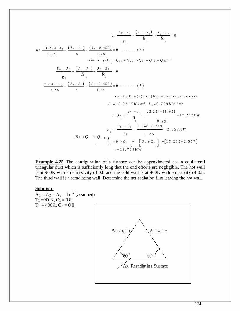
174

E b J 1 J

1 J 2

J

1 J 3 0

1

R 1

R 1 2

R1 3

o r 2 3 . 2 2 4 J 1

J 1 J 2

J 1 0 . 4 5 9

0 _ _ _ _ _ _ _ a

0 . 2 5 5 1 . 2 5

s im ila r ly Q r 2 Q 2 1 Q 2 3 Q r Q 2 1 Q 2 3 0

2

E b 2 J 2

J

2 J 1

J 2 E b

3 0

R 2

R 1 2

R 2 3

7 . 3 4 8 J 2 J 2 J 1

J 2 0 . 4 5 9

0 _ _ _ _ _ _ _ b

0 . 2 5 5 1 . 2 5

J 1

Q

r2

B u t Q Q

Q r1 r 2 r3

S o lv in g E q n ( a ) a n d ( b ) s im u lta n e o u s ly w e g e t

1 8 . 9 2 1 K W / m 2 ; J

2 6 . 7 0 9 K W / m 2

Q r E b J 1

2 3 . 2 2 4 1 8 . 9 2 1

1 7 . 2 1 2 K W

1

R1

0 . 2 5

1

E b J 2

7 . 3 4 8 6 . 7 0 9

2 . 5 5 7 K W

2

R 2

0 . 2 5

0 Q r Q r Q r 1 7 . 2 1 2 2 . 5 5 7

3 1 2

1 9 . 7 6 9 K W

Example 4.25 The configuration of a furnace can be approximated as an equilateral triangular duct which is sufficiently long that the end efforts are negligible. The hot wall

is at 900K with an emissivity of 0.8 and the cold wall is at 400K with emissivity of 0.8.

The third wall is a reradiating wall. Determine the net radiation flux leaving the hot wall.

Solution:

A1 = A2 = A3 = 1m2 (assumed)

T1 =900K, Є1 = 0.8

T2 = 400K, Є2 = 0.8

A1, ε1, T1 A2, ε2, T2

600

600

A3, Reradiating Surface

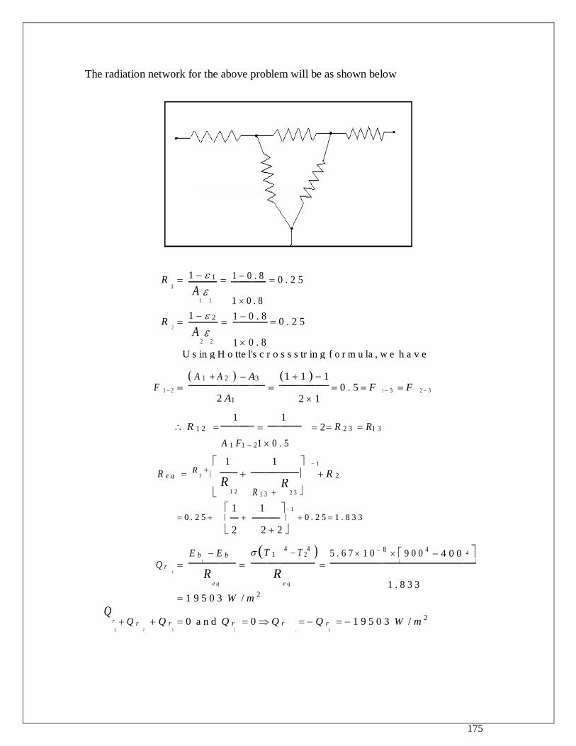
175

The radiation network for the above problem will be as shown below

R 1 1 1 0 . 8 0 . 2 5

1

A1

1

1

0 . 8

R

1 2

1 0 . 8 0 . 2 5

2

A 2

2

0 . 8

1

U s in g H o tte l's c r o s s s tr in g f o r m u la , w e h a v e

A 1 A 2 A3 1 1 1

F 1 2

0 . 5 F 1 3 F 2 3

2 A1

2 1

R 1 2

1

1 2 R 2 3 R1 3

A 1 F1 21 0 . 5

1 1 1

R e q R 1

R 2

R 1 2

R 1 3

R

2 3

1 1 1

0 . 2 5 0 . 2 5 1 . 8 3 3

2 2 2

E b E b 2 T 1

4 T 2

4 5 . 6 7 1 0

8 9 0 0

4 4 0 0 4

Q r 1

R e q

R e q

1 . 8 3 3

1

1 9 5 0 3 W / m 2

Q r Q r

2 Q r 0 a n d Q r 0 Q r Q r 1 9 5 0 3 W / m

2

1 3 3 2 1

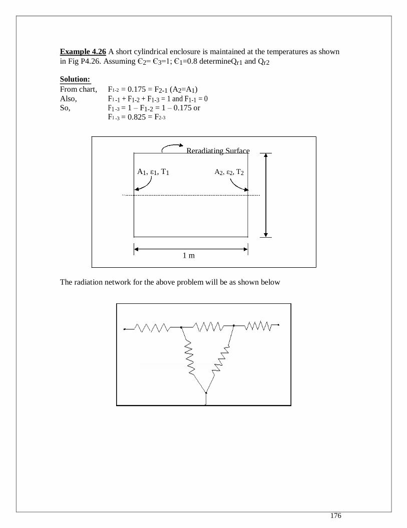
176

Example 4.26 A short cylindrical enclosure is maintained at the temperatures as shown

in Fig P4.26. Assuming Є2= Є3=1; Є1=0.8 determineQr1 and Qr2

Solution:

From chart, F1-2 = 0.175 = F2-1 (A2=A1)

Also, F1 -1 + F1-2 + F1-3 = 1 and F1-1 = 0

So, F1 -3 = 1 – F1-2 = 1 – 0.175 or F1 -3 = 0.825 = F2-3

Reradiating Surface

A1, ε1, T1 A2, ε2, T2

1 m

The radiation network for the above problem will be as shown below

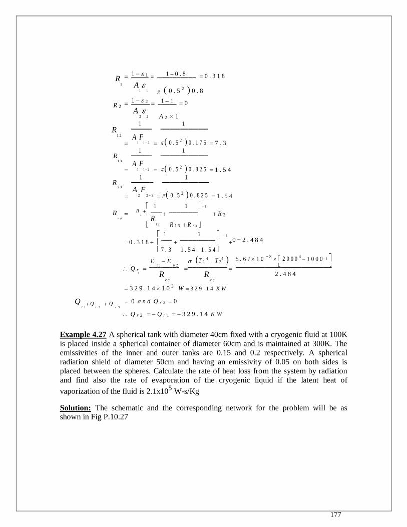
177

R1

R 2

R1 2

R1 3

R 2 3

R e q

Q r 1 Qr2Qr3

1 1 1 0 . 8 0 . 3 1 8

A

1

1 0 . 5 2 0 . 8

1 2 1 1 0

A

2

2 A 2 1

1

1

7 . 3

A 1

F1 2 0 . 5 2 0 . 1 7 5

1

1

1 . 5 4

A 1

F1 2 0 . 5 2 0 . 8 2 5

1

1

1 . 5 4

A 2

F 2 3 0 . 5 2 0 . 8 2 5

1 1 1

R

1

R 2

R 1 2

R 1 3 R

2 3

1 1 1

0 . 3 1 8

7 . 3 1 . 5 4 1 . 5 4

E b 1 E

b 2 T 1 4 T 2

4

Q r

R e q

R e q

1

3 2 9 . 1 4 1 0 3 W 3 2 9 . 1 4K W 0 a n d Q r 3 0 Q r 2 Q r 1 3 2 9 . 1 4 K W

0 2 . 4 8 4

5 . 6 7 1 0 8 2 0 0 0 4 1 0 0 0 4

2 . 4 8 4

Example 4.27 A spherical tank with diameter 40cm fixed with a cryogenic fluid at 100K

is placed inside a spherical container of diameter 60cm and is maintained at 300K. The

emissivities of the inner and outer tanks are 0.15 and 0.2 respectively. A spherical

radiation shield of diameter 50cm and having an emissivity of 0.05 on both sides is

placed between the spheres. Calculate the rate of heat loss from the system by radiation

and find also the rate of evaporation of the cryogenic liquid if the latent heat of

vaporization of the fluid is 2.1x105 W-s/Kg

Solution: The schematic and the corresponding network for the problem will be as

shown in Fig P.10.27

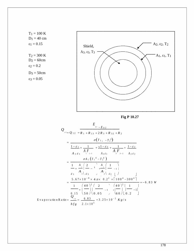
178

T1 = 100 K

D1 = 40 cm

ε1 = 0.15 Shield,

A2, ε2, T2

T2 = 300 K A3, ε3, T3

A1, ε1, T1

D2 = 60cm

ε2 = 0.2

D3 = 50cm

ε3 = 0.05

Fig P 10.27

Q r 1 Q 1 2

E

b 1 E b 2

R 1 R 1 3 2 R 3 R 3 2 R 2

T 1 4 T 24

1

2 1 3

1

1 2

1 1

A 1 1 A

1

F 1 3 A 3 3

A 3

F 3 2 A 2 2

A 1 T 1 4 T 2

4

A

A

1 1 2

1 1

1

1

1

3

2

A

3 A

2

5 . 6 7 1 0 8

4 0 . 2 2 1 0 0 4 3 0 0 4 6 . 8 3 W

4 0 2

4 0 2

1 2 1

1

1

0 . 1 5

5 0 0 . 0 5 6 0 0 . 2

E v a p o r a tio n R a tio Q

r 1 6 . 8 3 3 . 2 5 1 0 5 K g / s

h f g 2 . 1 1 0 5