LECTURE NOTES FOR THE COURSE - UCLA Department …biskup/275a.1.17f/PDFs/245A-notes.pdf · LECTURE NOTES FOR THE COURSE ... Frostman’s lemma ... The lemma is proved by ...

LECTURE NOTES FOR THE COURSE

MATH 245A: GRADUATE ANALYSIS

FALL QUARTER 2014

BY MAREK BISKUP

Note: Preliminary version, comments welcome!

0

CONTENTS

1. A brief history of integral . . . . . . . . . . . . . . . . . . . . . . . . . . . . . . . . . . . . . . . . . . . . . . . . . . . . . . . 11.1. Newton’s integral . . . . . . . . . . . . . . . . . . . . . . . . . . . . . . . . . . . . . . . . . . . . . . . . . . . . . . . . . . 11.2. Cauchy’s integral . . . . . . . . . . . . . . . . . . . . . . . . . . . . . . . . . . . . . . . . . . . . . . . . . . . . . . . . . . 21.3. Riemann’s integral . . . . . . . . . . . . . . . . . . . . . . . . . . . . . . . . . . . . . . . . . . . . . . . . . . . . . . . . . 31.4. Stieltjes’ integral . . . . . . . . . . . . . . . . . . . . . . . . . . . . . . . . . . . . . . . . . . . . . . . . . . . . . . . . . . . 51.5. Stieltjes and beyond: Ito-Stratonovich and Young integrals . . . . . . . . . . . . . . . . . . . . . 7

2. Peano-Jordan content . . . . . . . . . . . . . . . . . . . . . . . . . . . . . . . . . . . . . . . . . . . . . . . . . . . . . . . . . . . 102.1. Elementary sets and (pre)content . . . . . . . . . . . . . . . . . . . . . . . . . . . . . . . . . . . . . . . . . . . . 102.2. Outer/inner content, measurability . . . . . . . . . . . . . . . . . . . . . . . . . . . . . . . . . . . . . . . . . . . 132.3. Non-measurable sets, relation to topology . . . . . . . . . . . . . . . . . . . . . . . . . . . . . . . . . . . . 172.4. Connection with Riemann integral . . . . . . . . . . . . . . . . . . . . . . . . . . . . . . . . . . . . . . . . . . . 18

3. Lebesgue measure . . . . . . . . . . . . . . . . . . . . . . . . . . . . . . . . . . . . . . . . . . . . . . . . . . . . . . . . . . . . . . 203.1. Lebesgue outer measure . . . . . . . . . . . . . . . . . . . . . . . . . . . . . . . . . . . . . . . . . . . . . . . . . . . . 203.2. Lebesgue measurable sets . . . . . . . . . . . . . . . . . . . . . . . . . . . . . . . . . . . . . . . . . . . . . . . . . . . 243.3. Lebesgue measure . . . . . . . . . . . . . . . . . . . . . . . . . . . . . . . . . . . . . . . . . . . . . . . . . . . . . . . . . . 273.4. Convergence Theorems . . . . . . . . . . . . . . . . . . . . . . . . . . . . . . . . . . . . . . . . . . . . . . . . . . . . . 293.5. Nonmeasurable sets . . . . . . . . . . . . . . . . . . . . . . . . . . . . . . . . . . . . . . . . . . . . . . . . . . . . . . . . 31

4. Lebesgue integral: bounded case . . . . . . . . . . . . . . . . . . . . . . . . . . . . . . . . . . . . . . . . . . . . . . . . . 334.1. Bounded functions on finite measure spaces . . . . . . . . . . . . . . . . . . . . . . . . . . . . . . . . . . 334.2. Integrability vs measurability . . . . . . . . . . . . . . . . . . . . . . . . . . . . . . . . . . . . . . . . . . . . . . . . 374.3. Bounded Convergence Theorem . . . . . . . . . . . . . . . . . . . . . . . . . . . . . . . . . . . . . . . . . . . . . 414.4. Characterization of Riemann integrability . . . . . . . . . . . . . . . . . . . . . . . . . . . . . . . . . . . . . 43

5. Lebesgue integral: general case . . . . . . . . . . . . . . . . . . . . . . . . . . . . . . . . . . . . . . . . . . . . . . . . . . 475.1. Unsigned integral . . . . . . . . . . . . . . . . . . . . . . . . . . . . . . . . . . . . . . . . . . . . . . . . . . . . . . . . . . 475.2. Signed integral and convergence theorems . . . . . . . . . . . . . . . . . . . . . . . . . . . . . . . . . . . . 505.3. Absolute integrability and L1-space . . . . . . . . . . . . . . . . . . . . . . . . . . . . . . . . . . . . . . . . . . 535.4. Uniform integrability . . . . . . . . . . . . . . . . . . . . . . . . . . . . . . . . . . . . . . . . . . . . . . . . . . . . . . . 55

6. Abstract measure theory . . . . . . . . . . . . . . . . . . . . . . . . . . . . . . . . . . . . . . . . . . . . . . . . . . . . . . . . 596.1. From semialgebras to outer measures . . . . . . . . . . . . . . . . . . . . . . . . . . . . . . . . . . . . . . . . 596.2. Caratheodory measurability and extension theorem . . . . . . . . . . . . . . . . . . . . . . . . . . . . 626.3. Uniqueness of extension . . . . . . . . . . . . . . . . . . . . . . . . . . . . . . . . . . . . . . . . . . . . . . . . . . . . 666.4. Lebesgue-Stieltjes measures . . . . . . . . . . . . . . . . . . . . . . . . . . . . . . . . . . . . . . . . . . . . . . . . . 69

7. More on outer measures . . . . . . . . . . . . . . . . . . . . . . . . . . . . . . . . . . . . . . . . . . . . . . . . . . . . . . . . . 737.1. Regular outer measures . . . . . . . . . . . . . . . . . . . . . . . . . . . . . . . . . . . . . . . . . . . . . . . . . . . . . 737.2. Borel regular and Radon measures . . . . . . . . . . . . . . . . . . . . . . . . . . . . . . . . . . . . . . . . . . . 757.3. Metric outer measures . . . . . . . . . . . . . . . . . . . . . . . . . . . . . . . . . . . . . . . . . . . . . . . . . . . . . . 777.4. Hausdorff measure and dimension . . . . . . . . . . . . . . . . . . . . . . . . . . . . . . . . . . . . . . . . . . . 807.5. Frostman’s lemma. . . . . . . . . . . . . . . . . . . . . . . . . . . . . . . . . . . . . . . . . . . . . . . . . . . . . . . . . . 85

245A lecture notes ( c©2017 M. Biskup) Preliminary version (typeset: September 22, 2017)

1

1. A BRIEF HISTORY OF INTEGRAL

The MATH 245A analysis course is by and large devoted to Lebesgue’s theory of measure andintegration. This theory stands on the foundations laid over 200 years by many great mindsworking in mathematics. In order to appreciate these better, we begin by a brief recount of thehistory of integral and the rather winding road that led to Lebesgue’s ultimate formulation.

In what follows, I will freely invoke various technical terms such as limit, continuity, deriva-tive, etc, pertinent to differential calculus. These are introduced and discussed in detail in variousundergraduate analysis courses (e.g., MATH 131).

1.1 Newton’s integral.

At the time of Newton (and Leibnitz), integral was understood in the sense of an “inverse” toderivative. The interpretation in terms of “area under graph of function” was known but wasregarded as secondary. We may thus take Newton’s definition of integral to be:

Definition 1.1 (Newton’s integral) Let f : [a,b]→ R and let F be such that F ′(x) = f (x) for allx ∈ [a,b]. Then ∫ b

af (x)dx := F(b)−F(a) (1.1)

Newton’s integral thus required the function to have an antiderivative (a.k.a. the primitive func-tion). The definition needs to be supplied by the following observation that, we note, uses onlydifferential calculus:

Lemma 1.2 If F : [a,b]→ R is such that F ′(x) = 0 for all x ∈ [a,b], then F is constant.

Indeed, if there are two antiderivatives for f (x), then their difference has zero derivative andso must be constant. The lemma is proved by way of:

Theorem 1.3 (Mean-Value Theorem) Let f : [a,b]→ R be continuous on [a,b] and such thatf ′(x) exists for all x ∈ (a,b). Then there is c ∈ (a,b) such that

f (b)− f (a)b−a

= f ′(c). (1.2)

It is worth noting that, since we require no regularity of f ′, the Mean-Value Theorem re-quires some facts from point-set topology that were certainly not available at the time of New-ton. Indeed, a linear transformation reduces the statement to the case f (b) = f (a), which goesby the name Rolles’ Theorem. This is in turn proved by using that a continuous function ona compact interval achieves its maximum and minimum in the interior for which we need theBolzano-Weierstrass Theorem (stating that every bounded sequence of reals has a convergingsubsequence). A simple argument underlying the first-derivative criterion then gives the result.

An attractive feature of Newton’s definition is that, once the integral is well defined, we imme-diately get both basic formulations of the Fundamental Theorem of Calculus:

Fundamental Theorem of Calculus I: The derivative of the integral with respect to the upperlimit is the integrand,

ddx

∫ x

af (t)dt = f (x) (1.3)


2

Fundamental Theorem of Calculus II: The integral of the derivative of a function equals thefunction itself, ∫ x

aF ′(t)dt = F(x) (1.4)

A major shortcoming of Newton’s integral is that its definition is non-constructive. In particu-lar, there is no direct way to decide whether a given function admit antiderivatives. This is, in asense, the key issue in all definitions that followed Newton’s.

1.2 Cauchy’s integral.

In his 1821 monograph, Cauchy put forward a definition of integral that is directly based on theinterpretation of “area under graph of function.” To state this precisely, we need some notation.(For the impatient, this notation will carry through a bunch of forthcoming subsections.) Given aninterval [a,b], a marked partition Π of an interval [a,b] is a collection of intervals {[xi−1,xi) : i =1, . . . ,n} and points z1, . . . ,zn such that

a = x0 < x1 < · · ·< xn−1 < xn = b (1.5)

andzi ∈ [xi−1,xi], i = 1, . . . ,n. (1.6)

The norm of the partition Π is defined by

‖Π‖ := maxi=1,...,n

|xi− xi−1|. (1.7)

Given a function f : [a,b]→ R and a marked partition Π of [a,b], we then define

R( f ,Π) :=n

∑i=1

f (zi)(xi− xi−1). (1.8)

(Here “R” is for Riemann sum.) Cauchy then more or less proved:

Theorem 1.4 (Cauchy’s integral) Let f : [a,b]→ R be continuous. Then the limit∫ b

af (x)dx := lim

‖Π‖→0R( f ,Π) (1.9)

exists (finitely) in the sense that

limδ↓0

infΠ : ‖Π‖<δ

R( f ,Π) = limδ↓0

supΠ : ‖Π‖<δ

R( f ,Π) (1.10)

where the supremum/infimum is over marked partitions Π of [a,b].

For the proof, it suffices to note that since f is continuous, it is in fact uniformly continuous(again by the aforementioned Bolzano-Weierstrass Theorem). Explicitly, given any ε > 0 thereis δ > 0 such that

x,y ∈ [a,b] & |x− y|< δ ⇒∣∣ f (y)− f (x)

∣∣< ε. (1.11)

It follows that, if Π and Π′ are two marked partitions with same x1, . . . ,xn but (possibly) differentz1, . . . ,zn, ∣∣R( f ,Π)−R( f ,Π′)

∣∣≤∑i=1

∣∣ f (zi)− f (z′i)∣∣(xi− xi−1)< ε(b−a). (1.12)


3

The right-hand side tends to zero as ε ↓ 0 and so the choice of the marked points thus playsno role for the limit and so we may as well choose one that makes R( f ,Π) maximal. Thiscorresponds to zi being the maximizer of f over [xi−1,xi]. But for such partition the limit existsby monotonicity because refining the partition decreases (maximal) R( f ,Π). (We will discussthis more in the context of upper and lower integrals in the next subsection.)

Cauchy completed his theory by providing proofs of both versions of the Fundamental Theo-rem of Calculus. Thanks to him, there was a first constructive definition of the definite integralfor which the classic Newton-Leibnitz theory applied. It seemed that harmony was achieved;unfortunately, not for too long.

1.3 Riemann’s integral.

The first half of the 19th century was marked by gradual but steady increase in precision withwhich mathematicians approached various questions surrounding the theory of functions. Ini-tially, there was not even a consensus about what it meant for a function to be continuous —before Cauchy, continuity meant that the same expression defining f (x) applied to the entire do-main of allowed x values. Numerous examples of discontinuous functions (in present-day senseof the word) were being considered and argued about. This permitted to extend Cauchy’s defi-nition to even functions with a finite number of points of discontinuity, in fact, even such pointswhere the integrand is unbounded.

For instance, when f : [a,c)∪ (c,b]→ R is given with f continuous on both [a,c) and (c,b],we may define ∫ b

af (x)dx := lim

ε,ε ′↓0

(∫ c−ε

af (x)dx+

∫ b

c+ε ′f (x)dx

), (1.13)

provided the double limit exists. The resulting object is referred to as an improper integral. (It iseasy to check that, if f is in fact continuous on all of [a,b], then this coincides with the originalnotion.) There are even more stringent recipes, e.g., given a < 0 < b we set

PV∫ b

a

1x

dx := limε↓0

(∫ −ε

a

1x

dx+∫ b

ε

1x

dx)

(1.14)

where “PV” stands for principal value. (It is easy to check that the integral of 1x fails to exists as

an improper integral, yet it does exists in the sense of principal value.) Notwithstanding, all ofthese attempts carry additional choices that make the concept difficult to use. In particular, thereare properties that naturally hold for the ordinary integral but fail for these extensions.

In his habilitation work, Riemann made a significant philosophical leap compared to all earlierattempts. Here is the definition he used:

Definition 1.5 (Riemann’s integral) Given f : [a,b] → R, we say that the Riemann integral∫ ba f (x)dx exists if the limit ∫ b

af (x)dx := lim

‖Π‖→0R( f ,Π), (1.15)

defined in the sense of equality (1.10), exists (finitely). The function f is then said to be Riemannintegrable on [a,b].


4

The most notable fact is that the existence of an integral is no longer derived from assumptionson regularity of f ; instead, it becomes a regularity property itself. To make the work with hisconcept easier, Riemann supplied a condition for f to be integrable in his sense:

Lemma 1.6 A function f : [a,b]→ R is Riemann integrable on [a,b] if and only if

lim‖Π‖→0

n

∑i=1

osc(

f , [xi−1,xi])(xi− xi−1) = 0. (1.16)

Here osc(

f ,A) is the oscillation of f on set A which is defined by

osc(

f ,A) := sup{| f (y)− f (x)| : x,y ∈ A

}(1.17)

and the limit is over partitions of [a,b] without marked points.

We leave the proof of this fact to homework. Note that this criterion shows almost instantlythat all continuous f are Riemann integrable. Riemann’s definition thus subsumes Cauchy’scompletely. We will later see this does not quite apply to Newton’s definition.

Another way how to define the integral is by way already touched upon in the section onCauchy’s integral. This method is generally attributed to Darboux — and, in the French literature,Darboux’s name is occasionaly used instead of Riemann’s in connection with this integral —although there are certainly predecessors to this. The idea is to introduce the upper Darboux sum,

U( f ,Π) :=n

∑i=1

(sup

t∈[xi−1,xi]

f (t))(xi− xi−1) (1.18)

and the lower Darboux sum,

L( f ,Π) :=n

∑i=1

(inf

t∈[xi−1,xi]f (t))(xi− xi−1). (1.19)

These sums now depend only on the partition Π; no additional marked points are necessary. Anencouraging feature of these is the behavior under refinements of the partition. Indeed, considera partition Π′ obtained by inserting a point (or points) into Π. Then

U( f ,Π)≥U( f ,Π′) while L( f ,Π)≤ L( f ,Π′). (1.20)

It follows that the limit ‖Π‖ → 0 can be simulated by taking infimum, resp., supremum of thesequantities. This leads to the definition of upper and lower Riemann/Darboux integrals,∫ b

af (x)dx := sup

Π

L( f ,Π) and∫ b

af (x)dx := inf

ΠU( f ,Π). (1.21)

A key point to note is then:

Lemma 1.7 f : [a,b]→ R is Riemann integrable on [a,b] if and only if∫ b

af (x)dx =

∫ b

af (x)dx (1.22)

The common value of these integrals then coincides with∫ b

a f (x)dx.


5

Given its generality, it is no surprise that Riemann’s definition includes functions that hadheretofore seemed inaccessible. To give an example, pick a non-increasing sequence {αn} withan ≥ 0 and consider an enumeration of rationals into a sequence, Q= {qi : i≥ 1}. Define

f (x) :=

{αn, if x = qn for some n≥ 1,0, otherwise.

(1.23)

Since {αn} is non-increasing, osc(

f , [xi−1,xi])> αn only for at most n intervals in the partition.

Hence, the sum in (1.16) is less than nαn+αn(b−a). Thus, if nαn→ 0, this function is Riemannintegrable. But once an > 0 for all n, this function is also discontinuous at all rationals! Moreover,it is not hard to check that ∫ b

af (x)dx = 0 (1.24)

for all a < b. In particular, the Fundamental Theorem of Calculus I fails at rational x.The previous example shows that Riemann’s integral is strictly more general than Cauchy’s.

To see that it does not even subsume Newton’s integral, we state:

Lemma 1.8 (Volterra’s example) There exists a function F : [a,b]→ R with F ′(x) defined andbounded at all x ∈ [a,b] and yet F ′ not Riemann integrable on [a,b].

Thus, although Riemann’s definition of integral is more general than Cauchy’s, it is perhapstoo general to make the FTC I work at all points and yet not general enough to make the FTC IIwork. This is a quandary that only Lebegue’s notion of measurable function (and identificationof those functions that differ on a set of measure zero) was able to resolve.

There are numerous other shortcomings of the Riemann integral that complicate its use. Wename just a few:

(1) The integral requires the integrated function to be bounded.(2) The integral behaves poorly under pointwise limits: There is a sequence of continuous

functions converging pointwise to a bounded function that is not Riemann integrable.

Further shortcomings concern generalizations of the Riemann integral to higher dimensions whichshould be quite obvious: Partition integration domain into squares and take a limit of the corre-sponding Riemann sum. Notwithstanding, we then run into:

(3) Generalizations to two (or higher) dimensions require additional conditions on the under-lying domain of integration. Or, taking this problem back to one dimension, the integralis defined more or less only for intervals.

(4) Fubini’s theorem, stating that an integral over a rectangle in R2 can be computed astwo successive one-dimensional integrals requires unwieldy conditions. Indeed, even iff : R2→ R is Riemann integrable, g(x) := f (x,y) may not be.

Again, all of these are resolved very elegantly in Lebesgue’s theory.

1.4 Stieltjes’ integral.

Before we move to discussing Lebesgue’s theory, it is worth pointing out a generalization ofRiemann’ integral, due to Stieltjes. This involves two functions, f ,g : [a,b]→ R for which we


6

consider the sum

S( f ,dg,Π) :=n

∑i=1

f (zi)(g(xi)−g(xi−1)

). (1.25)

Obviously, when g(x) := x, this degenerates to R( f ,Π).

Definition 1.9 (Stieltjes’ integral) A function f is said to be Riemann-Stieltjes integrable withrespect to g on [a,b] if ∫ b

af dg := lim

‖Π‖→0S( f ,dg,Π) (1.26)

exists (in the above sense). The resulting value defines the Riemann-Stieltjes integral.

We note that, although the Stieltjes integral appears quite asymmetric in f and g, there isactually a lot of symmetry. In fact, we have:

Lemma 1.10 If∫ b

a f dg exists, then so does∫ b

a gd f and∫ b

af dg+

∫ b

agd f = f (b)g(b)− f (a)g(a). (1.27)

Note that this boils down to the integration by parts formula when f and g are continuouslydifferentiable. Indeed, we have:

Lemma 1.11 If g is continuously differentiable,∫ b

af dg =

∫ b

af (x)g′(x)dx (1.28)

whenever the Riemann integral on the right exists.

We leave both lemmas as an exercise in the homework. The integral has a lot of “standard”properties although the additivity property with respect to domain of integration,∫ b

af dg =

∫ c

af dg+

∫ b

cf dg (1.29)

fails in general. Again, we leave this as an exercise to the reader.There is a criterion for the existence which is formulated using the notion of (first) variation

of f on [a,b]. This is the quantity

V(

f , [a,b])

:= supΠ

n

∑i=1

∣∣ f (xi)− f (xi−1)∣∣. (1.30)

(Again, thanks to the triangle inequality, insertion of points into the partition increases the sumso we take the supremum instead of ‖Π‖ → 0.) A function f is said to be of finite variation on[a,b] if V

(f , [a,b]

)< ∞. By analyzing the trivial decomposition

f (x) =V(

f , [a,x])−(V(

f , [a,x])− f (x), x ∈ [a,b], (1.31)

we obtain the classic theorem due to Jordan that a function is of finite variation on a finite closedinterval if and only if it can be written as the difference of two bounded non-decreasing functions.It thus often suffices to develop the integral

∫ ba f dg for monotone g only.

The promised criterion for existence is then:


7

Lemma 1.12 Suppose f ,g : [a,b]→ R with f continuous and g of finite variation. Then theStieltjes integral

∫ ba f dg exists and, in fact,∣∣∣∣∫ b

af dg∣∣∣∣≤ ( sup

x∈[a,b]

∣∣ f (x)∣∣)V(g, [a,b]

)(1.32)

Proof. Similar to Riemann’s integral, a sufficient condition for the limit underpinning the defini-tion of Stieltjes integral to exist is

lim‖Π‖→0

n

∑i=1

osc(

f , [xi−1,xi])∣∣g(xi)− xi−1

∣∣= 0. (1.33)

Under the assumption of continuity, and thus uniform continuity, of f , given ε > 0 there is δ > 0such that once ‖Π‖ < δ , we have osc( f , [xi−1,xi]) < ε . For such partitions, the sum is at mostεV (g, [a,b]). Taking ε ↓ 0 proves (1.33).

To get the bound on the integral, we note that S( f ,dg,Π) is itself bounded by the right-handside of (1.32). This, naturally, survives taking the limit. �

1.5 Stieltjes and beyond: Ito-Stratonovich and Young integrals.

The restriction to Stieltjes integrals with respect to functions of finite variation seemed fine ini-tially but, as more and more irregular functions become considered by mathematicians, it becameclear that other criteria had to be developed as well. One example when this is necessary is thestochastic or Ito integral. Here g is taken to be a path of a random process called Brownian mo-tion, which is continuous, but nowhere differentiable and of infinite variation. Notwithstanding,if we define the p-variation of g by

V (p)( f , [a,b])

:= lim‖Π‖→0

n

∑i=1

∣∣ f (xi)− f (xi−1)∣∣p, (1.34)

where for p≥ 1 the existence of the limit needs to be proved by a separate argument, the Brownianmotion has the p= 2 (i.e., the second) variation (well-defined) finite and positive over any intervalof positive length.

Notwithstanding, in this case the integral cannot be defined in the usual sense. This is seenrather simply from the following observation. Let L( f ,dg,Π) denote the left endpoint approxi-mation of the integral,

L( f ,dg,Π) =n

∑i=1

f (xi−1)(g(xi)−g(xi−1)

)(1.35)

and let

R( f ,dg,Π) =n

∑i=1

f (xi)(g(xi)−g(xi−1)

)(1.36)

be the corresponding right endpoint approximation. Then

R( f ,dg,Π)−L( f ,dg,Π) =n

∑i=1

(f (xi)− f (xi−1)

)(g(xi)−g(xi−1)

)(1.37)


8

and so if f = g, then

R( f ,d f ,Π)−L( f ,d f ,Π) =n

∑i=1

(f (xi)− f (xi−1)

)2 (1.38)

Assuming that the ‖Π‖ → 0 limit of the right-hand side exists, we get that the limits of theright and left endpoint approximations differ exactly by the second variation of f . Under suchconditions the Stieltjes integral

∫ ba f df cannot exist in the usual sense.

It turns out that the integral using the left-endpoint approximation does exist in the sense ofL2-convergence and bears the name Ito integral. If mid-point approximation is used instead, itis called the Stratonovich integral. Each of these has its own merits, although the FundamentalTheorem of Calculus works only for the Stratonovich integral.

Let us turn the whole story in the positive direction by noting a simple but useful observationmade by Young that gives an easy-to-check criterion for existence of the Stieltjes integral. Themain idea is that one can trade an increase in regularity of f against a decrease in regularity of g.The resulting integral is sometimes called Young’s, although it remains in the sense of Stieltjes.

In order to state Young’s criterion, recall that f is α-Holder if there exists a constant K f suchthat | f (y)− f (x)| ≤ K f |y− x|α for all x and y in the domain of f . (The least such constant isreferred to as Holder norm of f .) The set of all α-Holder functions on a set A will be denoted byCα(A). Then we have:

Theorem 1.13 (Young’s integral) Suppose that f : [a,b]→ R are such that f ∈Cα([a,b]) andg ∈ Cβ ([a,b]) for some α,β > 0 with α + β > 1. Then f is Riemann-Stieltjes integrable withrespect to g on [a,b] (and vice versa).

The key point of the proof is:

Lemma 1.14 (Holder’s inequality) Let p,q ∈ (1,∞) be such that 1p +

1q = 1. Then for all real

numbers a1, . . . ,an,b1, . . . ,bn ≥ 0n

∑i=1

aibi ≤( n

∑i=1

api

)1/p( n

∑i=1

bqi

)1/q

(1.39)

Proof. This is an arithmetic-geometric inequality in disguise. A quick way to make the argumentis to consider the function ϕ(x,y) := xy− xp/p− yq/q for x,y≥ 0. It is straightforward to checkthat, once 1

p +1q = 1, we have ϕ(x,y)≥ 0 for all x,y≥ 0. Assuming that not all ai’s and bi’s are

zero (otherwise the inequality is trivial), we may set

ai :=ai(

∑ni=1 ap

i

)1/p and bi :=bi(

∑ni=1 bp

i

)1/p (1.40)

and use the non-negativity of ϕ to get

aibi ≤ap

ip+

bqi

q. (1.41)

Summing this over i then yieldsn

∑i=1

aibi ≤1p

n

∑i=1

api +

1q

n

∑i=1

bqi . (1.42)


9

But the sums on the right are both equal to one and, since 1p +

1q = 1, the sum on the left is thus

bounded by one. It is now easy to check that this is the desired bound. �

Proof of Theorem 1.13. Our goal is to show (1.33). To treat f and g on the same footing, we firstbound the sum as

n

∑i=1

osc(

f , [xi−1,xi])∣∣g(xi)− xi−1

∣∣≤ n

∑i=1

osc(

f , [xi−1,xi])osc(g, [xi−1,xi]

)(1.43)

Next we apply Holder’s inequality to estimate this by( n

∑i=1

osc(

f , [xi−1,xi])p)1/p( n

∑i=1

osc(g, [xi−1,xi]

)q)1/q

(1.44)

for any p,q > 1 with 1p +

1q = 1. Thanks to f ∈Cα we have | f (x)− f (y)| ≤ K f |x− y|α and thus

osc(

f , [xi−1,xi])≤ K f |xi− xi−1|α (1.45)

and similarlyosc(g, [xi−1,xi]

)≤ Kg|xi− xi−1|β (1.46)

The fact that α,β > 0 with α + β > 1 permits us to find p and q such that 1p +

1q = 1 and yet

α p≥ 1 and βq≥ 1. This implies

|xi− xi−1|α p = |xi− xi−1| |xi− xi−1|α p−1 ≤ |xi− xi−1|‖Π‖α p−1 (1.47)

and, since ∑ni=1 |xi− xi−1|= (b−a), also( n

∑i=1

osc(

f , [xi−1,xi])p)1/p

≤ K f

( n

∑i=1|xi− xi−1|α p

)1/p

≤ K f ‖Π‖α−1/p(b−a)1/p

(1.48)

An analogous estimate (with α and p replaced by β and q) applies to g. It follows thatn

∑i=1

osc(

f , [xi−1,xi])∣∣g(xi)− xi−1

∣∣≤ K f Kg‖Π‖α+β−1(b−a) (1.49)

and, since α +β > 1, the criterion (1.33) for existence of the Stieltjes integral is satisfied. (Notethat we even get a rate of convergence in terms of ‖Π‖ which can be useful for numerics.) �

Note that the Young criterion for existence of∫ b

a f d f requires f to be Holder with an exponentstrictly larger than 1/2. This is not consistent with the second variation of f being positive andso the Ito/Stratonovich integrals are not included in Young’s class. This is no surprise since weshowed that different choices of the “rule” can lead to different limits.

We also remark that there are numerous other integrals that further generalize those above (andthat even includes the Lebesgue integral that we have not discussed yet). We will not developthese here as they are a bit too special.


10

2. PEANO-JORDAN CONTENT

The somewhat dissatisfactory situation with the Riemann integral led Cantor, Peano and par-ticularly Jordan develop a theory of (what we now call) the Peano-Jordan content (a.k.a. justas Jordan content). The underlying motivation is that, since the Riemann integral is after all ameans to define the area of a region in R2 — namely that bounded between one of the axes andthe graph of a function — we may as well try to address the notion of area directly from theoutset. The usefulness of this philosophical turn of thought becomes even more apparent whenhigher-dimensional Riemann integrals are considered; there one often wants to integrate f onlyover a bounded region in, say, R2 or R3 and then even integrating function f = 1 over such regionsleads to problem with defining areas and volumes.

Compared to the Lebesgue measure, the Peano-Jordan content has numerous shortcomings(essentially identical to those of the Riemann integral) and so, for present day mathematics, itsrelevance rests mostly in the historical role it played at its time. However, the development ofPeano-Jordan content will demonstrate many technical aspects of a full-fledged theory of measureand so we may start with it just as well.

2.1 Elementary sets and (pre)content.

The development of any theory of content or measure has essentially two parts:

(1) Identify a class of elementary sets for which we agree what their content/measure is.(2) Extend this to a larger class, called measurable sets, by way of approximations from

within and without by elementary sets.

Of course, there are numerous aspects one should be concerned about in implementing such aprogram. For instance, if the class of elementary sets is chosen too large, or the specific meaningof content we agree on is poorly behaved, the approximations considered in (2) might lead toinconsistent answers even for some elementary set. On the other hand, if the class of elementarysets is too small, too few additional sets could be reached by approximations. As we shall seelater, these are exactly the concerns that took quite a while to tune out correctly.

For the Peano-Jordan content, our choice of elementary set will be as follows:

Definition 2.1 (Elementary sets) A half-open box in Rd is a set of the form

I := (a1,b1]× (a2,b2]×·· ·× (ad ,bd ] (2.1)

where −∞ < ai < bi < ∞ for each i = 1, . . . ,d. An elementary set is then any union of the form⋃ni=1 Ii where Ii ∈I for all i = 1, . . . ,n. We will write I to denote the set of all half-open boxes

including the empty set and E for the class of elementary sets.

Lemma 2.2 The class E is closed under unions, intersections and set differences.

Proof. The closure under unions is trivial. For intersections we use that if I,J are non-disjointhalf-open boxes, then so is I∩ J. For set differences we use that if I,J are half-open boxes, thenJ r I is either empty or a finite union of half-open boxes. To extend this to elementary sets, wejust apply basic set operations. �


11

For a half-open box I as in (2.1) we then define its (pre)content by

|I| :=d

∏i=1

(bi−ai). (2.2)

with the proviso | /0|= 0. When a set is a union of a finite number of disjoint half-open boxes {Ii},our intuition would dictate to set its (pre)content to the sum ∑

ni=1 |Ii|. However, this harbors a

consistency problem: We do not know that a different representation as a sum of half-open boxeswould result in the same value. This, and a few other issues that are related to this problem, isaddressed in:

Proposition 2.3 (Consistency, subadditivity, additivity) Let {Ii : i = 1, . . . ,n} ⊂I and {J j : j =1, . . . ,m} ⊂I with Ii∩ Ii′ = /0 whenever i 6= i′. Then

n⋃i=1

Ii ⊆m⋃

j=1

J j ⇒n

∑i=1|Ii| ≤

m

∑j=1|J j|. (2.3)

In particular, if the unions are equal and {J j : j = 1, . . . ,m} are disjoint, then equality holds.

We begin with an elementary version of the claim:

Lemma 2.4 Let {Ii : i = 1, . . . ,n} ⊂I be disjoint with I :=⋃n

i=1 Ii ∈I . Then

|I|=n

∑i=1|Ii|. (2.4)

Proof in d = 1. Suppose I is a half-open interval and {Ii : i = 1, . . . ,n} are disjoint half-openintervals such that I =

⋃ni=1 Ii. We can always relabel the intervals such that Ii = (ai,bi] for

−∞ < a1 < b1 ≤ a2 < b2 ≤ ·· · ≤ an < bn < ∞. (2.5)

But then the fact that the union of Ii’s must be an interval forces bi = ai+1 for all i = 1, . . . ,n−1along with a1 = a and bn = b. This and the specific form∣∣(ai,bi]

∣∣= (bi−ai) (2.6)

impliesn

∑i=1|Ii|=

n

∑i=1

(bi−ai) =

n

∑i=1

bi−n

∑i=1

ai

= b+n−1

∑i=1

bi−n

∑i=2

ai−a = b−a

(2.7)

and so we get |I|= ∑ni=1 |Ii| as desired. �

Proof in d ≥ 2. The proof has two steps. First we address the case of (what we will call) productpartitions. Then we will use that to handle general partitions as well.

STEP 1 (Product partitions): By a product partition of a half-open box I we will mean anycollection of sets of the form J1, j1×·· ·× J1, jd such that

(1) Ji, j is a half-open interval in R for all i = 1, . . . ,d and all j = 1, . . . ,mi,(2) Ji, j ∩ Ji,k = /0 unless j = k, and


12

(3) their union is all of I, i.e.,

I =m1⋃

j1=1

· · ·md⋃

jd=1

(J1, j1×·· ·× Jd, jd ). (2.8)

Naturally, the union in (2.8) is disjoint thanks to (2). Observe also that

Ki :=mi⋃j=1

Ji, j (2.9)

is necessarily an half-open interval and I = K1×·· ·×Kd .Given such a product partition, we can use the product form of (2.2) and the distributive law

for multiplication around summation to getm1

∑j1=1· · ·

md

∑jd=1|J1, j1×·· ·× Jd, jd |=

m1

∑j1=1· · ·

md

∑jd=1

( d

∏i=1|Ji, ji |

)=

d

∏i=1

( mi

∑j=1|Ji, j|

)(2.10)

From the (already proved) claim in d = 1 we know that ∑mij=1 |Ji, ji | = |Ki|. Relabeling things we

conclude thatm1

∑j1=1· · ·

md

∑jd=1

∣∣J1, j1×·· ·× Jd, jd

∣∣= |I|. (2.11)

This verifies the claim in the case of product partitions.

STEP 2 (General partitions): Let I ∈ I and suppose that I =⋃n

i=1 Ii for some {Ii} ⊂ I withIi∩ I j = /0 whenever i 6= j. Since Ii is itself a product of half-open intervals, for each k = 1, . . . ,dwe can enumerate all endpoints of all intervals in the k-th coordinate directions that appear in theproduct constituting Ii for some i. Labeling these endpoints increasingly, for each k = 1, . . . ,d weget a sequence

ak,1 ≤ ak,2 ≤ ·· · ≤ ak,2n−1 ≤ ak,2n. (2.12)

We can now use these to define a product partition⋃m

j=1 J j of I, where m = (2n)d and each J j isa half-open box of the form

(a1,i1 ,a1,i1+1]×·· ·× (ad,id ,ad,id+1] (2.13)

(which is empty whenever ak,ik+1 = ak,ik for any k = 1, . . . ,d). Then

|I|=m

∑j=1|J j| (2.14)

by STEP 1.Thanks to disjointness of {Ii}, each J j has a non-empty intersection with at most one Ii, and

since both {Ii} and {J j} are partitions of I, we have

J j ∩ Ii 6= /0 ⇒ J j ⊂ Ii. (2.15)

Setting Si := { j : J j∩ Ii 6= /0}, it then follows that {J j : j ∈ Si} constitutes a product partition of Ii,for each i = 1, . . . ,n. By STEP 1 again, we thus have

∑j∈Si

|J j|= |Ii|, i = 1, . . . ,d, (2.16)


13

and summing this over i with the help of (2.14) then yields

|I|=m

∑j=1|J j|=

n

∑i=1

∑j∈Si

|J j|=n

∑i=1|Ii| (2.17)

where we used that Si∩Si′ = /0 when i 6= i′ and⋃n

i=1 Si = {1, . . . ,m}. �

By small modifications of the proof, we also get:

Corollary 2.5 Let {Ii : i = 1, . . . ,n} ⊂I and I ∈I . Then

I ⊆n⋃

i=1

Ii ⇒ |I| ≤n

∑i=1|Ii|. (2.18)

Proof. Repeating the argument in STEP 2 of the previous proof, we can write⋃n

i=1 Ii as⋃m

j=1 J jwhere J j ∈I and {J j} is a product partition arising from collecting all endpoints of all intervalsconstituting {Ii}. Given i ∈ {1, . . . ,n}, let S j be as there. Then Ii =

⋃j∈Si

J j and thus |Ii| =∑ j∈Si |J j|. Note also that I =

⋃mj=1(J j∩ I) and {J j∩ I} ⊂I is disjoint. The only part of that proof

that needs a chance is thus (2.17) which becomes

|I|=m

∑j=1|J j ∩ I| ≤

m

∑j=1|J j| ≤

n

∑i=1

∑j∈Si

|J j|=n

∑i=1|Ii|, (2.19)

where the first inequality comes from the fact that |I ∩ J| ≤ |I| whenever I,J ∈ I — the side-lengths of I∩J are at most those of I — while the second inequality follows from the fact that foreach j there is at least one i such that j ∈ Si. �

Proof of Proposition 2.3. Let us first assume that both {Ii} and {J j} are disjoint collections withequal unions. Then {Ii ∩ J j : i = 1, . . . ,n, j = 1, . . . ,m} is also a disjoint collection of half-openboxes with the same union. Then

|Ii|=m

∑j=1|Ii∩ J j| and |J j|=

n

∑i=1|Ii∩ J j| (2.20)

by (2.4). Hencen

∑i=1|Ii|=

n

∑i=1

m

∑j=1|Ii∩ J j|=

m

∑j=1

n

∑i=1|Ii∩ J j|=

m

∑j=1|J j|. (2.21)

This proves the claim in the case when {J j} are disjoint and the unions are equal. For the casewhen {J j} are not necessarily disjoint and the union of {Ii} is only included in the union of {J j},we use (2.18) instead of (2.4). �

2.2 Outer/inner content, measurability.

We are now ready to proclaim

{Ii} ⊂I disjoint ⇒ c( n⋃

i=1

Ii

):=

n

∑i=1|Ii|. (2.22)


14

to be the content of any elementary set. (The independence of representation follows from Propo-sition 2.3.) A trivial consequence of the definition is

E,F ∈ E disjoint ⇒ c(E ∪F) = c(E)+ c(F). (2.23)

In order to extend the notion of content to more general sets, we invoke approximations:

Definition 2.6 (Inner/outer content, measurability) Let A⊂ R. Then we define:

(1) the outer Peano-Jordan content c?(A) of A by

c?(A) := inf{ n

∑i=1|Ii| : {Ii} ⊂I AND

n⋃i=1

Ii ⊃ A}, (2.24)

(2) the inner Peano-Jordan content c?(A) of A by

c?(A) := sup{ n

∑i=1|Ii| : {Ii} ⊂I disjoint AND

n⋃i=1

Ii ⊂ A}. (2.25)

(3) We say that A is Peano-Jordan measurable if c?(A) = c?(A). In such a case we call

c(A) := c?(A) (= c?(A)) (2.26)

the Peano-Jordan content of A. LetJ denote the class of Peano-Jordan measurable sets.

First we observe that the apparent discrepancy (use of “disjoint” collections) between the def-inition of outer and inner content plays little role:

Lemma 2.7 Requiring that the families {Ii} are disjoint in the definition of c?(A) leads to thesame value of the infimum. In particular, for any A⊂ Rd we have

c?(A)≤ c?(A). (2.27)

Proof. By Proposition 2.3, representing the union⋃m

j=1 J j as a disjoint union⋃n

i=1 Ii does notincrease the value of the sum of (pre)contents. Once “disjoint” is required also in the definitionof c?(A), Proposition 2.3 ensures that we get a value no smaller than c?(A). �

We are then able to conclude:

Lemma 2.8 (Elementary sets are measurable) Every A ∈ E is measurable and c(A) agrees withthe expression in (2.22).

Proof. Let A be elementary. Using A itself in the approximations leading to c?(A) and c?(A)shows, with the help of the lemma before, that c?(A) = c?(A) = the value in (2.22). �

Hence, the outer content of A is thus the least value of content seen in approximations of A byelementary sets from outside while the inner content of A is the largest value of content seen inapproximations of A by elementary sets from within, i.e.,

c?(A) = inf{

c(E) : E ∈ E , A⊆ E}

(2.28)

andc?(A) = sup

{c(E) : E ∈ E , E ⊆ A

}. (2.29)


15

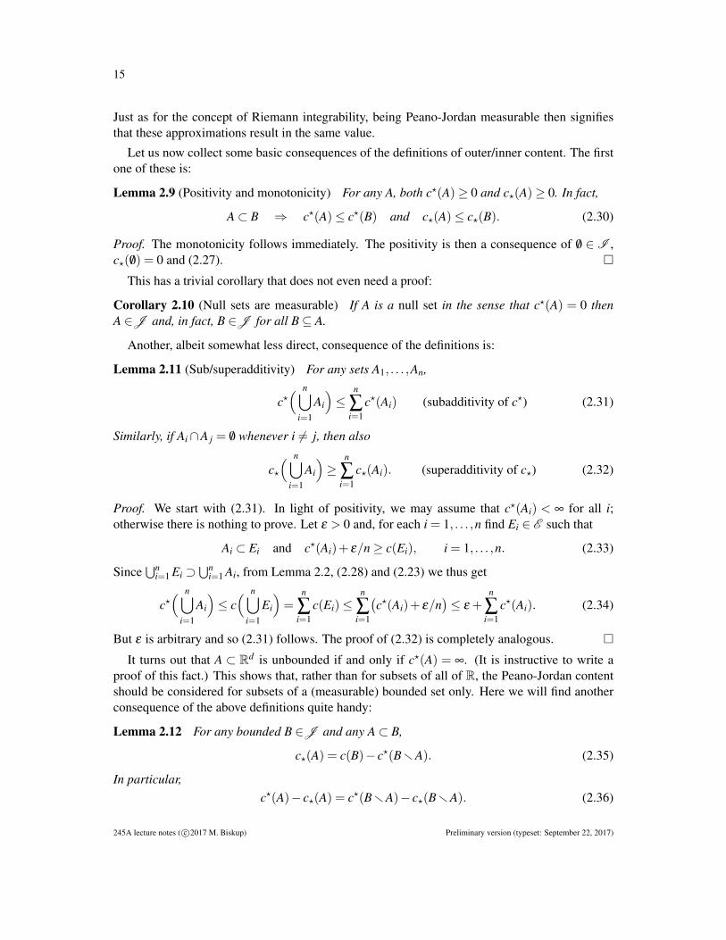
Just as for the concept of Riemann integrability, being Peano-Jordan measurable then signifiesthat these approximations result in the same value.

Let us now collect some basic consequences of the definitions of outer/inner content. The firstone of these is:

Lemma 2.9 (Positivity and monotonicity) For any A, both c?(A)≥ 0 and c?(A)≥ 0. In fact,

A⊂ B ⇒ c?(A)≤ c?(B) and c?(A)≤ c?(B). (2.30)

Proof. The monotonicity follows immediately. The positivity is then a consequence of /0 ∈ I ,c?( /0) = 0 and (2.27). �

This has a trivial corollary that does not even need a proof:

Corollary 2.10 (Null sets are measurable) If A is a null set in the sense that c?(A) = 0 thenA ∈J and, in fact, B ∈J for all B⊆ A.

Another, albeit somewhat less direct, consequence of the definitions is:

Lemma 2.11 (Sub/superadditivity) For any sets A1, . . . ,An,

c?( n⋃

i=1

Ai

)≤

n

∑i=1

c?(Ai) (subadditivity of c?) (2.31)

Similarly, if Ai∩A j = /0 whenever i 6= j, then also

c?( n⋃

i=1

Ai

)≥

n

∑i=1

c?(Ai). (superadditivity of c?) (2.32)

Proof. We start with (2.31). In light of positivity, we may assume that c?(Ai) < ∞ for all i;otherwise there is nothing to prove. Let ε > 0 and, for each i = 1, . . . ,n find Ei ∈ E such that

Ai ⊂ Ei and c?(Ai)+ ε/n≥ c(Ei), i = 1, . . . ,n. (2.33)

Since⋃n

i=1 Ei ⊃⋃n

i=1 Ai, from Lemma 2.2, (2.28) and (2.23) we thus get

c?( n⋃

i=1

Ai

)≤ c( n⋃

i=1

Ei

)=

n

∑i=1

c(Ei)≤n

∑i=1

(c?(Ai)+ ε/n

)≤ ε +

n

∑i=1

c?(Ai). (2.34)

But ε is arbitrary and so (2.31) follows. The proof of (2.32) is completely analogous. �

It turns out that A ⊂ Rd is unbounded if and only if c?(A) = ∞. (It is instructive to write aproof of this fact.) This shows that, rather than for subsets of all of R, the Peano-Jordan contentshould be considered for subsets of a (measurable) bounded set only. Here we will find anotherconsequence of the above definitions quite handy:

Lemma 2.12 For any bounded B ∈J and any A⊂ B,

c?(A) = c(B)− c?(BrA). (2.35)

In particular,c?(A)− c?(A) = c?(BrA)− c?(BrA). (2.36)


16

Proof. Fix ε > 0 and let E,F ∈ E be such that E ⊇ B (this is where we need that B is bounded)and F ⊆ A obey c(F)≥ c?(A)−ε . As E rF ∈ E by Lemma 2.2 and E rF ⊇ BrA, from (2.23)we have

c(E) = c(F)+ c(E rF)≥ c?(A)− ε + c?(BrA). (2.37)

Varying E along a sequence such that c(E) decreases to c?(B) = c(B), we get that ≤ in (2.35).For the opposite inequality, given ε > 0, we pick E,F ∈ E such that E ⊆ B and F ⊇ BrA

(again using the boundedness of B) obeys c(F) ≤ c?(BrA)+ ε . Then E rF ⊆ A and, sinceE rF ∈ E , from (2.23) we get

c(E) = c(F)+ c(E rF)≤ c?(BrA)+ ε + c?(A). (2.38)

Taking E along a sequence such that c(E) tends to c?(B) = c(B), we get ≥ in (2.35). The secondconclusion then follows by applying the first one to A and BrA. �

Note that going via complements could be considered as an alternative way to define innercontent. (We will see that this is exactly what is done for the Lebesgue measure.) With theseproperties established, we now get:

Theorem 2.13 The following holds:

(1) If A1, . . . ,An ∈J are disjoint, then also⋃n

i=1 Ai ∈J and

c( n⋃

i=1

Ai

)=

n

∑i=1

c(Ai). (2.39)

(2) If A,B are bounded and measurable, then so is A∩B and BrA.

In particular, for any bounded D ∈J , the class {A ∈J : A ⊆ D} of Peano-Jordan measurablesubsets of D is an algebra (of subsets of D) and c is an additive set function on it.

Proof. To get (1) we note that, by Lemmas 2.7 and 2.11,

n

∑i=1

c?(Ai)≤ c?( n⋃

i=1

Ai

)≤ c?

( n⋃i=1

Ai

)≤

n

∑i=1

c?(Ai). (2.40)

The left and right-hand sides agree whenever A1, . . . ,An ∈J . The claim then follows from thedefinition of measurability.

For (2) let D ∈J be bounded and note that, by Lemma 2.12, A⊆ D is measurable if and onlyif DrA is measurable. Now, for A,B⊆ D,

A∩B = Dr((DrA)∪ (DrB)

)ArB = A∩ (DrB)

(2.41)

thus show that if A,B are measurable, then so are A∩B and ArB. �

Remark 2.14 We note that all results in this section use only some very basic facts about ele-mentary sets. Namely, we need that E is closed under unions, intersections and set differencesand the content is well-defined, finite and finitely additive on E .


17

2.3 Non-measurable sets, relation to topology.

A natural question to ask is whether there are non-measurable sets — i.e., those that fail to bemeasurable. The answer to this is quite easy:

Lemma 2.15 The set A :=Q∩ [0,1] is not Peano-Jordan measurable.

Proof. The set A := Q∩ [0,1] is totally disconnected and so it contains no non-trivial intervals.Hence, we get c?(A) = 0. On the other hand, any elementary set that contains A must contain[0,1] and so c?(A)≥ c?([0,1]) = 1. �

A slightly more subtle question is what properties of sets characterize Peano-Jordan measura-bility. A simple exercise shows:

Lemma 2.16 Let A ⊂ Rd be bounded. Then A ∈J if and only if for each ε > 0 there areE,F ∈ E with F ⊆ A⊆ E and c?(E rF)< ε .

Unfortunately, this is still very much in the spirit of the original definition. A more interestingcharacterization arises when we try to relate measurability to topology. Recall that, for any setA ⊂ Rd , A denotes the closure of A while A◦ denotes the interior of A with respect to the usualEuclidean metric (and thus topology) on Rd . The boundary ∂A of A is then given by ∂A :=ArA◦.

Proposition 2.17 (Topological characterization of PJ-measuability) For any bounded A⊆ Rd ,

c?(A) = c?(A) and c?(A) = c?(A◦) (2.42)

and so A is measurable if and only if c?(A) = c?(A◦). Hence, if A is bounded and measurablethen so is any B such that A◦ ⊆ B⊆ A and c(B) = c(A) for all of these. In particular,

A ∈J ⇒ c(A) = c(A) = c(A◦). (2.43)

Finally, for A⊆ Rd bounded, Peano-Jordan measurability is characterized by

A ∈J ⇔ c?(∂A) = 0. (2.44)

Proof. We begin by proving (2.42). Let E ∈ E be an elementary sets such that A ⊆ E andc?(A)+ ε ≥ c(E). Writing E as the disjoint union

⋃ni=1 Ii of half-open boxes {Ii}, we now find

(by enlarging Ii slightly in all directions) half-open boxes I′i such that

Ii ⊆ I′i and |I′i | ≤ |Ii|+ ε/n. (2.45)

The fact that A is the smallest closed set containing A implies

A⊆n⋃

i=1

Ii ⊆n⋃

i=1

I′i = E ′ (2.46)

and we thus get

c?(A)≤n

∑i=1|I′i | ≤

n

∑i=1

(|Ii|+ ε/n

)= ε + c(E)≤ c?(A)+2ε. (2.47)

The monotonicity with respect to inclusion then yields c?(A) = c?(A). The second part of (2.42)is proved analogously: We find an elementary F ⊆ A with c?(A)− ε ≤ c(F), write it as a disjointunion of half-open boxes {Ii}, shrink these to half-open boxes I′i ⊂ (Ii)

◦ with close value of


18

content, use that A◦ is the largest open set contained in A and then apply a similar calculation asin (2.47) to conclude c?(A◦)≥ c?(A). Monotonicity then finishes the claim.

From (2.42) we then immediately get that A ∈J if and only if c?(A) = c?(A◦). Then (2.43)follows from the monotonicity of inner/outer content with respect to inclusion. Similarly we getthat, once A ∈J , A◦ ⊆ B ⊆ A implies B ∈J as well. It thus remains to prove the equivalence(2.44). Lemma 2.16 gives the implication⇒: If E,F are as in the lemma, then ∂A⊂ ErF and soc?(∂A)≤ c(E rF), which can be made as small as desired. For the opposite implication,⇐, weuse c?(∂A) = 0 to find a non-empty F ∈ E such that ∂A⊂ F◦ and c(F)< ε . Then ArF◦ ⊆ A◦.But ArF◦ is closed and so one can find E ∈ E such that

ArF◦ ⊆ E ⊆ A◦ and c?(A)− ε ≥ c(E). (2.48)

But E ∪F ∈ E and E ∪F ⊇ A. Therefore,

c?(A)≤ c(E ∪F)≤ c(E)+ c(F)< c?(A◦)+2ε. (2.49)

Hence, c?(A) = c?(A◦) and, by the first part of the claim, A ∈J . �

2.4 Connection with Riemann integral.

The fact that measurability of A implies measurability of both A and A◦ seems quite natural:indeed, we usually expect that the closure and interior of a set are more regular than the set itself.However, this conclusion has its limitations:

Lemma 2.18 There exists a closed set A⊂ [0,1] which is not Peano-Jordan measurable.

Proof (sketch). One example for this would be any fat Cantor set in [0,1]. (The existence of suchsets is what underlies Lemma 1.8.) Even more simple is an example constructed as follows: Let{qn} enumerate Q and, given ε > 0, let

A := [0,1]r⋃n≥1

(qn− ε2−n,qn + ε2−n). (2.50)

It is obvious that A is closed (possibly empty). By truncating the union at a finite n and replacingopen intervals by half-open ones, we readily find c?(A)≥ 1−2ε . On the other hand, A is totallydisconnected and so c?(A) = 0. So for ε < 1/2, A is a non-empty closed set which is not Peano-Jordan measurable. �

The conclusion that the contents of A, A and A◦ are all equal was, at the time of conceptionof this theory, considered as completely natural. However, later it was found too restrictive and,in fact, a limitation of the theory. Here we will demonstrate this further by stating without prooftwo lemmas that show that measurability is essentially equivalent to Riemann integrability.

Lemma 2.19 Let A ⊆ Rd be a bounded set. Then A ∈J if and only if 1A, the characteristicfunction of A, is Riemann integrable.

Lemma 2.20 Let a,b ∈ R obey a < b and let f : [a,b]→ [0,∞) be a function. Then

f is Riemann integrable ⇔{(x, t) ∈ [a,b]× [0,∞) : f (x)≤ t

}∈J (2.51)


19

Underlying these is the fact that the Peano-Jordan content is not countably additive. Theobstruction is explained in the next lemma, whose proof we also leave to the reader:

Lemma 2.21 There are sets A1,A2, · · · ∈J with Ai ∈ [0,1] for all i such that⋃

∞i=1 Ai 6∈J .

(Note, however, that if the union is measurable, and the sets Ai are disjoint, the content iscountably additive on this sequence.) The punchline is that, despite all of the conceptual develop-ments, we still have not left the paradigm (and thus have to face also the associated shortcomings)of Riemann integrability. However, as we will see in the next chapter, we are already on a goodway to do so.


20

3. LEBESGUE MEASURE

We can now finally start developing the theory of Lebesgue measure. There are two key im-provements compared to Peano-Jordan content: We define the outer measure using countable(as opposed to finite) covers and, abandoning the concept of inner approximations, we definemeasurability directly from outer measure.

Since we will often talk about infinite series throughout, it is useful to recall the followingbasic facts: For any sequence {ai : i ∈ N} satisfying ai ≥ 0 for each i,

∞

∑i=1

ai := limn→∞

n

∑i=1

ai (3.1)

coincides with

∑i∈N

ai := sup{

∑i∈A

ai : A⊂ N, finite}. (3.2)

In particular, the value of the infinite sum is the same for all reorderings of the sequence {ai}. Forsuch absolutely converging sums we pretty much get all of the standard properties of finite sums.For instance, if ai,bi ≥ 0 and ε ≥ 0, then

∑i∈N

(ai + εbi) = ∑i∈N

ai + ε ∑i∈N

bi. (3.3)

Similarly,0≤ ai ≤ bi ∀i ∈ N ⇒ ∑

i∈Nai ≤ ∑

i∈Nbi. (3.4)

Finally, if {ai j : i, j ∈ N} obey ai j ≥ 0, then

∑i, j∈N

ai j = ∑i∈N

∑j∈N

ai j (3.5)

(This will be later called the discrete Tonelli Theorem.) We leave (easy) verification of theseclaims to the reader.

3.1 Lebesgue outer measure.

Let us now move to the development of Lebesgue’s theory. Recall that I denotes the class ofnonempty half-open boxes in Rd and that the outer content was defined by

c?(A) := inf{ n


n⋃i=1

Ii ⊃ A}. (3.6)

The first important insight provided by Lebesgue is to enlarge the covers to countably infiniteones. This leads to:

Definition 3.1 (Lebesgue outer measure) For any A ⊂ Rd , the Lebesgue outer measure λ ?(A)of A is defined by

λ?(A) := inf

{∞


∞⋃i=1

Ii ⊃ A}, (3.7)

The outer measure has the following properties (which, as we will see, can be used to definedouter measures abstractly):


21

Proposition 3.2 (Outer measure properties) We have:

(1) (positivity) λ ?(A)≥ 0 and λ ?( /0) = 0,(2) (monotonicity) if A⊂ B, then λ ?(A)≤ λ ?(B),(3) (countable subadditivity) for any sets {Ai : i ∈ N},

λ?

(⋃i∈N

Ai

)≤ ∑

i∈Nλ?(Ai). (3.8)

Proof. (1) The real line can be covered by a countable union of unit intervals and so λ ?(A) ≥ 0for all sets A. The claim for A := /0 would be trivial if /0 were included I . However, since it isnot, for any ε > 0 we pick a collection {Ii} ⊂I such that |Ii| ≤ ε2−i. Then µ?( /0)≤∑

ni=1 |Ii| ≤ ε

and so we must have µ( /0) = 0.For (2) we just observe that if {Ii} ⊂I covers A then it covers B. So the set of covers of A is

at least as large as the set of covers of B.To get (3), we may as well assume that µ?(Ai)< ∞ for all i because otherwise the claim holds

trivially. Given ε > 0, for each i we can then find {Ii j : j ∈ N} ⊂I such that

Ai ⊂⋃j∈N

Ii j and λ?(Ai)+ ε2−i ≥ ∑

j∈N|Ii j| (3.9)

hold for each i. But then ⋃i∈N

Ai ⊂⋃

i, j∈NIi j (3.10)

and so, by the definition of λ ?,

λ?

(⋃i∈N

Ai

)≤ ∑

i, j∈N|Ii j|= ∑

i∈N∑j∈N|Ii j|

≤ ∑i∈N

(λ?(Ai)+ ε2−i)= ε + ∑

i∈Nλ?(Ai)

(3.11)

where we used (3.3–3.5) and ∑i∈N 2−i = 1 in the intermediate steps. Since this holds for all ε > 0,the claim follows. �

A natural question is whether the outer measure in fact gives a better approximation of the“volume” of A from without than the outer content does. This is settled in:

Lemma 3.3 The infimum defining λ ?(A) is unchanged if we permit Ii to be empty. In particular,for each A⊂ Rd ,

λ?(A)≤ c?(A). (3.12)

Proof. Let {Ii : i = 1, . . . ,n} be a cover of A by Ii ∈I ∪{ /0}. Given ε > 0, define I′i := Ii if Ii 6= /0and I′i :=(0,ε2−i]d otherwise. Then {I′i}⊂I is a cover of A and ∑i∈N |I′i | ≤ εd +∑i∈N |Ii|. Hence,allowing Ii to be empty does not affect the value of the infimum. The conclusion λ?(A) ≤ c?(A)then follows by comparing (3.6) with (3.7). �

The comparison with the inner content is somewhat harder. We will need a lemma:


22

Lemma 3.4 Let I ∈I and let {Ii} ⊂I be such that I ⊂⋃

i∈N Ii. Then

|I| ≤ ∑i∈N|Ii|. (3.13)

Proof. In d = 1 this may perhaps be proved by reordering the sets monotonically using transfiniteinduction but an argument based on topology is much easier. We will use that each half-openbox contains a closed box, and is contained in an open box, with both of these of nearly the samevolume. More precisely, fix ε > 0. Then there is J ∈I such that J⊂ I and |J| ≥ |I|−ε . Similarly,for each i ∈ N, there is I′i ∈I be such that Ii ⊂ (I′i )

◦ and |I′i | ≤ |Ii|+ ε2−i for each i.A key fact is that {(I′i )◦ : i ∈ N} form an open cover of the compact set J and so, by the

Heine-Borel Theorem, there is n ∈ N such that

J ⊂ J ⊂n⋃

i=1

(I′i )◦ ⊂

n⋃i=1

I′i . (3.14)

By Corollary 2.5 we thus get

|I|− ε ≤ |J| ≤n

∑i=1|I′i | ≤ ε +

n

∑i=1|Ii| ≤ ε + ∑

i∈N|Ii|. (3.15)

Since ε was arbitrary, we are done. �

This implies:

Lemma 3.5 For any A⊂ Rd ,λ?(A)≥ c?(A). (3.16)

In particular, if A ∈J , then λ ?(A) = c(A).

Proof. We start by proving the ultimate conclusion for elementary sets: If E ∈ E , then λ ?(E) =c(E). Clearly, λ ?(E)< ∞ for any E ∈ E . By Lemma 3.3, for any E ∈ E we have λ ?(E)≤ c(E).Now, given ε > 0, let {Ii} be a cover of E such that λ ?(E) ≥ ∑i∈N |Ii| − ε . Write E =

⋃nj=1 J j

with with {J j} ⊂I disjoint. Then {Ii∩ J j : i ∈ N} is a cover of J j and so, by Lemma 3.4,

|J j| ≤ ∑i∈N|Ii∩ J j|. (3.17)

On the other hand, {Ii∩ J j : j = 1, . . . ,n} is a disjoint partition of Ii and so, by Lemma 2.4,

|Ii|=n

∑j=1|Ii∩ J j|. (3.18)

Combining these we get

λ?(E)+ ε ≥ ∑

i∈N|Ii|= ∑

i∈N

n

∑j=1|Ii∩ J j|

=n

∑j=1

∑i∈N|Ii∩ J j| ≥

n

∑j=1|J j|= c(E)

(3.19)

where we again used (3.5) to write the two sums in a convenient order. Since ε was arbitrary, weget λ ?(E) = c(E) as claimed.


23

Now recall that c?(A) is the supremum of c(E) over all E ∈ E with E ⊂ A. Thus we get

c?(A) = sup{

λ?(E) : E ∈ E , E ⊂ A

}. (3.20)

But Proposition 3.2(2) gives λ ?(E) ≤ λ ?(A) for all such E and so c?(A) ≤ λ ?(A) as well. IfA ∈J , then c?(A) = c?(A) and so they also equal λ ?(A). �

The above argument has a simple, albeit quite non-trivial, consequence:

Corollary 3.6 If {Ii} ⊂I are disjoint, then

λ?

(⋃i∈N

Ii

)= ∑

i∈N|Ii| (3.21)

In particular, for any pair of disjoint collections {Ii} ⊂I and {J j} ⊂I ,⋃i∈N

Ii =⋃j∈N

J j ⇒ ∑i∈N|Ii|= ∑

j∈N|J j| (3.22)

Proof. By subadditivity (Proposition 3.2(3)) we have “≤.” For the other direction we use that⋃i∈N Ii ⊃ E for E :=

⋃ni=1 Ii. This is an elementary set so the previous lemma gives us

λ?

(⋃i∈N

Ii

)≥ λ

?

( n⋃i=1

Ii

)= c( n⋃

i=1

Ii

)=

n

∑i=1|Ii| (3.23)

by Proposition 3.2(2) and Theorem 2.13(1). Taking n→ ∞, we get “≥” as well. The second partfollows trivially from the first. �

We remark that, although (3.22) is quite intuitive, a direct proof may be quite challenging.

Lemmas 3.3 and 3.5 can be further strengthened for bounded sets. Given a bounded A ⊂ Rd

and any I ∈I such that A⊂ I, define

λ?(A) := |I|−λ?(I rA) (3.24)

This is the inner Lebesgue measure. As is easy to check (using, e.g., Corollary 3.6), this definitionis independent of the choice of I. We then have:

Lemma 3.7 Let A⊂ Rd be bounded. Then

c?(A)≤ λ?(A)≤ λ?(A)≤ c?(A). (3.25)

In particular, if A ∈J , then λ ?(A) = λ?(A).

Proof. This is a direct consequence of Lemmas 3.3, 3.5 and 2.12. �

This property suggest calling a bounded set A ⊂ Rd to be Lebesgue measurable wheneverλ ?(A) = λ?(A). The conclusion of the lemma is then that every Peano-Jordan measurable setis automatically Lebesgue measurable. Unfortunately, defining Lebesgue measurability via thisroute would make the whole concept restricted to bounded sets. So another, more general, defini-tion will need to be employed that subsumes the inner/outer measure definition for bounded sets.


24

3.2 Lebesgue measurable sets.

Our definition of measurability will be tied to topology. Recall that a set O⊂ Rd is open if, witheach point x, it contains a ball of a positive radius centered at x. The class of open sets defines atopology. The following property ties topology to the Lebesgue outer measure:

Lemma 3.8 For each A⊂ Rd ,

λ?(A) = inf

{λ?(O) : O⊂ A, open

}. (3.26)

Proof. Whenever A⊂O, we have λ ?(A)≤ λ ?(O) by Proposition 3.2(2). Hence, λ ?(A) is at mostthe infimum. For the opposite inequality assume, without loss of generality, that λ ?(A) < ∞.Then for each ε > 0 there are {Ii} ⊂ I such that A ⊂

⋃i∈N Ii and λ ?(A)+ ε ≥ ∑i∈N |Ii|. Now

enlarge each Ii to get I′i open with I′i ⊃ Ii and |I′i | ≤ |Ii|+ ε2−i. Define O :=⋃

i∈N I′i . Then O isopen and O⊃ A. Moreover,

λ?(O)≤ ∑

i∈N|I′i | ≤ ε + ∑

i∈N|Ii| ≤ 2ε +λ

?(A). (3.27)

Since ε was arbitrary, the claim follows. �

When an open set O⊃ A is gradually decreased along a sequence On so that λ ?(On) ↓ λ ?(A),we may ask whether λ ?(On rA) tends to zero as well. We may even consider the intersectionB :=

⋂n∈N On and ask about the value of λ ?(BrA). None of these seem to hold generally and so

we single out a class of sets for which these properties can be proved:

Definition 3.9 (Lebesgue measurable sets) A set A ⊂ Rd is Lebesgue measurable if for ev-ery ε > 0 there is an open set O⊂ A such that λ ?(OrA)< ε .

We will write L or, when explicit mention of dimension is necessary, L (Rd) to denote theclass of Lebesgue measurable sets in Rd . This class has the following properties:

Proposition 3.10 We have:(1) if O⊂ Rd is open, then O ∈L (Rd),(2) if {An} ⊂L (Rd), then also

⋃n∈N An ∈L (Rd),

(3) if C ⊂ Rd is closed, then C ∈L (Rd),(4) if λ ?(A) = 0 then A ∈L (Rd),(5) if A ∈L (Rd) then also Ac ∈L (Rd).

Proof of (1) and (2). (1) is trivial as for A open one takes O := A. For (2), let {An} ⊂L (Rd).Then, given ε > 0, we can find open sets On ⊃ An such that λ ?(On rAn) < ε2−n. Then A :=⋃

n∈N An ⊂ O :=⋃

n∈N On with O open and, since⋃n∈N

On r⋃

n∈NAn ⊂

⋃n∈N

(On rAn), (3.28)

the monotonicity and countable subadditivity of λ ? show

λ?(An rOn)≤ ∑

n∈Nλ?(On rAn)≤ ∑

n∈Nε2−n = ε. (3.29)

Hence A ∈L (Rd) as well. �


25

For the proof of the remaining parts, we need some lemmas:

Lemma 3.11 If O⊂ Rd is open then there are {Ii} ⊂I disjoint such that O =⋃

i∈N Ii.

Proof. This is based on the use of dyadic partitions of Rn. Let

Dn :={(

k12−n,(k1 +1)2−n]×·· ·× (kd2−n,(kd +1)2−n] : k1, . . . ,kd ∈ Z}. (3.30)

We call elements of Dn the dyadic (half-open) cubes of base 2−n. These are rather special because,for any m,n ∈ N with m≤ n we have

I ∈Dm, J ∈Dn ⇒ J ⊆ I OR I∩ J = /0. (3.31)

This is because the partitions induced by Dn and Dm are nested.Now pick O open and define a sequence of sets An inductively as follows: Set A1 := O and,

given An, let An+1 be the set of all x ∈ An such that if I ∈ Dn+1 obeys x ∈ I, then An r I 6= /0. (Inother words, An+1 is An with all I ∈Dn+1 that fit entirely into An removed.) Then

An rAn−1 =

m(n)⋃i=1

Jn,i (3.32)

for some Jn,i ∈Dn with {Jn,i : n∈N, i= 1, . . . ,m(n)} disjoint. Obviously, An decreases with n; weclaim that An ↓ /0. Indeed, with each x ∈O, the set O contains an open Euclidean ball containing xand thus also a dyadic cube I ∈Dn+1 with x ∈ I, for some n ∈ N. By (3.31), either this I is eitherentirely contained in one of dyadic cubes constituting OrAn, or is disjoint from all of them. Inthe former case x ∈ OrAn, in the latter case x ∈ ArAn+1. Hence,

O = A1 =⋃n≥2

(An rAn−1) =⋃n≥2

m(n)⋃i=1

Jn,i. (3.33)

Since the dyadic cubes on the right are by construction disjoint, the claim follows. �

The other lemma gives a statement concerning additivity of the outer measure λ ?. We notethat outer measures are generally not additive — i.e., we may have λ ?(A∪B) < λ ?(A)+λ ?(B)even if A,B⊂Rd obey A∩B = /0. However, if we assume that A and B are separated by a positivedistance, then additivity holds:

Lemma 3.12 Let ρ(A,B) := inf{|x− y|∞ : x ∈ A, y ∈ B} where |x− y|∞ := maxi=1,...,d |xi− yi|.Then for all A,B⊂ Rd ,

ρ(A,B)> 0 ⇒ λ?(A∪B) = λ

?(A)+λ?(B). (3.34)

Proof. In light of subadditivity of λ ?, we only need to show “≥” which in turn permits us toassume λ ?(A∪B)< ∞. We will use the fact that, by Lemma 2.4, given any δ > 0, if every cover{Ii} of a set by half-open boxes can be refined into a cover by boxes whose every side is lessthan δ without changing ∑i∈N |Ii|.

Thus, pick δ := 13 ρ(A,B) and let {Ii} be a cover of A∪B by half-open boxes (or empty sets)

with the largest side at most δ so that

λ?(A∪B)+ ε ≥ ∑

i∈N|Ii|. (3.35)


26

Define S := {i ∈ N : Ii∩A 6= /0} and note that then A⊂⋃

i∈S Ii. By our choice of δ , i ∈ S impliesIi∩B = /0 and so also B⊂

⋃i∈NrS Ii. Hence, by the definition of λ ? and (3.35),

λ?(A)+λ

?(B)≤∑i∈S|Ii|+ ∑

i∈NrS|Ii|= ∑

i∈N|Ii| ≤ λ

?(A∪B)+ ε. (3.36)

Since ε was arbitrary, the claim thus follows. �

We may now finish the proof of Proposition 3.10:Proof of (3). Pick C ⊂ Rd closed and assume, for the start, that C is also bounded (and thuscompact). If O is an open set such that O⊃C, then also OrC is open. By Lemma 3.11 there aredisjoint {Ii} ⊂I so that

OrC =⋃i∈N

Ii. (3.37)

By Corollary 3.6,λ?(OrC) = ∑

i∈N|Ii|. (3.38)

Next let ε > 0 and let I′i ∈I be such that I′i ⊂ Ii and |I′i |+ε2−i ≤ |Ii|. By the Bolzano-Weierstrasstheorem, two compact sets A,B ⊂ Rd with A∩B = /0 necessarily obey ρ(A,B) > 0, and since afinite union of compact sets is compact,

ρ

(C,

n⋃i=1

I′i)> 0, n ∈ N. (3.39)

Corollary 3.6 gives λ ?(⋃n

i=1 I′i ) = ∑ni=1 |I′i | and, by (3.37), the monotonicity of λ ?, Lemma 3.12

and the construction of {I′i} we thus get

λ?(O)≥ λ

?(

C∪n⋃

i=1

I′i)

= λ?(C)+λ

?( n⋃

i=1

I′i)= λ

?(C)+n

∑i=1|I′i |

≥ λ?(C)− ε +

n

∑i=1|Ii|.

(3.40)

With the help of (3.38), the limits n→ ∞ and ε ↓ 0 yield

λ?(OrC) = ∑

i∈N|Ii| ≤ λ

?(O)−λ?(C). (3.41)

Since C is bounded, λ ?(C) < ∞. By Lemma 3.8 for each ε > 0 there is O ⊃ C open so thatλ ?(O) ≤ λ ?(C)+ ε . The above then shows λ ?(OrC) < ε and so C ∈L (Rd). This proves (3)for every C compact. As every closed set in Rd can be written as a countable union of compactsets, (2) extends this to general closed sets as well. �

Proof of (4). Let A⊂Rd be such that λ ?(A) = 0. Since Rd is open, the infimum in Lemma 3.8 isnot over an empty set. Hence, for each ε > 0 there is an O ⊃ A open such that λ ?(O) < ε . Butλ ?(OrA)≤ λ ?(O) and so A ∈L (Rd) as claimed. �


27

Proof of (5). Let A ∈ L (Rd). Then there are On ⊃ A open with λ ?(On r A) → 0. DefineB :=

⋃n∈N Oc

n and note that AcrB⊂AcrOcn for each n∈N. But A⊂On implies AcrOc

n =OnrAand so

λ?(Ac rB)≤ λ

?(Ac rOcn) = λ

?(On rA) −→n→∞

0. (3.42)

Hence λ ?(Ac rB) = 0 and, by (4), Ac rB ∈ L (Rd). But B ∈ L (Rd) as well by (1,2,3) and,since B⊂ Ac, also Ac = B∪Ac ∈L (Rd) by (2). �

Since /0 and Rd are automatically open, Proposition 3.10 shows that the structure of L (Rd)fits into the following important concept:

Definition 3.13 A class M of subsets of a set X is a σ -algebra if

(1) /0,X ∈M ,(2) A ∈M ⇒ Ac ∈M ,(3) {An} ∈M ⇒

⋃n∈N An ∈M .

Note that this specializes the concept of an algebra, introduce earlier in these notes, by requir-ing that also countable unions of sets in M are contained in M . Obviously, M is then closedalso under countable intersection and set differences.

An important question is whether the characterization we used to define L (Rd) is unique.Consider the following classes of sets:

Fσ (Rd) :={⋃

n∈NKn : Kn ⊂ Rd , closed

}(3.43)

and

Gδ (Rd) :={⋂

n∈NOn : On ⊂ Rd , open

}(3.44)

As a simple consequence of Proposition 3.10, we get:

Corollary 3.14 (Alternative definitions of Lebesgue measurable sets) A ∈L (Rd) is equivalentto any of these three statements:

(1) For each ε > 0 there is K ⊂ A closed so that λ ?(ArK)< ε .(2) There is B ∈ Gδ (Rd) such that B⊃ A and λ ?(BrA) = 0.(3) There is C ∈Fσ (Rd) such that C ⊂ A and λ ?(ArC) = 0.

Proof. (1) If O⊃ Ac is open then K := Oc is closed with K ⊂ A and ArK = OrAc. For (2) usethe argument from the proof (5) of Proposition 3.10; (3) then follows by complementation. �

3.3 Lebesgue measure.

We now move on to defining the Lebesgue measure. Here is a general definition:

Definition 3.15 (General measure) Let M be a σ -algebra of subsets of a set X . The mapµ : M → [0,∞] is a measure if

(1) µ( /0) = 0, and


28

(2) if {An} ⊂M are disjoint, then

µ

(⋃n∈N

An

)= ∑

n∈Nµ(An). (3.45)

Condition (2) is referred to as countable subadditivity of µ .

The main purpose of condition (1) is to ensure that µ is not identically infinity on M . (Notethat, by (2), µ( /0) can only take values 0 or ∞.) Going back to our main line of reasoning, we nowclaim:

Proposition 3.16 The restriction of λ ? to L (Rd) is a measure.

Proof. We have λ ?( /0) = 0 so we only need to show that λ ? acts additively on countable unionsof disjoint sets from L (Rd). First we prove finite additivity for bounded sets. Let A,B ∈L (Rd)be bounded. By Corollary 3.14, for each ε > 0 there are closed sets K1 ⊂ A and K2 ⊂ B (thuscompact) such that λ ?(ArK1),λ

?(BrK2) < ε . If also A∩B = /0, the fact that K1 and K2 arecompact ensures that ρ(K1,K2)> 0. Hence

λ?(K1∪K2) = λ

?(K1)+λ?(K2) (3.46)

by Lemma 3.12. But λ ?(A)≤ λ ?(K1)+ε and λ ?(B)≤ λ ?(K2)+ε by subadditivity of λ ? and so

λ?(A∪B)≥ λ

?(K1∪K2)≥ λ?(A)+λ

?(B)−2ε. (3.47)

By subadditivity again, λ ? is additive on finite unions of bounded disjoint sets.Now consider a countable collection {An} ⊂L (Rd) of bounded disjoint sets. Then

λ?(⋃

n∈NAn

)≥ λ

?( n⋃

i=1

Ai

)=

n

∑i=1

λ?(Ai)

n→∞∑n∈N

λ?(An) (3.48)

where we used finite additivity to get the middle equality. Hence, λ ? is additive on countableunions of disjoint bounded sets. To remove the boundedness restriction, let D be a partitionof Rd into shifts of (0,1]d by integers in each lattice direction. If {Dm} enumerates D and{An} ⊂L (Rd) is a disjoint collection, then

λ?(⋃

n∈NAn

)= λ

?( ⋃

m,n∈N(An∩Dm)

)= ∑

m,n∈Nλ?(An∩Dm) = ∑

n∈N∑

m∈Nλ?(An∩Dm)

= ∑n∈N

λ?(⋃

n∈N(An∩Dm)

)= ∑

n∈Nλ?(An)

(3.49)

where the second and fourth equality follow because {(An ∩Bm) : m,n ∈ N} is a countable col-lection of disjoint bounded sets, the third equality is a consequence of (3.5) and the last equalityfollows because {Dm : m ∈ N} form a partition of Rd . �

Definition 3.17 (Lebesgue measure) Let us write λ (A) for λ ?(A) whenever A ∈L (Rd). Wewill call λ (A) the Lebesgue measure of A.

Returning to the concept of inner measure for bounded sets, we now observe:


29

Proposition 3.18 Let A⊂ Rd be bounded. Then A ∈L (Rd) if and only if λ ?(A) = λ?(A).

Proof. Homework exercise. �

The Lebesgue measure has a lot of symmetries. In particular, we have:

Proposition 3.19 (Translation invariance) For any A⊂ Rd and z ∈ Rd , define

z+A := {z+ x : x ∈ A} (3.50)

Then for all A ∈L (Rd) and all z ∈ Rd ,

z+A ∈L (Rd) and λ (z+A) = λ (A). (3.51)

Proof. Homework exercise (easy). �

The Lebesgue measure is further invariant under rotations (i.e., linear maps induced by orthog-onal matrices) and transforms nicely under dilations. We will revisit this question later.

3.4 Convergence Theorems.

As a corollary to the definition of measure, we get useful convergence theorems. (We state thesefor a general measure as no other properties are needed.) The first theorem deals with mono-tone sequences. Recall that we write An ↑ A whenever n 7→ An is increasing and A =

⋃n∈N An.

Similarly, we write An ↓ A whenever n 7→ An is decreasing and A =⋂

n∈N An.

Theorem 3.20 (Monotone Convergence Theorem for sets) Let µ be a measure on σ -algebra M .Let {An} ∈M . Then we have:

(1) If An ↑ A, then µ(An) ↑ µ(A).(2) If An ↓ A and µ(A1)< ∞, then µ(An) ↓ µ(A).

Proof. If An ↑ A then {An rAn−1 : n ∈ N}, where A0 := /0, are disjoint with

An =n⋃

k=1

(Ak rAk−1) and A =⋃k∈N

(Ak rAk−1). (3.52)

Therefore,

µ(An) =n

∑k=1

µ(Ak rAk−1) −→n→∞

∑k∈N

µ(Ak rAk−1) = µ(A). (3.53)

This proves (1).For (2), let An ↓ A. Then A1 rAn ↑ A1 rA and so, by µ(A1)< ∞,

µ(An) = µ(A1)−µ(A1 rAn) −→n→∞

µ(A1)−µ(A1 rA) = µ(A). (3.54)

where the limit follows by part (1). �

Our next convergence result addresses the situation when the sequence of sets is not necessarilymonotone. Given a collection of sets {An}, we define

limsupn→∞

An :=⋂n≥1

⋃k≥n

Ak (3.55)


30

andliminf

n→∞An :=

⋃n≥1

⋂k≥n

Ak (3.56)

Obviously, liminfn→∞ An ⊂ limsupn→∞ An and so we say

limn→∞

An exists if limsupn→∞

An = liminfn→∞

An (3.57)

The limit is the the common value of the limes inferior and the limes superior. As is easy tocheck, this subsumes the aforementioned case when {An} is either increasing or decreasing.

Lemma 3.21 (Fatou’s lemma for sets) Let µ be a measure on a σ -algebra M . Let {An} ⊂M .Then liminfn→∞ An ⊂M and

µ(liminf

n→∞An)≤ liminf

n→∞µ(An). (3.58)

Proof. For each m≥ n we have Am ⊃⋂

k≥n Ak. Hence,

infm≥n

µ(Am)≥ µ

(⋂k≥n

Ak

). (3.59)

Since⋂

k≥n Ak ↑ liminfn→∞ An, the claim follows from the Upward Monotone Convergence The-orem for sets. �

Due to the asymmetry between the Upward and Downward version of the Monotone Conver-gence Theorem for sets, the corresponding theorem for limes superior requires bounded mea-sures:

Lemma 3.22 (Reverse Fatou’s lemma for sets) Let µ be a measure on a σ -algebra M . Let{An} ⊂M . Then limsupn→∞ An ⊂M and, if there is B ∈M with µ(B) < ∞ and B ⊃ An foreach n, then

µ(limsup

n→∞

An)≤ limsup

n→∞

µ(An). (3.60)

Proof. We havelimsup

n→∞

An = Br liminfn→∞

(BrAn) (3.61)

Once µ(B)< ∞, the result follows by complementation from Fatou’s lemma. �

When the limit of An exists, these simplify into:

Theorem 3.23 (Dominated Convergence Theorem for sets) Let µ be a measure on σ -algebra M .Let {An} ⊂M be such that limn→∞ An exists. Then limn→∞ An ∈M and if there is a B ∈M withµ(B)< ∞ and B⊃ An for all n, we have

µ(

limn→∞

An)= lim

n→∞µ(An). (3.62)

(In particular, the limit on the right exists, albeit only in [0,∞].)

Proof. Apply Fatou and reverse Fatou to get

limsupn→∞

µ(An)≤ µ(

infn→∞

An)≤ liminf

n→∞µ(An). (3.63)

Hence the limit of µ(An) exists and equals the measure of the limit of An. �


31

We remark that, perhaps with the exception of the Monotone Convergence Theorem, the aboveresults are far more frequently used in their versions for integrals of measurable functions.

3.5 Nonmeasurable sets.

We have seen that all open and closed sets are Lebesgue measurable, and so are the sets inFσ (Rd) and Gδ (Rd) — and in particular, also the counterexample to Peano-Jordan measurabilityfrom the proof of Lemma 2.18. In fact, for any set A ⊂L (Rd), if we denote by

Aσ :={⋃

n∈NAn : An ∈A

}(3.64)

and

Aδ :={⋂

n∈NOn : An ∈A

}(3.65)

the sets in Aδ ,Aσ ,Aδσ := (Aδ )σ , Aσδ := (Aσ )δ ), Aσδσ := (Aσδ )σ , etc., all lie in L (Rd). Aquestion thus arises whether there are in fact any sets that are not Lebesgue measurable. This wasresolved rather soon after Lebesgue set up his theory:

Theorem 3.24 (Vitali) Assuming the Axiom of Choice, there is A⊂ [0,1] such that A 6∈L (Rd).

Here we recall:

Axiom of Choice For any set X there is a map f : 2X → X so that f (A) ∈ A for every A ∈ 2X .

In words, the Axiom of Choice guarantees that from each subset A of X we can choose arepresentative element f (x) that, naturally, belongs to A. This axiom of set theory (not the partof the standard ZF system) is often invoked in analysis where a proof without it is not known (orknown not to be possible, as is the example of Vitali’s theorem).Proof of Theorem 3.24. Define an equivalence relation ∼ on R by saying x ∼ y if and onlyif x− y ∈ Q. Denoting by [x] := {y ∈ R : y ∼ x} the equivalence class containing x, we haveR =

⋃x∈R[x]. The Axiom of Choice guarantees the existence of a map f : {[x] : x ∈ R} → R so

that f ([x])∈ [x]. By taking this map modulo integers, we may (and will) assume that f ([x])∈ [0,1)for all x ∈ R.

Let A := { f (x) : x ∈ R}. Then A⊂ [0,1]. Writing q+A := {q+ x : x ∈ A}, we now claim

∀q,q′ ∈Q : q+A∩q′+A 6= /0 ⇔ q = q′ (3.66)

Indeed, if x,y ∈ A are such that x+q = y+q′ for q,q′ ∈ Q, then y ∈ [x]. But A contains at mostone representative of [x] and so y = x. Then also q = q′. (The other direction is trivial.)

From the above we know that {q+A : q ∈Q} are disjoint. Next we observe⋃q∈Q

(q+A) = R. (3.67)

This is because each y ∈ R belongs to [x] for some x ∈ A. Finally, we note that, since A⊂ [0,1],⋃q∈[0,1]∩Q

(q+A)⊂ [0,2]. (3.68)


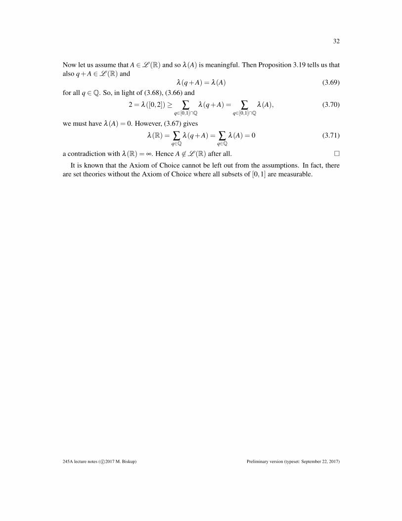
32

Now let us assume that A ∈L (R) and so λ (A) is meaningful. Then Proposition 3.19 tells us thatalso q+A ∈L (R) and

λ (q+A) = λ (A) (3.69)for all q ∈Q. So, in light of (3.68), (3.66) and

2 = λ ([0,2])≥ ∑q∈[0,1]∩Q

λ (q+A) = ∑q∈[0,1]∩Q

λ (A), (3.70)

we must have λ (A) = 0. However, (3.67) gives

λ (R) = ∑q∈Q

λ (q+A) = ∑q∈Q

λ (A) = 0 (3.71)

a contradiction with λ (R) = ∞. Hence A 6∈L (R) after all. �

It is known that the Axiom of Choice cannot be left out from the assumptions. In fact, thereare set theories without the Axiom of Choice where all subsets of [0,1] are measurable.


33

4. LEBESGUE INTEGRAL: BOUNDED CASE

Having developed the concept of the Lebesgue measure, we will now move to defining theLebesgue integral. It would be a waste to restrict attention to integrals with respect to theLebesgue measure only; indeed, working with general measure adds only little extra work. (Wewill still call the integral the Lebesgue integral, though.) The theory is best appreciated if startedfrom integrating bounded functions on sets of finite measure.

4.1 Bounded functions on finite measure spaces.

Recall the definitions of the σ -algebra and general measure from Definitions 3.13 and 3.15. Westart with some standard notions:

Definition 4.1 A pair (X ,F ), where F is a σ -algebra of subsets of X , is called a measurablespace. If µ is a measure on (X ,F ), we call (X ,F ,µ) a measure space. The measure space(X ,F ,µ) is finite if µ(X)< ∞. It is a probability space if µ(X) = 1.

Let (X ,F ) be a measurable space and consider a bounded function f : X → R. The definitionof the Lebesgue integral we will give is similar to Darboux’ version of Riemann’s integral: Wewill approximate f from below and above by “piece-wise” constant functions — to be calledsimple functions — for which the integral is canonically defined. If the resulting upper and lower(Lebesgue) integrals coincide, we proclaim the common value the (Lebesgue) integral of f . Thesimple functions are defined as follows:

Definition 4.2 Let (X ,F ) be a measurable space. A map φ : X → R is a simple function ifthere are disjoint sets {A1, . . . ,An} ⊂F and values a1, . . . ,an ∈ R such that

φ =n

∑i=1

ai1Ai . (4.1)

Obviously, we may even require that the values {ai} are distinct and non-zero. Under thisrestriction, the representation (4.1) of φ is unique. The integral of simple functions with respectto a measure µ on (X ,F ) is then defined canonically by∫

φ dµ :=n

∑i=1

ai µ(Ai). (4.2)

Here we see the reason for requiring the Ai’s to be measurable.The distinctness restriction on {ai} are sometimes inconvenient to impose. However, without

this restriction the representation of the simple function is no longer unique and one then needsto check that the integral does not depend on the representation. It suffices to prove:

Lemma 4.3 (Independence of representation) Suppose µ(X) < ∞ and consider a collection ofnumbers a1, . . . ,an,b1, . . . ,bm ∈ R and setsA1, . . . ,An,B1, . . . ,Bm ∈ F be such that both fami-lies {Ai} and {B j} are disjoint and {b j} are distinct. If

n

∑i=1

ai1Ai(x) =m

∑j=1

b j1B j(x), x ∈ X , (4.3)


34

then alson

∑i=1

ai µ(Ai) =m

∑j=1

b j µ(B j). (4.4)

In particular, (4.2) applies whenever (4.1) holds, regardless of distinctness restriction on {ai}.

Proof. A term with ai = 0 or b j = 0 can be left out of the expression so let us also assume thata1, . . . ,an,b1, . . . ,bm 6= 0. Then (4.3) shows

⋃ni=1 Ai =

⋃mj=1 B j. Hence {Ai} and {B j} are both

disjoint partitions of this union and so

Ai =m⋃

j=1

(Ai∩B j) and B j =n⋃

i=1

(Ai∩B j). (4.5)

Since alsoAi∩B j 6= /0 ⇒ ai = b j (4.6)

we thus haven

∑i=1

ai µ(Ai) =n

∑i=1

m

∑j=1

ai µ(Ai∩B j)

=m

∑j=1

n

∑i=1

b j µ(Ai∩B j),=m

∑j=1

b j µ(B j)

(4.7)

where we also used finite additivity of µ . �

The integral in (4.2) has the following immediate properties:

Lemma 4.4 Suppose µ(X)< ∞. Then we have:(1) If φ1, φ2 are simple then so is φ1 +φ2 and∫

(φ1 +φ2)dµ =∫

φ1 dµ +∫

φ2 dµ. (4.8)

(2) If φ is simple and c ∈ R, then cφ is simple and∫(cφ)dµ = c

∫φ dµ. (4.9)

(3) If φ1, φ2 are simple with φ1 ≤ φ2, then∫φ1 dµ ≤

∫φ2 dµ. (4.10)

(4) If φ is simple, then ∣∣∣∫ φ dµ

∣∣∣≤ (supx∈X|φ(x)|

)µ(X). (4.11)

Proof. Property (2) is immediate from the definition of the integral. An important technical pointfor the proof of (1) and (3) is that if φ1 and φ2 are simple functions then there are disjoint sets{Ai} and (not necessarily distinct) collections of numbers a1, . . . ,an and b1, . . . ,bn such that

φ1 =n

∑i=1

ai 1Ai and φ2 =n

∑i=1

bi 1Ai . (4.12)


35

Using this representation of both simple functions, to get (1) it then suffices to note that φ1+φ2 =

∑ni=1(ai +bi)1Ai and so∫

(φ1 +φ2)dµ =n

∑i=1

(ai +bi)µ(Ai)

=n

∑i=1

ai µ(Ai)+n

∑i=1

bi µ(Ai) =∫

φ1 dµ +∫

φ2 dµ,

(4.13)

where in the first and third inequality we used Lemma 4.3.For (3) we in turn note that, for the representation as in (4.12), φ1≤ φ2 implies ai≤ bi whenever

Ai 6= /0 and so (again with the help of Lemma 4.3),∫φ1 dµ =

n

∑i=1

ai µ(Ai)≤n

∑i=1

bi µ(Ai) =∫

φ2 dµ. (4.14)

Finally, for property (4) we use the fact that φ1 :=(supx∈X |φ(x)|

)is simple and −φ1 ≤ φ ≤ φ1.

So, by (2) and (3) we have

−(supx∈X|φ(x)|

)µ(X) =

∫(−φ1)dµ ≤

∫φ dµ ≤

∫φ1 dµ =

(supx∈X|φ(x)|

)µ(X). (4.15)

The claim in (4) now follows. �

Now let us assume that f : X → R is a bounded function and that µ(X) < ∞. Similarly tothe Darboux approach to Riemann integration, we define the lower Lebesgue integral of f withrespect to µ by ∫

f dµ := sup{∫

φ dµ : φ simple, φ ≤ f}

(4.16)

and the upper Lebesgue integral of f with respect to µ by∫f dµ := inf

{∫φ dµ : φ simple, φ ≥ f

}. (4.17)

By Lemma 4.4 φ1 ≤ f ≤ φ2 implies∫

φ1 dµ ≤∫

φ2 dµ and so∫f dµ ≤

∫f dµ. (4.18)

Lemma 4.4(4) also shows that both integrals are finite. We then define:

Definition 4.5 (Lebesgue integrability) Assuming µ(X)< ∞, a bounded function f : X → R issaid to be Lebesgue integrable with respect to µ , or just integrable, if∫

f dµ =∫

f dµ. (4.19)

For integrable f we then define its Lebesgue integral with respect to µ by∫f dµ :=

∫f dµ

(=∫

f dµ

). (4.20)

The integral thus defined naturally extends, and inherits many properties we already showedfor, the integral of simple functions:


36

Lemma 4.6 Suppose µ(X)< ∞ and let f ,g : X → R below be bounded functions. Then:(0) If f is simple then f is integrable and its Lebesgue integral coincides with that in (4.2).(1) If f ,g are integrable then so is f +g and∫

( f +g)dµ =∫

f dµ +∫

gdµ. (4.21)

(2) If f is integrable and c ∈ R, then c f is simple and∫(c f )dµ = c

∫f dµ. (4.22)

(3) If f , g are integrable with f ≤ g, then∫f dµ ≤

∫gdµ. (4.23)

(4) If f is integrable, then ∣∣∣∫ f dµ

∣∣∣≤ (supx∈X| f (x)|

)µ(X). (4.24)

Proof. (0) If f is simple and φ ≤ f ≤ φ ′, then∫

φdµ ≤∫

f dµ ≤∫

φ ′dµ . This shows that the upperintegral of f is at least

∫f dµ while the lower integral is at most

∫f dµ . But f is an upper/lower

bound on itself, so the two integrals actually coincide and equal∫

f dµ as claimed.(1) If φ1,φ2 are simple functions such that φ1 ≤ f φ2 and φ ′1,φ

′2 are simple functions such that

φ ′1 ≤ g≤ φ ′2, then φ1 +φ2 ≤ f +g≤ φ ′1 +φ ′2. Hence we get∫f dµ +

∫gdµ ≤

∫( f +g)dµ ≤

∫( f +g)dµ ≤

∫f dµ +

∫gdµ, (4.25)

where all integrals are finite. So if both f and g are integrable, the extreme left and right handsides coincide and the claim follows.

(2) If c≥ 0 and φ1 ≤ f ≤ φ2 then cφ1 ≤ c f ≤ cφ2. This shows

c∫

f dµ ≤∫(c f )dµ ≤

∫(c f )dµ ≤ c

∫f dµ. (4.26)

If f is integrable, we right and left hand sides are equal. For c < 0 the proof is completelyanalogous except that φ1 ≤ f ≤ φ2 now implies cφ2 ≤ c f ≤ cφ1. The same argument follows withthe roles of upper/lower integrals interchanged in appropriate places.

(3) Let f ≤ g. If φ is simple with φ ≤ f then also φ ≤ g. It follows that∫f dµ ≤

∫gdµ. (4.27)

For integrable f and g, this induces a similar comparison of the Lebesgue integrals.(4) If φ := supx∈X | f (x)|, then φ is simple with −φ ≤ f ≤ φ . It follows that

−(supx∈X| f (x)|

)µ(X) =

∫(−φ)dµ ≤

∫f dµ ≤

∫f dµ ≤

∫φ dµ =

(supx∈X| f (x)|

)µ(X). (4.28)

For f integrable, this wraps up into the claimed inequality. �

The properties in the above lemma can be summarized by saying that the map f 7→∫

f dµ is apositive bounded linear functional on the linear space of bounded integrable functions.


37

In integration theory one sometimes wants to integrate f only on a subset of the underlyingspace. For this we note:

Lemma 4.7 Let µ(X) < ∞ and let f : X → R be a bounded integrable function. Then f1A isintegrable for all A ∈F as well.

Proof. Let A ∈F . Since f is integrable, for each ε > 0 there are simple functions φ ,φ ′ suchthat φ ≤ f ≤ φ ′ and

∫φ ′dµ−

∫φ dµ < ε . But then both φ1A and φ ′1A are simple functions with

φ1A ≤ f1A ≤ φ ′1A and∫(φ ′1A)dµ−

∫(φ1A)dµ =

∫((φ ′−φ)1A)dµ ≤

∫(φ ′−φ)dµ < ε. (4.29)

So f1A is integrable as well. �

In light of this observation, we put forward:

Definition 4.8 Given any A ∈F , we will say that f : X → R is integrable on A whenever f1Ais integrable. In this case we write ∫

Af dµ :=

∫( f1A)dµ. (4.30)

It is a straightforward exercise, albeit somewhat lengthy, to prove:

Lemma 4.9 Let (X ,F ,µ) be a measure space and let A ∈F . Define

FA := {B∩A : B ∈F} and µA(B) := µ(A∩B). (4.31)

Then (X ,FA,µA) is a measure space. Moreover, if µ(X) < ∞ and f : X → R is bounded andintegrable on A (with respect to µ), then the restriction fA of f to A is integrable with respectto µA and ∫

Af dµ =

∫fA dµA. (4.32)

We leave the proof of this lemma to the reader.

4.2 Integrability vs measurability.

We note that, in all of the above statements, it would suffice to have µ only finitely additive on Fwith µ(X) < ∞. (Reformulating the finiteness condition appropriately, one can even use finitelyadditive set functions taking both positive and negative values; cf the forthcoming chapters.)However, even if we use that µ is actually countably additive, it is not clear that the integral be-haves naturally under point-wise limits. Explicitly, if uniformly bounded integrable functions fnconverge pointwise to a bounded function f , it is not apparent whether or not f is integrable andwhether or not the limit of integrals is the integral of the limit.

Another natural question is whether manageable regularity conditions can at all be producedthat guarantee integrability. (Remember that this was a serious issue surrounding the otherwisevery elegant definition of the Riemann integral.) As it turns out, a proper condition that takescare of both problems is measurability. One can arrive at this concept quite naturally by recallingone of the main innovation that Lebesgue brought to integration theory: Instead of defining the


38

integral by partitioning the domain of f (that is, the set X) we partition the range of values of fand use the pre-image map,

f−1(A) := {x ∈ X : f (x) ∈ A}, (4.33)

to induce a partition of X . Naturally, if one is then to assign a meaning to the resulting “piece-wise” constant approximation of f , all sets in the induced partition need to be measurable. Thisin turn forces f to belong to the the class of functions described by:

Definition 4.10 Let (X ,F ) be a measurable space and f : X → R a function. We say that f ismeasurable (or F -measurable, if the underlying σ -algebra needs to be emphasized) if

∀a < b : f−1((a,b]) ∈F . (4.34)

If f takes values in the generalized real numbers, R∪ {±∞}, then we require this for a < bincluding a =−∞ and b = ∞.

The restriction to (preimages of) half-open intervals is quite arbitrary; indeed, we just need aclass of sets that generates enough sets by countable unions and complements. Indeed, we have:

Lemma 4.11 Let (X ,F ) be a measurable space and f : X → R. Then{B⊂ R : f−1(B) ∈F

}(4.35)

is a σ -algebra.

Proof. We have f−1(Ac) = f−1(A)c and f−1(⋃

i∈N Ai) =⋃

i∈N f−1(Ai). Hence the stated collec-tion is closed under complements and countable unions. Since also f−1( /0) = /0 and f−1(R) = X ,this collection is a σ -algebra. �

As a consequence, the same concept would be defined if we just required

f−1((−∞,a])∈F , a ∈ R. (4.36)

orf−1((−∞,a)

)∈F , a ∈ R. (4.37)

(In fact, requiring this just for a ∈ Q would suffice.) Notice that, in particular, every level setf−1({a}) of a measurable function f is measurable.

Obviously, all simple functions are automatically measurable. Many natural operations onfunctions preserve measurability. Indeed, we have:

Lemma 4.12 We have:(1) If f ,g are measurable then so is f +g.(2) If f is measurable and c ∈ R, then c f is also measurable.(3) If f ,g are measurable and A ∈F , then also f1A +g1Ac is measurable.

Proof. (1) Let us write f−1(A) = { f ∈ A}. Then

{ f +g < a}=⋃

p,q∈Qp+q<a

{f < p}∩{g < q}. (4.38)

The sets { f < p},{g < q} ∈ F when f ,g are measurable, and since the union is countable,{ f +g < a} ∈F for any a ∈ R as well. It follows that f +g is measurable.


39

(2) Here we just note that, for c > 0, we have {c f < a}= { f < a/c}, while for c < 0 we have{c f < a}= { f > a/c}. Since f := 0 is also measurable, we are done.

(3) Let h := f1A +g1Ac . Then

{h < a}=(A∩{ f < a}

)∪(Ac∩{g < a}

)(4.39)

and all sets on the right are clearly measurable. �

The class of measurable functions is a vector space. Perhaps more importantly, measurabilitybehaves quite well under pointwise limits. This includes the cases when the limit is plus/minusinfinity, but for this we need to use the proviso in the the above definition that deals with functionstaking values in generalized reals.

Lemma 4.13 If { fn} are measurable, then so are the functions

supn∈N

fn, infn∈N

fn, limsupn→∞

fn, liminfn→∞

fn. (4.40)

In particular, if f := limn→∞ fn exists, then f is also measurable.

Proof. For any a ∈ R∪{±∞} we have{supn∈N

fn > a}=⋃

n∈N{ fn > a} (4.41)

and so the supremum of fn is measurable (as a function taking values in R∪{±∞}) if { fn} aremeasurable. Similarly, we get also that the infimum is measurable as well. As

limsupn→∞

fn = infn≥1

supm≥n

fm and limsupn→∞

fn = supn≥1

infm≥n

fm (4.42)

these are measurable as well. If limit f := limn→∞ fn exists, then it equals the limes superior (aswell as the limes inferior) and so it is measurable as well. �

We are now ready to tie measurability with the concept of integrability introduced earlier. Onedirection is quite immediate:

Proposition 4.14 (Measurability implies integrability) Assume µ(X)< ∞ and let f : X → R bea bounded function. Then

f measurable ⇒ f integrable. (4.43)

Proof. Let f : X → R be a bounded measurable function. Pick n ∈ N and consider the functions

φn := ∑i∈Z

in

f−1(( i

n ,i+1

n

])and φ

′n := ∑

i∈Z

i+1n

f−1(( i

n ,i+1

n

])(4.44)

We write these as infinite sums but, since f is bounded, the preimage set is non-empty only fora finite number if i’s. Since f is measurable, the preimages lie in F and so both φn and φ ′n aresimple. Now φn ≤ f ≤ φ ′n and so, by the definition of the upper/lower Lebesgue integrals,∫

φn dµ ≤∫

f dµ ≤∫

f dµ ≤∫

φ′n dµ. (4.45)


40

Moreover, 0≤ φ ′n−φn ≤ 1n and Lemma 4.6(1,2) thus shows

0≤∫

φ′n dµ−

∫φn dµ ≤ 1

nµ(X) (4.46)

Putting these together, we conclude

0≤∫

f dµ−∫

f dµ ≤ 1n

µ(X). (4.47)

Taking n→ ∞ shows that f is integrable. �

Proposition 4.14 now permits us to state an inequality that will be useful in the following:

Lemma 4.15 (Markov’s inequality) Suppose µ(X)< ∞ and let f : X → [0,∞) be bounded andmeasurable. Then for all λ > 0,

µ({x : f (x)≥ λ}

)≤ 1

λ

∫f dµ. (4.48)

Proof. Let λ > 0. The function φ := λ1{ f≥λ} is simple because f is measurable and obeys φ ≤ f .Hence

λ µ({x : f (x)≥ λ}

)=∫

φ dµ ≤∫

f dµ. (4.49)

The claim follows by dividing both sides by λ . �

As it turns out, a converse to Proposition 4.14 holds as well assuming one additional propertyof the underlying measure space. This condition is given in:

Definition 4.16 (Completeness) A measure space (X ,F ,µ) — or just the measure µ or theσ -algebra F — is said to be complete if, whenever N ∈F obeys µ(N) = 0, we have A ∈F forevery A⊂ N. A set N ∈F with µ(N) = 0 is called a null set.

We remark that the Lebesgue measure we constructed earlier is automatically complete. Aswe will see, this is common for all constructions involving outer measures.

Proposition 4.17 (Integrability and completeness imply measurability) Assume µ(X)< ∞ andlet f : X → R be a bounded function. If (X ,F ,µ) is complete, then

f integrable ⇒ f measurable. (4.50)

Proof. Suppose that f is integrable. Then, for each n ∈ N, there are simple functions φn and φ ′n(not necessarily those above, of course) with

φn ≤ f ≤ φ′n and 0≤

∫φ′n dµ−

∫φn dµ ≤ 1

n. (4.51)

The maximum of any finite number of simple functions is simple and so we may replace φn bymax{φ1, . . . ,φn} and get that φn is increasing. Similarly, we may assume that φ ′n is decreasing andthe bound (4.51) still holds. The limits

g := limn→∞

φn and h := limn→∞

φ′n (4.52)

then exist and obey g≤ f ≤ h.


41

Since simple functions are automatically measurable, Lemma 4.13 implies that both g and hare measurable. As g and h squeeze f in between, and were obtained by monotone limits ofsimple functions, both are also bounded. Proposition 4.14 ensures that they are integrable. Butthen φn ≤ g≤ h≤ φ ′n and Lemma 4.6(3) imply∫

φn dµ ≤∫

gdµ ≤∫

hdµ ≤∫

φ′n dµ (4.53)

and so, by (4.51), ∫gdµ =

∫hdµ. (4.54)

But h−g is non-negative and measurable by Lemma 4.12, so Markov’s inequality (Lemma 4.15)and Lemma 4.6 yield

µ(h−g≥ ε)≤ 1ε

∫(h−g)dµ =

1ε

∫hdµ− 1

ε

∫gdµ = 0, ε > 0. (4.55)

It follows that µ(h−g≥ ε) = 0 for any ε > 0 and, by taking ε ↓ 0 along a sequence and applyingthe Upward Monotone Convergence Theorem for sets,

µ(h−g > 0) = 0. (4.56)

But f is squeezed between g and h and so f equals g (and h) whenever g = h. Hence f equals g(and h) on a set of full measure. To prove that f is measurable, pick a ∈ R and observe

{ f < a}=({g < a}∩{h−g = 0}

)∪({ f < a}∩{h−g > 0}

). (4.57)

The first set in the union is measurable because g and h−g are measurable. The second set in theunion is a subset of {h−g > 0}, which is a set of zero µ-measure. Since (X ,F ,µ) is complete,any subset of {h−g > 0} is measurable as well. It follows that f is measurable. �

In complete measure spaces, integrability is thus equivalent to measurability. In non-completespaces this is not true in general, although the proof does imply that every integrable functioncan be modified on a null set to produce a measurable function. As we will later often regardfunctions that differ only on subsets of null sets as equivalent, the notions of integrability andmeasurability blend together as well.

4.3 Bounded Convergence Theorem.

With the above characterization in hand, we can now examine the behavior of the bounded in-tegral under pointwise limits. We in fact do not need sequences of functions to converge ev-erywhere, it suffices to have weaker versions of this convergence. We first introduce a generalconcept of a property being true almost everywhere:

Definition 4.18 Let P(x) be a property — i.e., a boolean variable — assigned to a point x andlet µ be a measure on a measurable space (X ,F ). We say that a property P holds µ-almosteverywhere, or just µ-a.e., if the set {x ∈ X : P(x) fails} is a subset of a µ-null set.

Note that in complete spaces we may require that {x ∈ X : P(x) fails} is a null set. We can nowapply this general notion to the concept of convergence:


42

Definition 4.19 We say that fn converges to f almost everywhere, or “ fn→ f a.e.,” if the set{x ∈ X : limsup

n→∞

∣∣ fn(x)− f (x)∣∣> 0

}(4.58)

is a subset of a null set.

A yet weaker version of convergence is:

Definition 4.20 Let { fn} and f be measurable functions. We say that fn→ f in measure if

∀ε > 0: µ(| fn− f |> ε

)−→n→∞

0. (4.59)

Here we note that {| fn− f |> ε} is a measurable set because (by Lemma 4.12) if f is measur-able then so is | f |= f1{ f≥0}− f1{ f<0}. We now note:

Lemma 4.21 Let { fn} and f be measurable functions on a measure space (X ,F ,µ). Then:

(1) If fn→ f pointwise, then fn→ f almost everywhere.(2) If fn→ f almost everywhere, then fn→ f in measure.(3) If fn→ f in measure, then there is an increasing sequence {nk} ⊂ N such that fnk → f

almost everywhere.

Proof. (1) is true trivially. For (2) we note that

µ(| fn− f | ≥ ε

)≤ µ

(supm≥n| fm− f | ≥ ε

)−→n→∞

µ(limsup

n→∞

| fn− f | ≥ ε), (4.60)

where we used the Monotonce Convergence Theorem for sets to get the last step. If fn→ f a.e.,then the right-hand side is zero for every ε > 0. For (3) we define {nk} inductively by n0 := 1 and

nk := inf{

n > nk−1 : P(| fn− f |> 2−k)< 2−k

}, k ∈ N, (4.61)

where we used that fn→ f in measure to observe that the set in infimum is non-empty (in fact, itis co-finite in N). We thus have P

(| fnk − f |> 2−k

)< 2−k for all k ∈ N and since{

limsupk→∞

| fnk − f |> ε}⊆ limsup

k→∞

{| fnk − f |> ε

}, (4.62)

we get

P(limsup

k→∞

| fnk − f |> ε)≤ lim

k→∞

P(⋃

i≥k

{| fni− f |> ε})

≤ limk→∞

∑i≥k

P(| fni− f |> 2−i)= lim

k→∞∑i≥k

2−i = 0.(4.63)

Here we first used the definition of limes superior for sets, then applied a union bound along withthe assumption that P(| fni− f |> ε)≤ P(| fni− f |> 2−i) for all i≥ k once ε ≥ 2−k and then usedthe defining property of nk. Taking ε ↓ 0 along a sequence and applying the Upward MonotoneConvergence for sets, we get that fnk → f a.e. �

It is not hard to check that all three types of convergence discussed above are distinct fromeach other. We leave the construction of requisite counterexamples to the reader. A key point isthat our next convergence theorem applies to the weakest of these three:


43

Theorem 4.22 (Bounded Convergence Theorem) Suppose µ(X) < ∞ and let { fn} and f bebounded measurable functions with supn∈N supx∈X | fn(x)|< ∞. Then

fn→ f in measure ⇒∫

f dµ = limn→∞

∫fn dµ. (4.64)

Proof. Let K be a constant such that | fn| ≤ K and | f | ≤ K. Then for any ε > 0,∣∣∣∫ fn dµ−∫

f dµ

∣∣∣= ∣∣∣∫ ( fn− f )dµ

∣∣∣≤∣∣∣∫ ( fn− f )1{| fn− f |>ε} dµ

∣∣∣+ ∣∣∣∫ ( fn− f )1{| fn− f |≤ε} dµ

∣∣∣≤ 2Kµ

(| fn− f |> ε

)+ εµ(X),

(4.65)

where we first used additivity of the integral, then wrote 1= 1{| fn− f |>ε}+1{| fn− f |≤ε} and appliedadditivity of integral and subadditivity of absolute value. Then, in the first absolute value, webounded ( fn− f )1{| fn− f |>ε} between φ := 2K1{| fn− f |>ε} and −φ , while in the second part weapplied Lemma 4.6(4) along with the fact that the integrated function is at most ε . The claim nowfollows by taking n→ ∞ followed by ε ↓ 0. �

Even if the limit function f is bounded, the uniform boundedness of the sequence { fn} cannotbe omitted. Indeed, in the measure space ([0,1],L ([0,1]),λ ), the functions fn(x) := n1[0,1/n](x)converge to zero in Lebesgue measure and yet

∫fn dλ = 1.

4.4 Characterization of Riemann integrability.

A natural question to ask at this point is to what extend does the Lebesgue integral generalize theRiemann integral. This will be answered quite elegantly by an argument similar to that used in theproof of Proposition 4.17. We will henceforth work with functions on a finite interval [a,b]⊂ Rwhich we naturally endow with the σ -algebra L ([a,b]) of Lebesgue-measurable subsets thereofand the Lebesgue measure λ . To reduce clutter of notation, we write the resulting Lebesgueintegral as

∫[a,b] f dλ ; see (4.30).

We begin by stating the main theorem. Recall that Definition 4.18 assigns a unique meaningto the phrase “ f is continuous a.e.” Using this concept, we have:

Theorem 4.23 (Lebesgue’s characterization of Riemann integrability) Let f : [a,b]→ R be abounded function. Then

f is Riemann integrable ⇔ f is continuous Lebesgue a.e. (4.66)

The proof will consist of several observations that we state as lemmas. Consider a boundedfunction f : [a,b]→R. We will have to develop a good handle of the set {x : f is continuous at x}.For this we define

mδ (x) : = inf{

f (y) : y ∈ [a,b], |y− x|< δ}

Mδ (x) : = sup{

f (y) : y ∈ [a,b], |y− x|< δ} (4.67)

and set

m(x) := limδ↓0

mδ (x) and M(x) := limδ↓0

Mδ (x). (4.68)


44

These limits exist because (as is easy to check) δ 7→ mδ (x) is non-decreasing while δ 7→Mδ (x)is non-increasing and

mδ (x)≤ f (x)≤Mδ (x), δ > 0. (4.69)

The connection with continuity of f is now provided by:

Lemma 4.24 Let f : [a,b]→ R be a bounded function and let m(x) and M(x) be defined asabove. Then we have:

(1) m(x)≤ f (x)≤M(x) for all x ∈ [a,b],(2) f is continuous at x ∈ [a,b] if and only if m(x) = M(x),(3) M is upper-semicontinuous and m is lower-semicontinuous on [a,b], and thus(4) both m and M are Lebesgue measurable.

We note that a function g is lower-semicontinuous if {g > a} is open for all a, and is upper-semicontinuous if {g < a} is open for all a. Alternatively, g is lower-semicontinuous if xn → ximplies g(x)≤ liminfn→∞ g(xn), etc.Proof of Lemma 4.24. (1) is immediate from (4.69). For (2) we note that f is continuous at x ifand only if for each ε > 0 there is δ > 0 such that (the oscillation of f obeys)

oscAδ (x)( f )< ε for Aδ (x) :={

y ∈ [a,b] : |y− x|< δ}. (4.70)

But oscAδ (x)( f ) = Mδ (x)−mδ (x) and so the claim follows.For (3) we note that, M(x) < a implies M2δ (x) < a for some δ > 0 small. But then also

Mδ (y)< a for y such that |y−x|< δ . Hence {M < a} is open and so M is upper-semicontinuous.The lower-semicontinuity of m is proved analogously.

Finally, to get (4) we note that a lower, resp., upper-semicontinuous function preimages inter-vals (a,∞), resp., (−∞,a) into open sets which are ex definitio Lebesgue measurable. InvokingLemma 4.11 — and also the alternative conditions (4.36–4.37) for measurability afterwards —we conclude that both M and m are Lebesgue measurable. �

We now define another concept:

Definition 4.25 A step function φ on [a,b] is a function of the form

φ(x) :=n

∑i=1

ai 1Ii (4.71)

where a1, . . . ,an ∈ R and {Ii} are disjoint intervals such that⋃n

i=1 Ii = [a,b].

Note that every step function is automatically simple. A key point is that, for f : [a,b]→ Rbounded, the Darboux-Riemann lower/upper integrals are given by∫ b

af (x)dx = sup

{∫[a,b]

φ dλ : φ step function, φ ≤ f}

(4.72)

and ∫ b

af (x)dx = inf

{∫[a,b]

φ dλ : φ step function, φ ≥ f}, (4.73)

where we notice that a step function is Lebesgue measurable and the Lebesgue integral∫[a,b] φ dλ

is exactly the value of the Riemann sum associated with φ . From this we immediately conclude:


45

Lemma 4.26 (Riemann integrability implies Lebesgue integrability) For f : [a,b]→R bounded,∫ b

af (x)dx≤

∫( f1[a,b])dλ ≤

∫( f1[a,b])dλ ≤

∫ b

af (x)dx. (4.74)

In particular, if f is Riemann integrable on [a,b], then it is Lebesgue integrable on [a,b].

Proof. Every step function is a simple function and so we get (4.74) by comparing (4.72–4.73)with (4.16–4.17). If f is Riemann integrable on [a,b], the extreme ends of (4.74) coincide and soall inequalities are in fact equalities. In particular, f1[a,b] is Lebesgue integrable. �

The connection to the above functions m and M is now provided by:

Lemma 4.27 Let f : [a,b]→ R be bounded. If φ ,φ ′ are step functions such that φ ≤ f ≤ φ ′,then also φ ≤ m≤M ≤ φ ′ at the continuity points of both φ and φ ′. In particular, we have∫ b

af (x)dx =

∫[a,b]

mdλ and∫ b

af (x)dx =

∫[a,b]

M dλ (4.75)

Proof. If φ is a step function such that φ ≤ f and x is a continuity point of φ , then φ is constanton a δ -neighborhood of x. But then φ lies below the infimum of f on this neighborhood and soφ(x)≤ mδ (x)≤ m(x). This implies the first clause of the lemma.

Since λ assigns zero mass to singletons, φ ≤ f ≤ φ ′ thus implies∫[a,b]

φ dλ ≤∫[a,b]

mdλ and∫[a,b]

φ′ dλ ≥

∫[a,b]

M dλ . (4.76)

Then we have ∫ b

af (x)dx≤

∫[a,b]

mdλ and∫ b

af (x)dx≥

∫[a,b]

M dλ . (4.77)

by a direct application of (4.72–4.73).To prove that equalities take place, consider the collection {Ii : i = 1, . . . ,2n} of the dyadic

intervals of the form[a,a+2−n(b−a)

],(a+2−n(b−a),a+21−n(b−a)

],

. . . ,(a+ k2−n(b−a),a+(k+1)2−n(b−a)

], . . . ,

(b−2−n(b−a),b

]. (4.78)

(Notice that the first interval is closed; all others half-open.). The endpoints of these intervals liein the set Dn := {k2−n : k = 0, . . . ,2n}. Note that

⋃2n

i=1 Ii = [a,b] and so

φn :=2n

∑i=1

(infx∈Ii

f (x))1Ii and φ

′n :=

2n

∑i=1

(supx∈Ii

f (x))1Ii (4.79)

are step functions. Let D :=⋃

n∈NDn. Since φn ≤ f ≤ φ ′n are continuous on Dc, the first clause inthe lemma and the definition of mδ and Mδ show

φn ≤ m and φn→ m

φ′n ≥M and φ

′n→M

on Dc. (4.80)


46

Since f is bounded, the functions {φn},{φ ′n},m,M are uniformly bounded. Moreover, D is count-able and so the convergence φn→ m and φ ′n→M takes place Lebesgue almost everywhere, andthus in measure. Invoking again (4.72–4.73) we get∫ b

af (x)≥ limsup

n→∞

∫[a,b]

φn dλ =∫[a,b]

mdλ (4.81)

and similarly ∫ b

af (x)≤ liminf

n→∞

∫[a,b]

φn dλ =∫[a,b]

M dλ , (4.82)

where the limit is a consequence of the Bounded Convergence Theorem. The claim follows. �

We are now finally ready to prove the desired result:Proof of Theorem 4.23. Suppose f is Riemann integrable. By Lemma 4.27, the Lebesgue integralsof M and m with respect to the Lebesgue measure on [a,b] are equal. Hence, by Markov’sinequality (Lemma 4.15), for each ε > 0 we have

µ(M−m > ε

)≤ 1

ε

∫[a,b]

(M−m)dλ = 0. (4.83)

Taking ε ↓ 0, the Upward Monotone Convergence Theorem for sets shows µ(M−m > 0) = 0.Lemma 4.24 implies that f is continuous a.e.

On the other hand, if f is bounded and continuous a.e., then also M = m a.e. by Lemma 4.24.Then the Lebesgue integrals of (bounded functions) m and M with respect to (finite) Lebesguemeasure on [a,b] are equal. By Lemma 4.27 again, f is Riemann integrable. �


47

5. LEBESGUE INTEGRAL: GENERAL CASE

Although the Lebesgue integral defined in the previous chapter is in many ways much betterbehaved than the Riemann integral, it shares its restriction to bounded functions and boundedmeasure spaces only. To remove this restriction one might proceed similarly as for the improperRiemann integral; e.g., by taking limits of∫

An

( f ∧M∨M′)dµ (5.1)

as M → ∞, M′ → −∞ and n→ ∞ for some increasing sequence {An} of measurable sets withµ(An) < ∞ and

⋃n∈N An = X . Unfortunately, the existence of such a limit is not guaranteed

without further conditions on the integrand, and we may not even be able to find a sequence {An}with the stated properties.

The way around this that has generally been adopted is to first define the integral of non-negative functions on arbitrary measure spaces. This is the unsigned integral below. A keydifference between the “bounded integral” from the previous chapter is that here we abandon in-tegrability as a primary concept and rather put measurability first. Notwithstanding, the boundedintegral and approximations of the form (5.1) are key to proving properties such as additivity etc.

Once the unsigned integral is defined and its properties established, a more or less formalextension leads to the signed integral that covers also functions that can take both positive andnegative values.

5.1 Unsigned integral.

Let (X ,F ,µ) be a measure space with µ(X) not necessarily finite. We now put forward:

Definition 5.1 (Lower unsigned integral) Let f : X → [0,∞]. Then we set:∫f dµ := sup

{∫φ dµ : φ simple, 0≤ φ ≤ f

}. (5.2)

This is the analogue of what we called the lower Lebesgue integral in the bounded case. Thecorresponding upper integral will not be defined at all. Observe the following properties (shared,generally, by all lower integrals):

Lemma 5.2 Let f ,g be functions on X. Then we have:

(1) if 0≤ f ≤ g then ∫f dµ ≤

∫gdµ, (5.3)

(2) if f ,g,≥ 0 then ∫( f +g)dµ ≥

∫f dµ +

∫gdµ (5.4)

(3) if c ∈ [0,∞) and f ≥ 0 then (using the convention 0.∞ = 0)∫(c f )dµ = c

∫f dµ. (5.5)


48

Proof. Let φ be a simple function with 0 ≤ φ ≤ f . For (1) we note that f ≤ g then implies0≤ φ ≤ g. For (2) we note that if also 0≤ φ ′ ≤ g is simple, then φ +φ ′ ≤ f +g. Finally, for (3)we observe that cφ is simple with cφ ≤ f . �

It is not hard to check that, although the lower integral is superadditive, it is generally notadditive unless further conditions on f and g are imposed. It turns out that, as before, it is enoughto require measurability. (Since we permit functions to take value +∞, we mean the notion ofmeasurability for functions taking extended-real values.) What needs to be proved is:

Proposition 5.3 (Superadditivity on measurable functions) Let f ,g : X → [0,∞] be measurable.Then we have: ∫

( f +g)dµ ≤∫

f dµ +∫

gdµ (5.6)

First we observe that if we reduce the unsigned lower integral to bounded functions withbounded measure of their support,

supp( f ) :={

x ∈ X : f (x) 6= 0}, (5.7)

then additivity can be proved directly. This is because we have:

Lemma 5.4 Let f : X → [0,∞] be bounded, measurable and assume there is A ∈F such thatsupp( f )⊂ A and µ(A)< ∞. Then ∫

f dµ =∫

Af dµ, (5.8)

where the integral on the right is in the sense of Definition 4.8.

Proof. As 0 ≤ φ ≤ f forces φ = 0 on Ac, we may restrict all definitions of integrals to themeasure space (A,FA,µA) (see Lemma 4.9) and get exactly the same values. But µA(A) < ∞

and f is bounded, and so the lower unsigned integral coincides with the lower “bounded” integral.Now ( fA)

−1(Br {0}) = f−1(Br {0}) for any set B ⊂ X shows that the function fA (see againLemma 4.9) is FA-measurable. Since fA is also bounded, it is integrable with respect to µA andso the lower “bounded” integral on measure space (A,FA,µA) is equal to the integral

∫fAµA. By

Lemma 4.9 again, this is the integral on the right of (5.8). �

The passage from the “bounded” integral to the unsigned integral will be provided by methodsnot dissimilar to those mentioned very early in this chapter:

Lemma 5.5 Let f : X → [0,∞] be measurable. Then

(1) We have: ∫f ∧M dµ −→

M→∞

∫f dµ, (5.9)

(2) if {An} ⊂F obey An ↑ A⊇ { f > 0}, then∫( f1An) dµ −→

n→∞

∫f dµ. (5.10)

Proof. (1) We have f ∧M ≤ f and so the limit (which exists by monotonicity) is at most theintegral on the right. For the opposite inequality, note that if φ is simple with 0 ≤ φ ≤ f then


49

φ ≤ ( f ∧M) as soon as M ≥maxφ . (Simple functions are necessarily bounded.) Hence∫φ dµ ≤ lim

M→∞

∫( f ∧M)dµ, ∀φ simple,0≤ φ ≤ f . (5.11)

Taking supremum over such φ we get∫

f dµ on the left. Part (1) is proved.For (2) the limit again exists by monotonicity and it is at most the integral on the right. For the

opposite inequality let φ = ∑ki=1 ak 1Bi be simple with 0 ≤ φ ≤ f . Then φ1An is also simple with

φ1An ≤ φ1A. But A⊇ { f > 0} ⊇ {φ > 0} and so, in fact, φ1An ↑ φ . Hence, Bi∩Ai ↑ Bi wheneverai > 0 and so, by the Monotone Convergence Theorem for sets,∫

( f1An)dµ ≥∫(φ1An)dµ =

k

∑i=1

ai µ(An∩Bi) −→n→∞

k

∑i=1

ai µ(Bi) =∫

φ dµ. (5.12)

Taking supremum over φ , we get that the limit of lower integrals of f1An dominates the lowerintegral of f . �

Before we use these in the proof of Proposition 5.3, we also generalize the Markov inequalityto the unsigned integral:

Lemma 5.6 (Markov inequality again) For any measurable f : X → [0,∞] and any λ > 0,

µ(

f ≥ λ)≤ 1

λ

∫f dµ. (5.13)

Proof. We have λ1{ f≥λ} ≤ f whenever λ ≥ 0. The claim follows (as before) by integrating thesewith respect to µ and using Lemma 5.2(1). �

Proof of Proposition 5.3. Without loss of generality, assume that both lower integrals of f and gare finite. (Otherwise the claim holds by Lemma 5.2(2).) Define

Bn := { f > 1/n} and Cn := {g > 1/n}. (5.14)

By Markov’s inequality, µ(Bn)< ∞ and µ(Cn)< ∞ for all n∈N. Hence also An := Bn∩Cn obeysµ(An)< ∞. Now

( f +g)∧M ≤ f ∧M+g∧M (5.15)for any M ≥ 0 and so∫

An

(( f +g)∧M

)dµ ≤

∫An

( f ∧M+g∧M)dµ

=∫

An

( f ∧M)dµ +∫

An

(g∧M)dµ

=∫( f ∧M)1An dµ +

∫(g∧M)1An dµ ≤

∫f dµ +

∫gdµ,

(5.16)

where we used the additivity of the “bounded” integral to get the middle equality and then appliedLemma 5.4 and Lemma 5.2(1) to get the conclusion. However,

An ↑ { f +g > 0} (5.17)

and so, by Lemma 5.4 and 5.5,∫An

(( f +g)∧M

)dµ −→

n→∞

∫ (( f +g)∧M

)dµ −→

M→∞

∫( f +g)dµ. (5.18)


50

The desired conclusion follows. �

In light of this, it now makes sense to put forward:

Definition 5.7 (Unsigned integral) For any f : X → [0,∞] measurable, we define the unsignedLebesgue integral of f with respect to µ by∫

f dµ :=∫

f dµ. (5.19)

For non-measurable f the unsigned integral is left undefined, and so the concept of integra-bility is now completely tied to measurability. Naturally, once f is measurable, all properties ofunsigned lower integral proved above are shared by its unsigned integral.

5.2 Signed integral and convergence theorems.

This unsigned integral shares the properties (1) and (3) from Lemma 5.2 and is additive in theintegrand thanks to Lemma 5.2(2) and Proposition 5.3. The unsigned integral is actually wellbehaved even under monotone pointwise limits. Indeed, we have:

Theorem 5.8 (Monotone Convergence Theorem) Let fn : X→ [0,∞] be measurable with fn ↑ f .Then also f is measurable and ∫

fn dµ ↑∫

f dµ. (5.20)

Proof. The limit of the integrals of fn exists and, since fn ≤ f , is at most the integral of f . Forthe opposite direction we may assume that the limit is actually finite. Let An := { fn > 1/n}. ByMarkov’s inequality we have µ(An)< ∞ and so ( fn∧M)1AK are bounded functions with supportof finite measure. The Bounded Convergence Theorem and Lemma 5.4 then show∫

fn dµ ≥∫( fn∧M)1AK dµ −→

n→∞

∫( f ∧M)1AK dµ (5.21)

and so the limit of the integrals is at most the integral on the right. But AK ↑ { f > 0} and sotaking K→ ∞ followed by M→ ∞ makes the right hand side tend to the integral of f . �

Two simple but useful consequences are in order:

Corollary 5.9 Let { fn} be measurable functions fn : X → [0,∞]. Then∫ (∑n∈N

fn

)dµ = ∑

n∈N

∫fn dµ. (5.22)

Proof. Define gn := ∑nk=1 fk and g := ∑k∈N fk. By finite additivity of the integral,∫

gn dµ =n

∑k=1

∫fk dµ (5.23)

The left hand side tends to the integral of g by the Monotone Convergence Theorem, while theright-hand side converges to the infinite sum by (3.1). �


51

Corollary 5.10 Let f : X 7→ [0,∞] be measurable. For each A ∈F define

ν(A) :=∫

Af dµ

(:=∫( f1A)dµ

). (5.24)

Then ν is a measure on (X ,F ).

Proof. Obviously, ν( /0) = 0. If {An} ⊂F are disjoint, then

1⋃n∈N An = ∑

n∈N1An (5.25)

and so by (3.3) and the previous corollary

ν

(⋃n∈N

An

)=∫

f(

∑n∈N

1An

)dµ = ∑

n∈N

∫( f1An)dµ = ∑

n∈Nν(An). (5.26)

Hence, ν is countably additive and so it is a measure. �

An interesting questions is when is a measure ν on (X ,F ) of the form (5.24). We will answerthis later in these notes. Another useful consequence of the Monotone Convergence Theorem is:

Lemma 5.11 (Fatou’s lemma) Let fn : X → [0,∞] be measurable. Then∫liminf

n→∞fn dµ ≤ liminf

n→∞

∫fn dµ. (5.27)

Proof. For each m≥ n we have fm ≥ infk≥n fk and so

infm≥n

∫fm dµ ≥

∫infm≥n

fm dµ. (5.28)

Since infm≥n fm increases to the limes inferior as n→ ∞, the claim follows by the MonotoneConvergence Theorem. �

Having discussed the unsigned integral enough, we can move to the signed integral. Given afunction f , let

f+ := f1{ f≥0} and f− =− f1{ f<0} (5.29)

be its positive and negative parts. Obviously, f+, f− are measurable whenever f is and

f = f+− f−. (5.30)

We now put forward:

Definition 5.12 (Signed integral) For any f : X→R measurable such that the unsigned integralsof f+ and f− obey

min{∫

f+ dµ,∫

f− dµ

}< ∞ (5.31)

we define the (signed) Lebesgue integral of f with respect to µ by∫f dµ :=

∫f+ dµ−

∫f− dµ. (5.32)

We say that such an f is integrable (with respect to µ).


52

Notice that the above does permit the signed integral to be equal to ±∞. As we will see thatthe signed integral is considerably weaker than the unsigned one. Notwithstanding, the expectedproperties still hold, at least with correct provisos:

Lemma 5.13 If f : X → R is integrable and c ∈ R, then∫(c f )dµ = c

∫f dµ (5.33)

whenever the right-hand side is not of the form 0 times infinity. In particular, c f is integrablewhenever f is. Similarly, if f ,g : X → R are integrable, then

f +g is integrable and∫( f +g)dµ =

∫f dµ +

∫gdµ, (5.34)

provided the right-hand side is not a difference of two infinities of same sign.

Proof. For the first property we note that if c > 0, then (c f )± = c f± while for c < 0 we get(c f )± = c f∓. The claim then follows from Lemma 5.2(2) and the definition of unsigned integral.For c = 0 we assume that both

∫f± dµ < ∞ and so the claim again follows by Lemma 5.2(2).

That integrability of f implies integrability of c f is a consequence of these.For the second property, observe that if the expression on the right of (5.34) is defined and

meaningful, then at least one of f++g+ and f−+g− has finite signed integral. Since

( f +g)+ = ( f++g+)1{ f+g≥0}− ( f−+g−)1{ f+g≥0}

( f +g)− =−( f++g+)1{ f+g<0}+( f−+g−)1{ f+g<0},(5.35)

we have ( f + g)+ ≤ f++ g+ and ( f + g)− ≤ f−+ g− and so f + g is integrable. Moreover, bythe additivity of the unsigned integral we also have∫

( f +g)+ dµ =∫( f++g+)1{ f+g≥0} dµ−

∫( f−+g−)1{ f+g≥0} dµ,∫

( f +g)− dµ =∫( f−+g−)1{ f+g<0} dµ−

∫( f++g+)1{ f+g<0} dµ,

(5.36)

with both expressions on the right meaningful. Thus∫( f +g)dµ :=

∫( f +g)+ dµ−

∫( f +g)− dµ

=∫( f++g+)1{ f+g≥0} dµ−

∫( f−+g−)1{ f+g≥0} dµ

−∫( f−+g−)1{ f+g<0} dµ +

∫( f++g+)1{ f+g<0}

)dµ

=∫( f++g+)dµ−

∫( f−+g−)dµ.

(5.37)

Breaking this expression into a sum of four integrals, and noting that only one type of infinity canoccur among these, we can reassemble this into the right-hand side of (5.34). �

Thus, also the signed integral is additive provided the resulting expressions make sense. Con-cerning behavior under limits, here we get:


53

Theorem 5.14 (Dominated Convergence Theorem) Let { fn} and g be measurable functionssuch that

∫gdµ < ∞ and | fn| ≤ g for all n ∈ N. Then

fn→ f a.e. ⇒∫

fn dµ →∫

f dµ (5.38)

and, in particular, f is integrable.

Proof. We have g+ fn ≥ 0 and so, by Fatou’s lemma,∫ (g+ liminf

n→∞fn)dµ ≤ liminf

n→∞

∫(g+ fn)dµ (5.39)

Since g≥ 0 and∫

gdµ < ∞, we can separate the integral of g on both sides and get∫liminf


n→∞

∫fn dµ. (5.40)

Similarly we get g− fn ≥ 0 and, since liminfn→∞(g− fn) = g− limsupn→∞ fn, Fatou’s lemmatells us ∫ (

g− limsupn→∞

fn)dµ ≤ liminfn→∞

∫(g− fn)dµ (5.41)

Separating the integral of g again, this can be rewritten as

−∫

limsupn→∞

fn dµ ≤− limsupn→∞

∫fndµ. (5.42)

Combining (5.40) and (5.42), we obtain∫liminf


n→∞

∫fn dµ ≤ limsup

n→∞

∫fndµ ≤

∫limsup

n→∞

fn dµ. (5.43)

When fn→ f a.e., both limes superior and limes inferior of fn are equal to f a.e. The extremeends of the inequality thus coincide, the limit of integrals of fn exists and equals the integral ofthe a.e.-limit. �

It is instructive to note that without the existence of the dominating function g, the theoremfalls. This can be for (one or both of) the following reasons:

(1) the functions fn increase to infinity locally, e.g., fn := n1[0,1/n] which tends to zeroLebesgue a.e. and yet its integral equals one, or

(2) (in infinite measure spaces) the functions fn spread over sets of larger and larger measure,e.g., fn := n−11[0,n] which tends to zero pointwise (in fact uniformly) and yet its integralwith respect to the Lebesgue measure equals one.

As is easy to check, the existence of a dominating function makes these impossible.

5.3 Absolute integrability and L1-space.

The situation with the signed integral improves if we assume that both the positive and negativepart of the function integrates to a finite number.

Definition 5.15 A measurable function f : X → R is said to be absolutely integrable if thesigned integral of | f | obeys ∫

| f |dµ < ∞. (5.44)


54

We will denote the set of absolutely integrable functions by L1 (or L1(X ,F ,µ) or L1(µ), depend-ing on context).

Since | f |= f++ f−, absolute integrability implies integrability and we have the bound∣∣∣∣∫ f dµ

∣∣∣∣≤ ∫ | f |dµ. (5.45)

As a consequence of the properties of the signed integral, L1 is closed under (pointwise) additionand scalar multiplication and is thus a vector space. Note, however, that L1 is not closed underpointwise limits (even in a.e. sense) as fn ∈ L1 and fn → f does not imply f ∈ L1. (Take, e.g.,fn := 1[0,n].) The notion of convergence that ensures this is given by:

Definition 5.16 Let { fn}, f be measurable functions. We say that

fn→ f in L1(µ) if∫| fn− f |dµ → 0 (5.46)

To assess the strength of this convergence, we note:

Lemma 5.17 Let { fn} ⊂ L1. If fn→ f in L1, then f ∈ L1, fn→ f in measure and

limn→∞

∫fn dµ =

∫f dµ and lim

n→∞

∫| fn|dµ =

∫| f |dµ (5.47)

Proof. Assume without loss of generality that∫| fn− f |dµ < ∞ for all n. (Otherwise drop those

terms from the sequence.) Then we claim that

supn∈N

∫| fn|dµ < ∞. (5.48)

Indeed, by the triangle inequality for the absolute value and finite additivity of the unsignedintegral, ∫

| fn|dµ ≤∫| f1|dµ +

∫| f1− f |dµ +

∫| fn− f |dµ. (5.49)

The first two integrals are finite while the last integral converges to zero as n→ ∞ and so thesupremum over n of the right-hand side is finite indeed.

Next we pick ε > 0 and use Markov’s inequality to show

µ(| fn− f |> ε

)≤ 1

ε

∫| fn− f |dµ −→

n→∞0. (5.50)

So fn→ f in measure. By Lemma 4.21 there is {nk} such that fnk → f a.e. and Fatou’s lemmathen ensures ∫

| f |dµ ≤ limk→∞

∫| fnk |dµ ≤ sup

n∈N

∫| fn|dµ < ∞. (5.51)

So f ∈ L1 as claimed. But then we use (5.45) to write∣∣∣∣∫ fn dµ−∫

f dµ

∣∣∣∣= ∣∣∣∣∫ ( fn− f )dµ

∣∣∣∣≤ ∫ | fn− f |dµ −→n→∞

0 (5.52)

and so the integral of fn tends to that of f . Replacing fn by | fn| and f by | f | and using that∣∣|a|− |b|∣∣≤ |a−b|, the same holds for the integrals of absolute values. �


55

As we just saw, from an L1-converging sequence (or even a sequence converging in measure)one can always choose an a.e.-converging subsequence. However, L1-convergence does not im-ply a.e.-convergence or even just convergence in measure. Indeed, consider a sequence { fn}defined by

f2n+k := 1[k2−n,(k+1)2−n], k = 0, . . . ,2n−1. (5.53)

Then fn→ 0 in L1 and measure and yet limsupn→∞ fn = 1[0,1] while liminfn→∞ fn = 0. The exam-ple fn := n1[0,1/n] shows that convergence in measure does not imply L1 convergence. Notwith-standing, for bounded functions on finite measure spaces, convergence in measure is equivalentto L1 convergence. Indeed:

Lemma 5.18 Suppose { fn} obey | fn| ≤ K a.e. for some constant K ∈ (0,∞) and all n ∈ N. Ifµ(X)< ∞, then

fn→ f in measure ⇔ fn→ f in L1. (5.54)

Proof. We already proved⇐, so let us focus on⇒. Suppose fn→ f in measure. Then

µ(| f | ≥ K + ε

)≤ µ

(| fn− f | ≥ ε

)+µ

(| fn| ≥ K

)(5.55)

so | fn| ≤ K a.e. implies also | f | ≤ K a.e. Therefore,∫| fn− f |dµ =

∫| fn− f |1{| fn− f |>ε} dµ +

∫| fn− f |1{| fn− f |≤ε} dµ

≤ 2Kµ(| fn− f |> ε

)+ εµ(X).

(5.56)

But this tends to zero as n→ ∞ followed by ε ↓ 0 and so fn→ f in L1 as well. �

5.4 Uniform integrability.

A natural question to ask is what conditions on a pointwise a.e. convergent sequence of measur-able functions { fn} imply convergence in L1. For this we first collect the necessary conditions:

Proposition 5.19 (Necessary conditions for L1-convergence) Suppose that { fn} and f are mea-surable functions with fn→ f in L1. Then

(1) f ∈ L1 and ∫| fn|dµ →

∫| f |dµ, (5.57)

(2)

limM→∞

limsupn→∞

∫| fn|1{| fn|≥M} dµ = 0, (5.58)

(3)

limδ↓0

limsupn≥1

∫| fn|1{| fn|≤δ} dµ = 0. (5.59)

Note that the condition (3) is trivial in finite measure spaces (and, in particular, in probabilityspaces). The proof will need the following lemma:

Lemma 5.20 Let f ∈ L1. Then

∀ε > 0 ∃δ > 0 ∀A ∈F : µ(A)< δ ⇒∫

A| f |dµ < ε. (5.60)


56

Proof. Suppose the claim fails. Then there is ε > 0 such that for each n ≥ 1 there is An ∈Fwith µ(An) < 2−n such that

∫An| f |dµ ≥ ε . Define Bn :=

⋃k≥n Ak. Then µ(Bn) ≤ 2−n+1 and

Bn ↓ B := limsupn→∞ An. By the Downward Monotone Convergence Theorem for sets, µ(B) ≤limsupn→∞ µ(An) = 0. However, the Dominated Convergence Theorem (with | f | being the dom-inating function for functions | f |1Bn) ensures

ε ≤∫

An

| f |dµ ≤∫

Bn

| f |dµ −→n→∞

∫B| f |dµ = 0, (5.61)

a contradiction. So the claim holds after all. �

As we will see later, the statement of this lemma is related to the properties of absolutelycontinuous measures. With this lemma in hand, we can now proceed to give:Proof of Proposition 5.19. (1) is a restatement of part of Lemma 5.17.

For (2) we note that | fn| ≤ | fn− f |+ | f | and so

| fn|1{| fn|≥2M} ≤ | fn− f |+ | f |1{| f |≥M}+ | f |1{| f− fn|≥M}. (5.62)

The integral of the first term tends to zero as n→ ∞ by our assumption of L1 convergence. Thesecond term is dominated by the integrable function | f | and tends to zero a.e. (integrability of | f |implies that | f |< ∞ a.e.). The Dominated Convergence Theorem shows∫

| f |1{| f |≥M} dµ −→M→∞

0 (5.63)

For the last term in (5.62) we recall that fn→ f in L1 implies that fn→ f in measure. This yields

limsupn→∞

µ(| f − fn| ≥M

)= 0 (5.64)

and so

limsupn→∞

∫| f |1{| f− fn|≥M} = 0 (5.65)

by Lemma 5.20.Part (3) is proved analogously. From | fn| ≤ | fn− f |+ | f | and | f | ≤ | fn− f |+ | fn| we have

| fn|1{| fn|<δ} ≤ | f − fn|+ | f |1{| f |<2δ}+ | f |1{| fn− f |>δ}. (5.66)

The integral of the first term again vanishes by assumed L1-convergence. The last integral tendsto zero in the limit n→ ∞ by Lemma 5.20. The middle function tends to zero in the limit δ ↓ 0,and so does its integral thanks tot the Dominated Convergence Theorem. �

As is not hard to check, the limes superior in parts (2) and (3) of Proposition 5.19 can bereplaced by supremum. We now come up with a name for families satisfying these sorts ofconditions:

Definition 5.21 A family { fα : α ∈ I} (any cardinality) of measurable functions is said to beuniformly integrable (UI) if the following hold:

(1) { fα} ⊂ L1(µ) and

supα∈I

∫| fα |dµ < ∞, (5.67)


57

(2)

limM→∞

supα∈I

∫| fα |1{| fα |≥M} dµ = 0, (5.68)

(3)

limδ↓0

supα∈I

∫| fα |1{| fα |≤δ} dµ = 0. (5.69)

To see some examples, we note:

Lemma 5.22 The following families are UI:(1) { f} for f ∈ L1,(2) { f1, . . . , fn} ⊂ L1,(3) { fα,k : k = 1, . . . ,n} if { fα,k}, k = 1, . . . ,n are UI,(4) { f ∈ L1 : | f | ≤ g} for any g ∈ L1.

Proof. Exercise for the reader. �

We also note that Lemma 5.20 holds uniformly over UI families (we state this in a slightlyweaker form):

Lemma 5.23 Let { fα : α ∈ I} ⊂ L1 obey

limM→∞

supα∈I

∫| fα |1{| fα |≥M} dµ = 0. (5.70)

Then∀ε > 0 ∃δ > 0 ∀A ∈F : µ(A)< δ ⇒ sup

α∈I

∫A| fα |dµ < ε. (5.71)

Proof. We will give a slightly different proof than given for Lemma 5.20. Fix ε > 0 and supposethat for some A ∈F we have supα∈I

∫A | fα |> 2ε . By (5.70), there is M ∈ (0,∞) such that

supα∈I

∫| fα |1{| fα |≥M} dµ < ε (5.72)

and thensupα∈I

∫An

| fα |dµ ≤ ε + supα∈I

∫An

| fα |1{| fα |≤M}dµ ≤ ε +Mµ(A). (5.73)

Thus, if µ(A)< ε/M, the right hand side is at most 2ε . �

The main result of this section is a rather far-reaching generalization of Lemma 5.18.

Theorem 5.24 Let { fn} and f be measurable functions. If { fn} is UI, then

fn→ f in measure ⇔ fn→ f in L1. (5.74)

Proof. Thanks to Lemma 5.17, we only need to prove ⇒. Fix δ > 0, consider the integral of| fn− f | and split it according to whether | fn− f |> δ or not. The first part yields∫

| fn− f |1{| fn− f |>δ} dµ ≤∫ (| fn|+ | f |

)1{| fn− f |>δ} dµ (5.75)

Splitting the integral and applying Lemma 5.23 for the UI family { f}∪{ fn : n ∈ N} along withfn→ f in measure, the right-hand side tends to zero as n→ ∞.


58

For the second part of the integral, we write∫| fn− f |1{| fn− f |≤δ} dµ

=∫| fn− f |1{| fn− f |≤δ}1{| f |>δ} dµ +

∫| fn− f |1{| fn− f |≤δ}1{| f |≤δ} dµ

(5.76)

Since µ(| f | > δ ) < ∞ by Markov’s inequality, the first integral tends to zero as n→ ∞ by theBounded Convergence Theorem. The second integral we further bound as∫

| fn− f |1{| fn− f |≤δ}1{| f |≤δ} dµ ≤∫| fn|1{| fn|≤2δ} dµ +

∫| f |1{| f |≤δ} dµ. (5.77)

The supremum over n of the first term tends to zero as δ ↓ 0 thanks to UI of { fn}. By theDominated Convergence Theorem, the second integral tends to zero as δ ↓ 0 as well. �

Uniform integrability plays very important role in probability, particularly, in martingale con-vergence theory etc.


59

6. ABSTRACT MEASURE THEORY

Having developed the Lebesgue integral with respect to the general measures, we now have a gen-eral concept with few specific examples to actually test it on. (Indeed, so far we have constructedonly one measure; namely, the Lebesgue measure on Rd .) In this chapter we will mend this byproviding tools how to construct measures on abstract measurable spaces. As for the Lebesguemeasure, the key tool will be outer measures.

6.1 From semialgebras to outer measures.

Consider an arbitrary set X . Our goal is to develop structures needed for putting a measure on X .For this, let us recall how the construction of the Lebesgue measure went: We began by definingthe measure of half-open boxes. Then we extended this to elementary sets, which were finiteunions of half-open boxes. Next, we constructed the Lebesgue outer measure by coverings bycountable collections of half-open boxes. Finally, we used topology to define measurable setsand checked that the outer measure restricted to these is actually a measure.

We will proceed along this plan even for a general set X except, in the absence of topology,we will define measurability differently. As is easy to check, the class of half-open boxes in Rd

forms the following structure:

Definition 6.1 A class S ⊂ 2X is a semialgebra on X if it satisfies the following requirements:

(1) /0,X ∈S ,(2) A,B ∈S implies A∩B ∈S ,(3) if A ∈S , then there are disjoint B1, . . . ,Bn ∈S such that

Ac =n⋃

i=1

Bi. (6.1)

Recall that an algebra is a subset of 2X that contains /0 and X and is closed under finite unionsand complements. Moving up to our generalization of elementary sets, we observe:

Lemma 6.2 If S is a semialgebra, then

A :={ n⋃

i=1

Ai : {Ai} ⊂S}

(6.2)

is an algebra. The same object is obtained when the union in required to be disjoint.

Proof. Let A1, . . . ,An ⊂S . By the property (3) of the semialgebra, for each i = 1, . . . ,n there are{Bi, j : j = 1, . . . ,m} ⊂S such that

Aci =

m⋃j=1

Bi, j. (6.3)

(We can always add empty sets to make the union the same size for all i.) From de Morgan’s lawsand the distributive property of union around intersection we then get( n⋃

i=1

Ai

)c

=n⋂

i=1

Aci =

n⋂i=1

m⋃j=1

Bi, j =m⋃

j1=1

· · ·m⋃

jn=1

( n⋂i=1

Bi, ji

). (6.4)


60

But⋂n

i=1 Bi, ji ∈S by property (2) of the semialgebra and so⋃n

i=1 Ai ∈ A . It follows that A isclosed under complements. As A is obviously closed under finite unions and contains /0 and X(because it includes S which contains these) it is an algebra.

To see that we can define the algebra using disjoint unions, let A =⋃n

i=1 Ai with {Ai} ⊂ Sdisjoint and let B ∈S . By property (3) of the semialgebra, there are disjoint sets {B j} ⊂S suchthat Bc =

⋃mj=1 B j. Then

B∪A = B∪ (A∩Bc) = B∪n⋃

i=1

m⋃j=1

(Ai∩B j). (6.5)

Now {Ai∩B j} are disjoint and they are (being subsets of Bc) disjoint from B. Hence, if any unionof n sets from S can be disjointified, also any union of n+ 1 sets from S can be disjointified.By induction, A can be defined by disjoint unions as well. �

Now consider a set function µ : S → R∪{±∞}, which we permit, for the time being, to takeboth positive and negative (and even infinite) values. Our goal is to extend it to a finitely additiveset function on A in accord with the following definition:

Definition 6.3 A function µ : A → R∪{±∞} on an algebra A is finitely additive if for anydisjoint {Ai} ⊂A ,

µ

( n⋃i=1

Ai

)=

n

∑i=1

µ(Ai) (6.6)

and the sum on the right-hand side makes sense.

The only way the sum would nt both +∞ and −∞ appears among some of the terms. If thishappens for disjoint sets then, indeed, we have a problem indeed. That disjointness does notprovide enough protection for both infinities to coexists is the content of:

Lemma 6.4 If µ is a finitely additive set function on an algebra, then µ cannot take both +∞

and −∞ there.

Proof. Let A,B be sets in the algebra such that µ(A) = ∞ and µ(B) =−∞. Then

µ(A) = µ(A∩B)+µ(ArB) and µ(B) = µ(A∩B)+µ(BrA) (6.7)

with both sums on the right making sense. This implies that µ(A∩ B) must be finite whileµ(ArB) = ∞ and µ(BrA) = −∞. But then µ is certainly not additive on the disjoint union ofArB and BrA as that would lead to a meaningless expression. �

Thus we may assume from the start that µ takes at most one of the infinities. There is, however,still another problem for the extension from S to A : Finite additivity may be violated alreadyon S . That this is the only obstruction is the content of:

Lemma 6.5 (Extension to algebra) Let S ⊂ 2X be a semialgebra and let µ : S → R∪{∞} bea set function that is finitely additive on S in the sense that

∀{Ai} ⊂S disjoint :n⋃

i=1

Ai ∈S ⇒ µ

( n⋃i=1

Ai

)=

n

∑i=1

µ(Ai). (6.8)


61

Then for any two disjoint families {Ai} ⊂S and {B j} ⊂S ,m⋃

i=1

Ai =n⋃

j=1

B j ⇒m

∑i=1

µ(Ai) =n

∑j=1

µ(B j). (6.9)

Under such conditions µ extends uniquely to a finitely additive set function on A .

Proof. Let {Ai} ⊂S and {B j} ⊂S be two disjoint families with⋃m

i=1 Ai =⋃n

j=1 B j. Note that{Ai∩B j} are disjoint. Then Ai =

⋃nj=1(Ai∩B j) and B j =

⋃mi=1(Ai∩B j) and so, by the assumption,

µ(Ai) =m

∑i=1

µ(Ai) and µ(B j) =n

∑j=1

µ(B j). (6.10)

Thenm

∑i=1

µ(Ai) =m

∑i=1

n

∑j=1

µ(Ai∩B j) =n

∑j=1

m

∑i=1

µ(Ai∩B j) =n

∑j=1

µ(B j) (6.11)

thus proving the first part of the claim.By Lemma 5.2, every set A ∈A can be written as a disjoint union

⋃ni=1 Ai for {Ai} ⊂S . We

then define

µ(A) :=m

∑i=1

µ(Ai) (6.12)

and note that, by the first part of the claim, this does not depend on the representation of A. If nowB1, . . . ,Bm ∈A are disjoint sets and Bi =

⋃nj=1 Bi j is their representation as a union of a disjoint

family {Bi j : j = 1, . . . ,n} ⊂S (again, we use empty sets to make all these unions have the samenumber of terms), we have

µ

( m⋃i=1

Bi

)= µ

( m⋃i=1

n⋃j=1

Bi j

)=

m

∑i=1

n

∑j=1

µ(Bi j) =m

∑i=1

µ

( n⋃j=1

Bi j

)=

m

∑i=1

µ(Bi). (6.13)

Here in the first equality we used that (by disjointness of {Bi}) the whole collection {Bi j : i =1, . . . ,m, j = 1, . . . ,n} consists of pairwise disjoint sets, then (in the second equality) we appliedthe definition (6.12) and then (in the third equality) we used (6.12) again to contract the secondsum into a union. As (6.13) is a statement of finite additivity of µ on A , we are done. �

Keeping in mind our plan from the construction of the Lebesgue measure, we now go back tonon-negative set functions only and axiomatize the properties from Proposition 3.2:

Definition 6.6 (Outer measure) Given a set X , an outer measure on X is a map µ? : 2X → [0,∞]satisfying the following properties:

(1) µ?( /0) = 0,(2) (monotonicity) if A⊂ B, then µ?(A)≤ µ?(B),(3) (countable subadditivity) for any sets {Ai : i ∈ N},

µ?( m⋃

i∈NAi

)≤ ∑

i∈Nµ?(Ai). (6.14)

An imitation of the construction of the Lebesgue outer measure yields:


62

Proposition 6.7 Let C ⊂ 2X obey /0 ∈ C and let µ0 : C → [0,∞] satisfy µ0(C ) = 0. Then

µ?(A) := inf

{∑i∈N

µ0(Ai) : {Ai} ⊂ C ,⋃i∈N

Ai ⊃ A}

(6.15)

is an outer measure on X.

Proof. The proof is almost identical to that for the Lebesgue measure. First off, µ? ≥ 0 becauseµ0≥ 0. Hence, µ?( /0)≤ µ0( /0)= 0. Next if {Bi}⊂C covers B then it also covers any A with A⊂Band so µ?(A)≤ µ?(B). Finally, if {Ai} is a collection of sets with µ?(Ai)< ∞ (otherwise there isnothing to prove), then for each ε > 0 we may find {Bi j} with

Ai ⊂⋃j∈N

Bi j and µ?(Ai)+ ε2−i ≥ ∑

j∈Nµ0(Bi j) (6.16)

valid for all i. But then⋃

i, j∈N Bi j ⊃⋃

i∈N Ai and thus

µ?(⋃

i∈NAi

)≤ ∑

i, j∈Nµ0(Bi j) = ∑

i∈N∑j∈N

µ(Bi j)

≤ ∑i∈N

(µ?(Ai)+ ε2−i)= ε + ∑

i∈Nµ?(Ai)

(6.17)

Since this holds for all ε > 0, µ? is countably subadditive and thus an outer measure. �

The class C class of sets in the above construction will sometimes be referred to as the coveringclass. (Thus, for the Lebesgue measure, the covering class where half-open boxes.) There arethree natural questions that surround this construction:

(1) Is µ?(A) = µ0(A) for sets in the covering class?(2) Is there a restriction of µ? to a σ -algebra where it becomes a measure?(3) If (2) is answered affirmatively, are the sets in the covering class measurable?

In the forthcoming sections we will answers all these at various level of detail.

6.2 Caratheodory measurability and extension theorem.

When µ?(X) < ∞, a natural idea how to define measurable sets goes via the inner measure.Indeed, we could set

µ?(A) := µ?(X)−µ

?(X rA) (6.18)

and try to define A to be measurable when µ?(A) = µ?(A). However, this is quickly found to runinto a dead end. Indeed, consider the example of X := {1,2,3} with µ? given by

µ?( /0) = 0, µ

?(X) = 3, µ(A) = 1 for A 6= /0,X . (6.19)

Then µ?(A) = µ?(A) for all sets A ⊂ X and yet µ? is not a measure on 2X — e.g., for for B :={1,2} and A := {1} we have µ?(B) = 1 and µ?(B∩A)+µ?(BrA) = 2.

The moral of this example is that, for A to be measurable, it has to satisfy more than justthe condition µ?(X) = µ?(X ∩A)+ µ?(X rA). As it turns out, we have to require that {A,Ac}partitions not just X additively, but in fact all subsets thereof:


63

Definition 6.8 (Caratheodory measurability) Let µ? be an outer measure on a set X . We callA⊂ X (Caratheodory) measurable if

∀E ⊂ X : µ?(E) = µ

?(E ∩A)+µ?(E rA). (6.20)

We will write Σ(µ?) to denote the class of all (Caratheodory) measurable sets.

Note that, thanks to the subadditivity of µ?, the nontrivial condition to check is that

µ?(E)≥ µ

?(E ∩A)+µ?(E rA). (6.21)

The principal result of this section is then:

Theorem 6.9 (Caratheodory) Let µ? be an outer measure on a set X. Then:(1) Σ(µ?) is a σ -algebra, and(2) µ? is a measure on Σ(µ?).

Proof. The proof comes in four steps.

STEP 1: Σ(µ?) is an algebra

Obviously, /0,X ∈ Σ(µ?) and if A ∈ Σ(µ?) then also Ac ∈ Σ(µ?). Now let A,B ∈ Σ(µ?) and pickan arbitrary set E ⊂ X . Then

E r (A∪B) = E ∩Ac∩Bc and E ∩ (A∪B) = (E ∩A)∪ (E ∩Ac∩B) (6.22)

and so by subadditivity

µ?(E ∩ (A∪B)

)+µ

?(E r (A∪B)

)≤ µ

?(E ∩A)+µ?(E ∩Ac∩Bc)+µ

?(E ∩Ac∩B)

= µ?(E ∩A)+µ

?(E ∩Ac) = µ?(E)

(6.23)

where the first equality is because A ∈ Σ(µ?) and the second is due to B ∈ Σ(µ?). This shows(6.21) and thus (6.20) for A∪B. Hence, Σ(µ?) is an algebra.

STEP 2: For any A1, . . . ,An ∈ Σ(µ?) disjoint and any E ⊂ X,

µ?(

E ∩n⋃

i=1

Ai

)=

n

∑i=1

µ?(E ∩Ai). (6.24)

In particular, µ? is finitely additive on Σ(µ?).

We observe that, since An+1 ∈ Σ(µ?) and An+1 is disjoint from⋃n

i=1 Ai,

µ?(

E ∩n+1⋃i=1

Ai

)= µ

?

((E ∩

n+1⋃i=1

Ai

)∩An+1

)+µ

?

((E ∩

n+1⋃i=1

Ai

)rAn+1

)= µ

?(E ∩An+1)+µ?(

E ∩n⋃

i=1

Ai

) (6.25)

Since the claim holds trivially for n = 1, the identity (6.24) follows by induction on n. SettingE := X then shows that µ? is finitely additive.

STEP 3: Σ(µ?) is a σ -algebra


64

Let {An : n ∈ N} ⊂ Σ(µ?). Then⋃

n∈N An =⋃

n∈N A′n where A′n := An r⋃n−1

i=1 Ai are now disjointfrom each other. But Σ(µ?) is an algebra and so {A′n} ∈ Σ(µ?) as well. Hence, we may supposethat {An} are disjoint. Then (6.24) gives

µ?(E) =

STEP 1µ?(

E ∩n⋃

i=1

Ai

)+µ

?(

E rn⋃

i=1

Ai

)≥

STEP 2

n

∑i=1

µ?(E ∩Ai)+µ

?(

E r⋃i∈N

Ai

) (6.26)

where we also used monotonicity of µ? to replace the finite union by infinite union in the secondterm on the right. Taking n→ ∞ and using subadditivity of µ? now shows

µ?(E)≥ ∑

i∈Nµ?(E ∩Ai)+µ

?(

E r⋃i∈N

Ai

)≥ µ

?(

E ∩⋃i∈N

Ai

)+µ

?(

E r⋃i∈N

Ai

)(6.27)

and so (6.21) holds for the countable union⋃

i∈N Ai. Hence Σ(µ?) is closed under countableunions and, being an algebra, it is a σ -algebra.

STEP 4: µ? is a measure on Σ(µ?)

Let {An} ⊂ Σ(µ?) be disjoint. Taking E :=⋃

i∈N Ai in the previous argument shows

µ?(⋃

i∈NAi

)≥ ∑

i∈Nµ?(Ai) (6.28)

and, by countable subadditivity of µ?, equality must in fact hold here. Hence µ? is countablyadditive on Σ(µ?) and, since µ?( /0) = 0, it is a measure. �

Note that any A ⊂ X with µ?(A) = 0 is automatically Caratheodory measurable. As a conse-quence, the measure space (X ,Σ(µ?),µ?) is automatically complete (see Definition 4.16).

The Caratheodory theorem completely answers question (2) from the end of the class section.To address the remaining two questions, and to make practical use of Caratheodory extensioneasier, we state and prove:

Theorem 6.10 (Hahn-Kolmogorov) Let A ⊂ 2X be an algebra and assume that µ0 : A → [0,∞]obeys µ0( /0) = 0 and that the following holds:

(1) (finite additivity) A,B ∈A , A∩B = /0 implies µ0(A∪B) = µ0(A)+µ0(B),(2) (countable subadditivity) {Ai} ⊂A and

⋃i∈N Ai ∈A imply µ0(

⋃i∈N Ai)≤ ∑i∈N µ0(Ai).

Define the outer measure generated by the covering class A and set function µ0 by

µ?(A) := inf

{∑i∈N

µ0(Ai) : {Ai} ⊂A ,⋃i∈N

Ai ⊃ A}. (6.29)

ThenA ⊂ Σ(µ?) and µ

? = µ0 on A . (6.30)

In particular, µ? extends µ0 to a measure on Σ(µ?).

Proof. The proof comes again in two steps.

STEP 1: A ⊂ Σ(µ?)


65

Let A ∈ A and pick any E ⊂ X . We need to show (6.21). For this we may assume µ?(E) < ∞.By (6.29), there are sets {Bi} ⊂A such that

E ⊂⋃i∈N

Bi and µ?(E)+ ε ≥ ∑

i∈Nµ0(Bi). (6.31)

But µ0 is finitely additive and so µ(Bi) = µ(Bi∩A)+µ0(Bi rA) and so

µ?(E)+ ε ≥ ∑

i∈Nµ0(Bi) = ∑

i∈Nµ0(Bi∩A)+ ∑

i∈Nµ0(Bi rA)

≥ µ?(⋃

i∈NBi∩A

)+µ

?(⋃

i∈NBi rA

)≥ µ

?(E ∩A)+µ?(E rA),

(6.32)

where we used {Bi ∩A} and {Bi rA} cover their own unions and then applied (6.29) and themonotonicity of µ?. As ε was arbitrary, we have A ∈ Σ(µ?).

STEP 2: µ? = µ0 on A

Pick A ∈A . We have µ?(A)≤ µ0(A) because /0 ∈A and µ0( /0) = 0. For the opposite inequalitylet {Bi} ⊂A be any collection of sets such that A⊂

⋃i∈N Bi. Then

⋃i∈N(Bi∩A) = A and so, by

the monotonicity and countable subadditivity of µ0 on A ,

∑i∈N

µ0(Bi)≥ ∑i∈N

µ0(Bi∩A)≥ µ0(A). (6.33)

Taking infimum over all such {Bi} gives µ?(A)≥ µ0(A) as desired. �

To demonstrate the power of this theorem, let us consider a couple of examples. The first onewill be quite familiar:

A :={

A⊂ Rd : Peano-Jordan measurable}

and µ0(A) := c(A). (6.34)

Then (6.29) yields µ?= λ ? and so we have a definition of the Lebesgue measure on the class Σ(λ ?)of Caratheodory measurable sets. However, the relation between Σ(λ ?) and L (Rd), and the val-ues of λ ? thereupon, is unclear at this point (we will return to this later).

As another example, pick any set X and consider the collection of sets

A :={

A⊂ X : finite or co-finite}. (6.35)

This is easily verified to be an algebra and so we set

µ0(A) :=

{0, if A finite,1, if A co-finite.

(6.36)

Then µ0 is additive and countably additive on A . The definition (6.29) yields

µ?(A) :=

{0, if A countably infinite,1, else

(6.37)

and, as is again checked easily, Σ(µ?) = {A⊂ X : countable or co-countable}. Further exampleswill be produced in the sections on Lebesgue-Stieltjes measures and product spaces.

In some cases verifying the conditions of the Hahn-Kolmogorov theorem in an algebra can bequite a nuisance. Invariably (as we did in the context of the Lebesgue measure in Lemma 3.4)this is usually easier at the level of semialgebras. We then need the following general fact:


66

Lemma 6.11 Let S be a semialgebra and µ0 : S → [0,∞] obey µ0( /0) = 0. If µ0 is finitelyadditive and countably subadditive on S , then so is also its unique extension (guaranteed byLemma 6.5) to the algebra A generated by taking all finite unions of sets from S .

Proof. That additivity of µ0 on S implies additivity on A was the subject of Lemma 6.5. Toshow that countable additivity on S implies countable additivity on S , we note that, since A isan algebra, it suffices to check this for disjoint unions.

Let {An : n ∈ N} ⊂ A be disjoint sets with A :=⋃

n∈N An ∈ A . By Lemma 6.2, each Anis a finite disjoint union of sets {Bn j : j = 1, . . . ,k(n)} and A is a finite disjoint union of sets{Ci : i = 1, . . . ,m}. By the disjointness assumptions,

Ci∩Bn j 6= /0 ⇒ Bn j ⊂Ci (6.38)

and settingSi :=

{(n, j) : n ∈ N, j = 1, . . . ,k(n), Bn j ⊂Ci

}(6.39)

we thus haveCi =

⋃(n, j)∈Si

Bn j and µ0(Ci)≤ ∑(n, j)∈Si

µ0(Bn j) (6.40)

where the second conclusion follows by countable subadditivity of µ0 on S . On the otherhand, An can be written as the finite disjoint union

An =m⋃

i=1

⋃j : (n, j)∈Si

Bn j (6.41)

and so finite additivity of µ0 implies

µ(An) =m

∑i=1

∑j : (n, j)∈Si

µ0(Bn j). (6.42)

Putting this together, we conclude

µ0(A) =m

∑i=1

µ0(Ci)≤m

∑i=1

∑(n, j)∈Si

µ0(Bn j)

= ∑n∈N

m

∑i=1

∑j : (n, j)∈Si

µ0(Bn j) = ∑n∈N

µ0(An)

(6.43)

as desired. �

6.3 Uniqueness of extension.

Having constructed extensions of (non-negative) additive set functions on algebras to measureson σ -algebras, we need to address the question of uniqueness. As already noted, at this pointwe have two (possibly equivalent) definitions of the Lebesgue measure: one on the Lebesgueσ -algebra L (Rd) of sets that can be approximated, in the sense of outer measure, by open setsfrom outside, and the other by way of Caratheodory measurability. A question is then how torelate these to each other.

That the extension may not be unique is in fact fairly easy to check by the following example.Let A be the algebra consisting of finite unions of all half-open intervals in R and consider the set


67

function µ0 defined by µ0(A) = ∞ if A 6= /0 and µ0( /0) = 0. Now consider three measures on 2R:first, the counting measure

µ1(A) :=

{card(A), if A finite,∞, else,

(6.44)

second, the “countability-detection” measure

µ2(A) :=

{0, if A finite or countably infinite,∞, else,

(6.45)

and, third, the identically-infinite measure

µ3(A) :=

{0, if A = /0,∞, else.

(6.46)

Since every non-empty set in A is automatically infinite and uncountable, we have

µ1 = µ2 = µ3 = µ0 on A . (6.47)

Yet, clearly, all three measures are different. (Note also that all sets are of course Caratheodorymeasurable with respect to these measures, regarded as outer measures.)

It is important to note the highlight the issues that underpin the conclusion of this example.First, either the class A is too small or the class 2X is too large to make all its sets “reachable” byapproximations using sets from A . So the relative “size” of the extension σ -algebra compared tothat of the generating algebra must somehow matter. Also, the fact that the measures are infinitemust play a role because the examples rely on the fact that removal of a finite-measure set has noeffect on the measure of an infinite-measure set.

We will first address the fact that some restrictions on the “size” of the target σ -algebra mustbe made should the extension be unique. Noting the easy fact that an intersection of any numberof σ -algebras on X is a σ -algebra on X , we introduce:

Definition 6.12 For M ⊂ 2X , let

σ(M ) :=⋂

F : σ -algebraF⊃M

F (6.48)

be the least σ -algebra containing M .

As an example, defineB(Rd) := σ

({O⊂ Rd : open}

)(6.49)

to be the class of Borel sets in Rd . (Here the open sets are defined using the Euclidean metric.)As is not hard to check, the same object will be obtained if we replace open sets by half-openboxes. Thus,

B(Rd)⊂L (Rd)∩Σ(λ ?) (6.50)and, in fact, B(Rd) is the least σ -algebra on which the Lebesgue measure can be defined.

It is obvious that, if we have a measure on a σ -algebra, then it naturally restricts to a measure onany sub-σ -algebra thereof. So if there is a hope to prove uniqueness at all, it should be primarilyattempted on σ(A ). This is the conclusion of:


68

Theorem 6.13 (Uniqueness criterion) Let A ⊂ 2X be an algebra and let µ and ν be finitemeasures on σ(A ). Then

µ = ν on A ⇒ µ = ν on σ(A ). (6.51)

The same is true even when µ and ν are infinite provided that there are sets {Xn} ⊂A such that⋃n∈N

Xn = X and µ(Xn) = ν(Xn)< ∞, ∀n ∈ N. (6.52)

The proof is abstract but also quite instructive as its ideas show up in many other reincarnationselsewhere. First we define:

Definition 6.14 (Monotone class) A class of sets M ⊂ 2X is a monotone class if(1) ∀{An} ⊂M : An ↑ A implies A ∈M ,(2) ∀{An} ⊂M : An ↓ A implies A ∈M .

In words, a monotone class is class that is closed under increasing and decreasing limits.

It is easy to check that any σ -algebra is a monotone class. The class of all intervals in R— open, half-open and closed including degenerate ones — is a monotone class but not a σ -algebra. However, once a monotone class contains an algebra, it contains also the least σ -algebragenerated thereby:

Lemma 6.15 (Monotone Class Lemma) Let X be any set. If M ⊂ 2X is a monotone class andA ⊂ 2X an algebra, then

A ⊂M ⇒ σ(A )⊂M . (6.53)

Proof. As is easy to check, the intersection of any number of monotone classes is a monotoneclass, so it makes sense to define

m(A ) :=⋂

M : monotone classM⊃A

M (6.54)

Now σ(A ) is a monotone class containing A and so m(A ) ⊆ σ(A ). Our goal is to show thatσ(A )⊂m(A ) because that, by the minimality of m(A ), implies the claim.

First we note that /0,X ∈m(A ) by their containment in A . Also, since

M ′ := {Ac : A ∈M } (6.55)

is a monotone class if M is a monotone class, we have A ∈m(A ) if and only if Ac ∈m(A ). Wewill now show that m(A ) is closed under finite intersection. For this we let

MA :={

C ∈m(A ) : C∩A ∈m(A )}. (6.56)

Now we observe that, since A is itself closed under intersections and m(A ) is a minimal mono-tone class containing A ,

∀A ∈A : A ⊂MA and so m(A )⊂MA. (6.57)

But the conclusion can be rewritten as

∀B ∈m(A ) : A ⊂MB and so m(A )⊂MB. (6.58)


69

This means that if A,B ∈ m(A ), then also A∩ B ∈ m(A ), i.e., m(A ) is closed under finiteintersections and, in light of the above, it is an algebra. But m(A ) is also a monotone classand so it is closed under countable intersections as well. It follows that m(A ) is a σ -algebracontaining A and so m(A )⊇ σ(A ) by the minimality of σ(A ). �

Proof of Theorem 6.13. Let µ and ν be finite measures on a σ -algebra F . Then, by the MonotoneConvergence Theorem for sets,

M :={

A ∈F : µ(A) = ν(A)}

(6.59)

is a monotone class. So if A is an algebra and µ = ν on A , we have A ⊂M and, by theMonotonce Class Lemma, σ(A )⊂M . Hence, µ = ν on σ(A ).

To address the infinite-measure case, consider the sets {Xn} ∈A such that µ(Xn) = ν(Xn)<∞.Without loss of generality (take finite unions), we may assume that Xn ↑ X . Define measures

µn(A) := µ(A∩Xn) and νn(A) := ν(A∩Xn). (6.60)

These are finite measures and µn = νn on A . Hence, µn = νn on σ(A ) by the first part of theclaim. But µn(A) ↑ µ(A) and νn(A) ↑ ν(A) by the Monotone Convergence Theorem for sets, andso µ = ν on σ(A ) as well. �

6.4 Lebesgue-Stieltjes measures.

The Hahn-Kolmogorov Theorem gives us a way to construct a large class of measures on the realline. Recall that B(R) denotes the class of Borel sets in R (see (6.49)). Then we have:

Theorem 6.16 Let F : R→ R be a non-decreasing, right-continuous function. Then there exitsa unique measure µF on (R,B(R)) such that

∀a < b : µF((a,b]

)= F(b)−F(a). (6.61)

The key point is to show:

Lemma 6.17 Let S := {(a,b] : −∞≤ a≤ b≤ ∞}. Then S is a semialgebra on R and

µ0((a,b]

):= F(b)−F(a) (6.62)

is finitely additive and countably subadditive on S .

Proof. That S is a semialgebra is verified easily. It is also immediate that µ0 is finitely ad-ditive (see the first part of the proof of Lemma 2.4). To prove countable additivity, thanks toLemma 6.11, we need to verify that for any disjoint collection {(an,bn] : n ∈ N} ⊂S and any(a,b] ∈S ,

(a,b] =⋃

n∈N(an,bn] ⇒ F(b)−F(a)≤ ∑

n∈N

(F(bn)−F(an)

). (6.63)

By intersection with a finite interval we may assume that (a,b] is finite. Then F(b)−F(a) < ∞

and so, by the right-continuity of F , given ε > 0 there is a′> a so that F(a′)≤F(a)+ε . Similarly,for each n ∈ N, we can find b′n > bn so that F(b′n)≤ F(bn)+ ε2−n. Since

[a′,b]⊂ (a,b] =⋃

n∈N(an,bn]⊂

⋃n∈N

(an,b′n) (6.64)


70

the open intervals {(an,b′n)} constitute a cover of a compact interval [a′,b]. By the Heine-BorelTheorem, there is a finite subcover.

Let (α1,β′1), . . . ,(αN ,β

′n) denote the intervals in a finite subcover so that each interval contains

a point that is not contain by the other intervals. We may assume that the intervals are labeledso that α1 < α2 < · · · < αN , where the strict inequality must hold by disjointness of {(an,bn]}.Since each (αi,β

′i ) contains a point which does not lie in any other interval, we must have

α1 < a′, βN > b and β′i > αi+1, i = 1, . . . ,N−1. (6.65)

By the monotonicity of F , our choices of a′ and b′n and (6.65) we thus have

F(b)−F(a)− ε ≤ F(b)−F(a′)≤ F(β ′N)−F(α1)

= F(β ′N)−F(αN)+N−1

∑i=1

(F(αi+1)−F(αi)

)≤

N

∑i=1

(F(β ′i )−F(αi)

)≤ ∑

n∈N

(F(b′n)−F(an)

)≤ ε + ∑

n∈N

(F(bn)−F(an)

).

(6.66)

Since ε was arbitrary, we get (6.63). �

Proof of Theorem 6.16. By Lemma 6.11 and the Hahn-Kolmogorov Theorem, µ0 from the pre-vious lemma extends to a measure on σ(S ) = B(R) which agrees with µ0 on S , i.e., (6.61)holds. Since µ0((n,n+1]) = F(n+1)−F(n)< ∞ for all n ∈N, the second part of Theorem 6.13applies and so µF is unique. �

We remark that the construction actually gives an extension to the σ -algebra of Caratheodorymeasurable sets Σ(µ?

F). This σ -algebra may vary quite dramatically depending on F . Here aresome natural examples of measures that can be identified via the above construction:(1) if F(x) := x then µF = λ , the Lebesgue measure on B(R),(2) if F(x) := 1{x≥a} then µF is the Dirac point mass at a, often denoted by δa, such that

δa(A) :=

{1, if a ∈ A,0, else.

(6.67)

Note that Σ(µ?F) = 2R in this case.

(3) if F(x) := ∑n∈N pi1{x≥ai} for some {ai} ⊂ R and pi ∈ (0,∞) with ∑i∈N pi < ∞, then

µF(A) = ∑i∈N

piδai(A), (6.68)

i.e., µF is a collection of point masses with mass at ai equal to p1. (Note that, in general, µFwill charge a singleton {a} if and only if F is discontinuous at a.) Again Σ(µ?

F) = 2R, i.e., allsubsets of R are measurable.

(4) if F is continuously differentiable, then F(b)−F(a) =∫ b

a F ′(x)dx =∫(a,b] F

′dλ and µF isthen the measure given by

µF(A) =∫

AF ′ dλ . (6.69)


71

1/3 2/3 1

1/4

1/2

3/4

1

FIG 1. The Cantor-Lebesgue function associated with the middle-third Cantor set (marked on the x-axis).This function is sometimes referred to as the “devil’s staircase” in the physics literature.

Note that, reversing this process gives us a way to define a meaning of f dλ , i.e., multiplyingthe Lebesgue measure by an integrable function.

(5) F is the Cantor-Lebesgue function that is defined as follows: Let Cn be the n-th iteration ofthe process of “removal of middle-third intervals” defining to the middle-third Cantor set inC0 := [0,1]. Then Cn−1 rCn is a collection of 2n open intervals of length 3−n. Examiningthese intervals “left to right”, F is constant on each of these and takes values in increasingnon-negative odd multiples of 2−n. See Fig. 1

Let C :=⋂

n≥1Cn be the middle-third Cantor set. Then

µF([0,1]rC) = 0 (6.70)

because this set is a union of open intervals on which F is piecewise constant. Yet

µF([0,1]) = F(1)−F(0) = 1 (6.71)

Since F is also continuous, µF({a}) = 0 for all a. Note that λ (C) = 0.The defining property of the measure µF suggests a natural connection to the Riemann-Stieltjes

integration. And, indeed, the Lebesgue integral∫[a,b]

f dµg (6.72)

bears the same connection to the Riemann-Stieltjes integral∫ b

af dg (6.73)


72

as the Lebesgue integral (with respect to the Lebesgue measure) bears to the Riemann integral.Thus, for instance, it can be checked that, for a non-decreasing, right-continuous function, thefunction f is Riemann-Stieltjes integrable with respect to dg on [a,b] if and only if f is µg-a.e.continuous. Thanks to this connection, we have:

Definition 6.18 A measure µ on (R,B(R)) is a Lebesgue-Stieltjes measure if there is a non-decreasing, right-continuous function F such that (6.61) holds for µ . (Then, of course, µ = µF .)

The class of Lebesgue-Stieltjes measures is quite rich. Indeed, every measure µ on (R,B(R))that assigns finite values to compact sets — such Borel measures are called Radon measures —is a Lebesgue-Stieltjes measure. The function F such that that µ = µF is then given by

F(x) :=

{µ([0,x]), if x≥ 0,−µ((x,0)), if x < 0.

(6.74)

An example of a measure that is not of this kind is the counting measure of the rationals,

µ(A) :=

{card(A∩Q), if A∩Q finite,∞, else,

(6.75)

Obviously, there is no F : R→ R that could make a unit upward jump at every rational.


73

7. MORE ON OUTER MEASURES

The proof of uniqueness of (the extension of) measures requires restriction to the coarsest σ -algebra containing the generating class of sets. So, in the particular case of the Lebesgue measureon Rd , we know that the restriction of λ ? to B(Rd) is unique. However, this still leaves open thequestion whether the extension to the class of Lebesgue measurable sets L (Rd) is unique, andalso how that class is related to the Caratheodory measurable sets Σ(λ ?). This is what we willanswer here, apart from many other things.

7.1 Regular outer measures.

Expounding on the example that we just discussed, recall that, by Corollary 3.14,

L (Rd) ={

F ∪N : F ∈Fσ (Rd), F ∩N = /0, λ?(N) = 0

},

={

GrN : G ∈ Gδ (Rd), N ⊂ G, λ?(N) = 0

},

(7.1)

where Fσ (Rd), resp., Gδ (Rd) are as in (3.43), resp., (3.44). Lebesgue measurable sets can thusbe approximated from outside by Gδ sets up to a null set. The following attempts to generalizethis approximation property to arbitrary outer measures:

Definition 7.1 An outer measure µ? on X is said to be regular if

∀A ∈ X ∃B ∈ Σ(µ?) : B⊃ A and µ?(B) = µ

?(A). (7.2)

We call such B a measurable cover of A.

Relying heavily on the setting of the Hahn-Kolmogorov Theorem, we then have:

Theorem 7.2 If µ? is obtained via (6.29) from an additive (non-negative) set function µ0 on analgebra A , then A ⊂ Σ(µ?) and µ? is regular. If in addition µ0 is countably subadditive andthere are {Xn} ∈A such that

⋃n∈N Xn = X and µ0(Xn)< ∞, then

Σ(µ?) ={

B∪N : B ∈Aδσ , B∩N = /0, µ?(N) = 0

}. (7.3)

Here, we recall, Aδσ is the class of countable unions of countable intersections of sets from A .

Before we begin the proof, we note that this implies:

Corollary 7.3 L (Rd) = Σ(λ ?).

Proof. The outer measure is generated by the algebra A of finite unions of half-open boxes.Since Aσ contains all open sets, B(Rd) ⊂ Σ(λ ?)∩L (Rd). Then Fσ (Rd) ⊂B(Rd) ⊂ Σ(λ ?)and Aδσ ⊂B(Rd)⊂L (Rd). Now both L (Rd) and Σ(λ ?) contain all N ⊂ Rd with λ ?(N) = 0and so the equality follows by comparing the top line of (7.1) with (7.3). �

Moving to the proof of Theorem 7.2, we begin with a lemma:

Lemma 7.4 Suppose µ? is defined as in Proposition 6.7 from a covering class C containing Xand a set function µ0. Then

µ?(A) = inf

{µ?(B) : B ∈ Cσ , B⊃ A

}. (7.4)


74

Proof. Let A ⊂ X . If µ?(A) = ∞ we use B := X so let us suppose µ?(A) < ∞. By the definitionof µ?, given ε > 0 there are {An} ⊂ C with

⋃n∈N An ⊃ A and ∑n∈N µ0(An)≤ µ?(A)+ ε . Taking

B :=⋃

n∈N An we then have µ?(B)≤ µ?(A)+ ε . Since B ∈ Cσ , the claim follows. �

Lemma 7.5 If µ? is as in Theorem 7.2, then

∀A⊂ X ∃B ∈Aσδ : B⊃ A and µ?(B) = µ

?(A). (7.5)

Proof. Now take a sequence {Bn} ⊂ Aσ with µ?(Bn) ↓ µ?(A). Since A is an algebra, Aσ isclosed under finite intersections. Thus, without loss of generality, we may take Bn decreasing,Bn ↓ B. Then A⊂ B⊂ Bn and so

µ?(A)≤ µ

?(B)≤ µ?(Bn) −→

n→∞µ?(A) (7.6)

i.e., µ?(B) = µ?(A). Obviously, B ∈Aσδ and so we are done. �

Proof of Theorem 7.2. By checking the proof of Theorem 6.10 we find that A ⊂ Σ(µ?) when-ever A is an algebra and µ0 is a finitely additive set function on it. But then Aσδ ⊂ Σ(µ?) and soregularity of µ? follows from Lemma 7.5.

If µ0 is countably subadditive, Theorem 6.10 shows µ? = µ0 on A . Let {Xn} ⊂ A be thesets with the stated properties. Since these lie in an algebra, by taking X ′n = Xn r (X1∪ . . . ,Xn−1)instead of Xn we may assume that they are disjoint. Let A∈ Σ(µ?). By Lemma 7.5, for each n∈Nthere is Bn ∈Aσδ and a µ?-null set Nn such that

Nn ⊂ Bn ⊂ Xn (7.7)

andAc∩Xn = Bn rN with µ

?(Ac∩Xn) = µ?(Bn). (7.8)

Then A∩Xn = (Xn rBn)∪Nn and so

A =⋃

n∈N(Xn rBn)∪

⋃n∈N

Nn. (7.9)

Denote the first union by B and the second union by N. As Bn ∈ Aσδ implies Xn rBn ∈ Aδσ

we have B ∈Aδσ . On the other hand, (7.7) and the disjointness of {Xn} show B∩N = /0. SinceA = B∪N, the claim thus follows. �

Before now we already knew that Σ(µ?) is a σ -algebra containing B(Rd) and all µ?-null sets.Such σ -algebra is called a completion of B(Rd) with respect to µ?. The above theorem nowshows that Σ(µ?) is minimal σ -algebra of this form. Recall that, for Lebesgue-Stieltjes outermeasures µ?

F , this is exactly the reason why Σ(µ?F) can be very different for different F .

In order to appreciate regularity of outer measures better, we note the following fact:

Theorem 7.6 Let µ? be a regular outer measure on X with µ?(X)< ∞. Then

A ∈ Σ(µ?) ⇔ µ?(X) = µ

?(A)+µ?(X rA). (7.10)

In other words, A is µ?-measurable if and only if the outer and inner measures of A are equal.

Proof. The direction ⇒ is immediate from the definition of Caratheodory measurability so wewill focus on⇐. Pick E ⊂ X . Then E has a measurable cover B⊃ E. If A is a set satisfying the


75

condition on the right of the claim then, the additivity of µ? on Σ(µ?) and subadditivity of µ? ingeneral then yield

µ?(E) = µ

?(B) = µ?(X)−µ

?(Bc)

= µ?(A)+µ

?(X rA)−µ?(Bc)

≥ µ?(A)+µ

?(X rA)−µ?(A∩Bc)−µ

?(Bc rA)

=(µ?(A)−µ

?(A∩Bc))+(µ?(X rA)−µ

?(Bc rA))

= µ?(A∩B)+µ

?(BrA)≥ µ?(B) = µ

?(E).

(7.11)

Since E was arbitrary, A is µ?-measurable. �

Not every outer measure is regular. Here is an example: Let {an : n ≥ 0} be a sequencesatisfying 0 = a0 <

12 < a1 < a2 < · · ·< 1 with an→ 1. Let X := N and define

µ?(A) :=

{acard(A), if A finite,1, else.

(7.12)

Then µ? is an outer measure (thanks to an > 1/2 for n≥ 1) but it is not regular as Σ(µ?) = { /0,X}and so there are no measurable sets that achieve values in {ai : i ∈ N}.

7.2 Borel regular and Radon measures.

The notion of regularity naturally appears also in the context of Borel measures. These are mea-sures on the least σ -algebra containing all open sets in a metric, or even topological, space. Wewill denote the Borel σ -algebra on X by B(X).

The following lemma shows that the claim we originally proved for the Lebesgue measure isactually quite general:

Lemma 7.7 Let µ be a measure on (X ,B(X)). Then for all A ∈B(X) with µ(A)< ∞,

µ(A) = sup{

µ(C) : C ⊂ X , closed}

(7.13)

Proof. Suppose first that µ(X)< ∞ and let

M :={

A ∈B(X) : (7.13) holds}. (7.14)

We claim that M is a monotone class. Indeed, if {An} ⊂M with An ↓ A, then for each ε > 0there are {Cn} closed with Cn ⊂ An and µ(An rCn)< ε2−n. Set C :=

⋂n∈NCn. Then

ArC =( ⋂

n∈NAn

)r( ⋂

n∈NCn

)⊂⋃

n∈N(An rCn) (7.15)

and soµ(ArC)≤ ∑

n∈Nµ(An rCn)< ∑

n∈Nε2−n = ε. (7.16)

Since C is closed, we have A ∈M .Now assume instead An ↑ A and pick {Cn} as before. Again,

ArC =( ⋃

n∈NAn

)r( ⋃

n∈NCn

)⊂⋃

n∈N(An rCn) (7.17)


76

and so µ(ArC)< ε . But then also

µ

(Ar

n⋃k=1

Ck

)< ε (7.18)

because as n increases the left hand side decreases, by the Downward Monotone ConvergenceTheorem for sets, to µ(ArC). Since

⋃nk=1Ck is closed, A ∈M in this case as well.

It follows that M is a monotone class. Since M trivially contains all closed sets, it containsalso B(X). This is the stated claim whenever µ(X)< ∞. In the case when µ(X) = ∞, apply thisinstead to the measure µA(B) := µ(A∩B) which is finite by the assumption that µ(A)< ∞. �

By complementation, we then also have:

Lemma 7.8 Let µ be a measure on (X ,B(X)) with µ(X)< ∞. Then

∀A ∈B(X) : µ(A) = inf{

µ(O) : O⊃ A, open}. (7.19)

The same is true even if µ(X) = ∞ provided there are open sets {On} with X =⋃

n∈N On andµ(On)< ∞ for all n.

Proof. If µ(X)< ∞ pick A ∈B(X) and note that, by the previous lemma, for each ε > 0 there isC ⊂ Ac closed such that µ(Ac rC)< ∞. Now define O := X rC and note that O is open. SinceAc rC = OrA we have

µ(A)≤ µ(O) = µ(A)+µ(OrA)< µ(A)+ ε. (7.20)

This yields (7.19).In the case when µ(X) = ∞ let {On} be open, On ↑ X with µ(On) < ∞. Considering the

measure µn(A) := µ(On∩A), the finite version of the claim shows that, for each A ∈B(X) andeach ε > 0, there is an open set O′n ⊃ A such that

µ(On∩O′n r (On∩A)

)= µn(O′n rA)< ε2−n. (7.21)

Now set O :=⋃

n∈N(O′n∩On). Then A∩On ⊂ O′n∩On implies A⊂ O and

OrA =( ⋃

n∈N(On∩O′n)

)r( ⋃

n∈N(On∩A)

)⊂⋃

n∈N

(On∩O′n r (On∩A)

). (7.22)

Hence we get µ(OrA)< ε as desired. �

We now compare the above with the properties in the following definition:

Definition 7.9 (Borel regularity and Radon measures) Let µ be a measure on the σ -algebra ofBorel sets B(X). We say that

(1) µ is outer regular if

∀A ∈B(X) : µ(A) = inf{

µ(O) : O⊃ A, open}. (7.23)

(2) µ is inner regular if

∀A ∈B(X) : µ(A) = sup{

µ(K) : K ⊂ A, compact}. (7.24)


77

An outer and inner regular Borel measure is called regular. An inner regular Borel measureobeying

∀K ⊂ X compact : µ(K)< ∞ (7.25)

is called a Radon measure.

For finite measures the above lemmas imply that every finite Borel measure is automaticallyouter regular. For inner regularity one in addition needs that X can be written as an increasingunion of a sequence of compact sets. Not surprisingly, Borel regular measures play an importantrole in various technical aspects of probability theory. As is not hard to check, the Lebesguemeasure on B(R) and, in fact, all Lebesgue-Stieltjes measures, are Borel regular and, in fact, areRadon measures.

We remark that the notion of regular Borel measure, or even Borel measure, has a slightly fuzzymeaning in the literature. For instance, the book Measure and Integration by S.K. Berberian, callsa measure on (X ,B(X)) Borel only if it assigns finite values to all compact sets. (In this reference,the Borel sets are those generated by compact sets only while elements in the above class B(X)are referred to as weakly Borel sets.) We will revisit these subtleties when we talk about Bairesets and Baire measures.

7.3 Metric outer measures.

An important property of the Lebesgue measure — used heavily in the proof Proposition 3.10 —is the fact that ρ(A,B)> 0 implies that λ ? acts additively on A∪B; cf Lemma 3.12. This propertyis so important that it is given a name:

Definition 7.10 Let (X ,ρ) be a metric space and µ? an outer measure on X . We say that µ? isa metric outer measure if

∀A,B⊂ X : ρ(A,B)> 0 ⇒ µ?(A∪B) = µ

?(A)+µ?(B). (7.26)

The property of being a metric outer measure is quite strong. Indeed, we have:

Theorem 7.11 Let µ? be an outer measure on a metric space (X ,ρ). Then

B(X)⊂ Σ(µ?) ⇔ µ? is metric. (7.27)

One direction of proof is quite straightforward:Proof of⇒. Let A,B⊂ X be two sets such that ρ(A,B)> 0. Define

O :=⋃x∈A

{y ∈ X : ρ(x,y)<

12

ρ(A,B)}

(7.28)

Then O is open with O ⊃ A and O∩B = /0. Now O ∈ B(X) so B(X) ⊂ Σ(µ?) implies thatO ∈ Σ(µ?). By the definition of Caratheodory measurability,

µ?(A∪B) = µ

?((A∪B)∩O

)+µ

?((A∪B)rO

)= µ

?(A)+µ?(B).

(7.29)

Hence, µ? is a metric outer measure. �

For the other direction, we have to work harder. First we prove a lemma:


78

Lemma 7.12 Let µ? be metric outer on (X ,ρ). Let A⊂ X and suppose there is a nonempty andclosed set K such that K∩A = /0. Then

An :={

x ∈ A : ρ(x,K)>1n

}(7.30)

obeysAn ↑ A and µ

?(An) ↑ µ?(A). (7.31)

Proof. Obviously, An ↑ A′ :=⋃

n∈N An with A′ ⊂ A. To see that A′ = A note that if x ∈ A thenρ(x,K)> 0. So x ∈ An as soon as n is so large that ρ(x,K)> 1/n.

To get that also the outer measures converge, we may assume that supn∈N µ?(An)< ∞. Define

Bn := An+1 rAn (7.32)

and note that ρ(Bm,Bn)> 0 as soon as |m−n|> 1. Since µ? is metric, this showsn

∑m=1

µ?(B2m) = µ

?( n⋃

m=1

B2m

)≤ µ

?(A2n)≤ supn∈N

µ?(An)< ∞ (7.33)

and so

∑m∈N

µ?(B2m)< ∞. (7.34)

Similarly, doing this for odd-numbered Bm’s, we also get

∑m∈N

µ?(B2m−1)< ∞. (7.35)

NowA⊂ A2n∪

⋃m≥n

B2m∪⋃

m≥n

B2m+1 (7.36)

and so, by countable subaditivity of µ?,

µ?(A)≤ µ

?(A2n)+ ∑m≥n

µ?(B2m)+ ∑

m≥nµ?(B2m+1). (7.37)

Due to (7.34–7.35), as n→ ∞, the last two sums tend to zero and so

µ?(A)≤ lim

n→∞µ?(An), (7.38)

using again the monotonicity of n 7→ µ?(An). The claim follows. �

Proof of Theorem 7.11,⇐. Assume µ? is metric. To get B(X) ⊂ Σ(µ?) it suffices to show thatevery closed set K ⊂ X is Caratheodory measurable. Let thus K ⊂ X be closed and let E ⊂ X .If E rK = /0 or E ∩K = /0, then µ?(E) = µ?(E ∩K)+µ?(E rK) trivially, so let us assume thatA := E rK 6= /0 and E ∩K 6= /0. Let An be as in the above lemma and assume n is so large thatalso An 6= /0. Since ρ(E ∩K,An)> 1/n, the fact that µ? is metric yields

µ?(E)≥ µ

?((E ∩K)∪An

)= µ

?(E ∩K)+µ?(An). (7.39)

By the above lemma,µ?(An) ↑ µ

?(A) = µ?(E rK). (7.40)

Thanks to subadditivity of µ?, we then have K ∈ Σ(µ?). Thus B(X)⊂ Σ(µ?) as claimed. �


79

Should we desire to have all Borel sets Caratheodory measurable, by Theorem 7.11 we workwith a metric outer measure from the outset. Obviously, λ ? is a metric outer measure (byLemma 3.12) and, by Theorem 7.11, all Lebesgue-Stieltjes measures in fact arise from metricouter measures. Notwithstanding, as the next examples shows, this is not automatic for all outermeasures; not even the ones obtained by the construction in Proposition 6.7.

Let C be the set of all closed squares in R2 and let

µ0(C) := side length of C, C ∈ C . (7.41)

Define µ? from µ0 by the standard procedure in Proposition 6.7 using C as the covering class.Now pick ε ∈ (0,1/2) small, consider the closed intervals

I1 := [0,1/2− ε] and I2 := [1/2+ ε,1] (7.42)

and defineA := I1× I1 ∪ I1× I2 ∪ I2× I1 ∪ I2× I2. (7.43)

Consider a covering of A by countably many squares from C . If A is not covered by a singlesquare, then it has to be covered by at least three squares and (this requires some thinking) thesum of the side-lengths of the covering squares then exceeds 1. Hence, the best way to cover Ais by a single square [0,1]× [0,1]. It follows that µ?(A) = 1. On the other hand, by a similarargument, µ?(Ii× I j) = 1/2− ε for all i, j = 1,2. But then, as soon as 4ε < 1,

µ?(A) = 1 < 4

(12− ε

)= ∑

i, jµ?(Ii× I j). (7.44)

As the four squares {Ii× I j} are separated from each other by positive distances, µ? cannot be ametric outer measure.

It is quite apparent where the obstruction to metric property in the above example comes from.Thanks to the “strange” choice of µ0 we are not forced to approximate A by “small” sets. (Thechoice is actually not so strange as we will see in the next section.) As it turns out, the failureof µ0 to force only “small” sets into the cover of A is in fact the only obstruction for getting ametric outer measure from the construction in Proposition 6.7. Indeed, we have:

Proposition 7.13 Let (X ,ρ) be a metric space. Given C ⊂ 2X and a function µ0 : C → [0,∞]with µ0( /0) = 0, for each ε > 0 and each A⊂ X define

µ?ε (A) := inf

{∑i∈N

µ0(Ai) : {Ai} ⊂ C ,⋃i∈N

Ai ⊃ A, diam(A)< ε

}, (7.45)

wherediam(A) := sup

{ρ(x,y) : x,y ∈ A

}(7.46)

with diam( /0) := 0. Thenµ?(A) := lim

ε↓0µ?ε (A) (7.47)

exists and defines a metric outer measure on X.

Proof. By our proviso diam( /0) := 0, each Cε := {A ∈ C : diam(A) < ε} is a covering class foreach ε > 0 and so, by Proposition 6.7, µ?

ε is an outer measure. Since also ε 7→ Cε is decreasing,ε 7→ µ?

ε (A) is non-decreasing and so the limit in (7.47) exists (possibly infinite, of course).


80

To see that µ? is an outer measure, observe that both µ?ε ( /0) = 0 and µ?

ε (A)≤ µ?ε (B) for A⊂ B

survive the limit. The same applies also to countable subadditivity because

∑n∈N

µ?ε (An) ↑ ∑

n∈Nµ?(An) as ε ↓ 0 (7.48)

by the Monotone Convergence Theorem for the counting measure on N and a non-decreasingfamily of functions fε : N→ [0,∞] given by fε(n) := µ?

ε (An). (A direct proof is also possible.)It remains to show that µ? is metric. For this let A,B ⊂ X obey ρ(A,B)> 0 and let ε be such

that 0 < ε < 12 ρ(A,B). Assume that µ?(A∪B) < ∞ because otherwise there is nothing to prove

(by subadditivity of µ?). Then there is {Ci} ⊂ Cε such that

A∪B⊂⋃i∈N

Ci and µ?ε (A∪B)+ ε ≥ ∑

i∈Nµ0(Ci). (7.49)

LetS :=

{i ∈ N : Ci∩A 6= /0}. (7.50)

By the restriction on the diameter of the Ci’s and the choice of ε relative to ρ(A,B), if Ci inter-sects A then it cannot intersect B. Therefore,

B∩⋃i∈S

Ci = /0 and so A⊂⋃i∈S

Ci and B⊂⋃

i∈NrS

Ci. (7.51)

Invoking the additivity of infinite sums of non-negative terms, we then get

µ?ε (A∪B)+ ε ≥∑

i∈Sµ0(Ci)+ ∑

i∈NrSµ0(Ci)≥ µ

?ε (A)+µ

?ε (B). (7.52)

Taking limit ε ↓ 0 we find out that µ? is superadditive on A∪B; subadditivity of µ? proved earlierthen shows that µ? is in fact additive on A∪B. Hence µ? is metric as claimed. �

7.4 Hausdorff measure and dimension.

The above construction of metric outer measure permits us to introduce the following object:

Definition 7.14 (Hausdorff measure) Let (X ,ρ) be a metric space and let diam(A) be as definedabove. For any s≥ 0,

Hs(A) := supε>0

inf{

∑i∈N

(diam(Ai)

)s : {Ai} ⊂ 2X ,⋃i∈N

Ai ⊃ A, diam(Ai)< ε

}(7.53)

defines the s-dimensional Hausdorff (outer) measure of A⊂ X .

By Proposition 7.13, Hs is a metric outer measure and thus all Borel sets are Hs-measurable.Variations on the above definition are often considered that differ by the specific choice of thecovering family. Some of the alternative choices lead to the same object; for instance, since wealways have

diam(B) = diam(B) (7.54)

taking only closed sets in the covering family leads to the same Hs(A). Also, for any ε > 0, everyset B of finite diameter is contained in an open set O such that

diam(O)− ε ≤ diam(B)≤ diam(O) (7.55)


81

and so, at least for s > 0, choosing open sets for the covering family also gives the same Hs(A).For s = 0 this depends on the interpretation of the number 00. In this case, we get:

Lemma 7.15 If 00 := 0 while r0 = 1 for r > 0, then H 0(A) is the counting measure of A.

Proof. If A is a set of n points, then there is ε > 0 such that any countable cover of A by sets ofdiameter less than than ε will have at least n non-empty sets. As there is a covering by n non-empty sets of diameter less than ε , the interpretation of 00 implies that H 0(A) = n. Employingthe monotonicity of the outer measure, this proves the claim. �

Note that this will be different if we require — as is sometimes done (e.g., in Federer’s bookcited below) — that all Ai’s in the covering of A in (7.53) be non-empty. In this case H 0(A) = ∞

for all A (for A = /0 a separate proviso has to be made anyway). As the reader easily checks, onces > 0, the fact whether or not we require all sets in the cover to be non-empty plays no role.

In normed vector spaces, i.e., when the metric (and thus diameter) arises from a norm, everybounded set can be enclosed in a closed convex set — namely, its closed convex hull — ofequal diameter. So, although restricting the infimum to just closed convex sets generally leadsto a larger measure (called the d-dimensional Caratheodory measure when X = Rd), in normedvector spaces the two measures coincide. We refer to the book by Federer (Geometric MeasureTheory, Springer-Verlag 1969) for further discussion of these subtleties.

We have seen that the s := 0 Hausdorff measure coincides with the counting measure. For thes := d case, a similar connection can be made:

Lemma 7.16 Suppose Rd is endowed with the `∞-metric, ρ(x,y) := maxi=1,...,d |xi− yi|. ThenHd(A) = λ ?(A) holds for every bounded set A⊂ Rd .

Proof. Let ρ be as above and let A ⊂ Rd be a bounded set. Let Hd(A) denote the associatedHausdorff (outer) measure. Clearly, Hd(A) < ∞, so given ε > 0 we can find bounded sets {Ai}such that

A⊂⋃i∈N

Ai and ∑i∈N

diam(Ai)d <Hd(A)+ ε. (7.56)

Now each Ai is contained in a unique minimal rectangular square box (with sides perpendicularto the principal directions in Rd) of the same ρ-diameter, and so we may assume that Ai aresuch boxes. Increasing the size slightly, we may even assume that each Ai is half-open. Butdiam(Ai)

d = λ (Ai), and so

Hd(A)+ ε > ∑i∈N

diam(Ai)d = ∑

i∈Nλ (Ai)≥ λ

?(A). (7.57)

Letting ε ↓ 0, we thus getH d(A)≥ λ

?(A). (7.58)

For the opposite inequality, consider a covering of A by half-open rectangular boxes {Bi} suchthat ∑i∈N λ (Bi) < λ ?(A)+ ε . As is now easy to check, each Bi can be further partitioned intodisjoint half-open square boxes {Bi j : j ∈ N} (some possibly empty) so that

λ (Bi) = ∑j∈N

λ (Bi j), i ∈ N. (7.59)


82

But {Bi, j : i, j ∈ N} is a covering of A and so

Hd(A)≤ ∑i, j∈N

diam(Bi j)d = ∑

i, j∈Nλ (Bi j) = ∑

i∈Nλ (Bi)< λ

?(A)+ ε. (7.60)

HenceH d(A)≤ λ

?(A) (7.61)and so the claim follows for all bounded A⊂ Rd . �

For other norm-induces metrics on Rd we at least get the following comparison:

Corollary 7.17 Let ρ be any norm-metric on Rd . Then there are c1,c2 ∈ (0,∞) such that

c1λ?(A)≤Hd(A)≤ c2λ

?(A) (7.62)

holds for each bounded A⊂ Rd .

Proof. This is a direct consequence of Lemma 7.16 and the fact that any two metrics on Rd arecomparable. �

As it turns out, the Hausdorff measure Hs(A) is for all but one value of s either zero or infinity.Indeed, we have:

Lemma 7.18 Let s′ > s≥ 0. Then(1) Hs(A)< ∞ implies Hs′(A) = 0 and, equivalently,(2) Hs′(A)> 0 implies Hs(A) = ∞.

Proof. If diam(Ai) < ε then diam(Ai)s′ ≤ εs′−s diam(Ai)

s. So Hs′(A) ≤ εs′−sHs(A) for everyε > 0. The two (equivalent) conclusions are now easily checked. �

This naturally leads to:

Definition 7.19 (Hausdorff dimension) Let A⊂ X , where (X ,ρ) is a metric space. Then

dimH(A) := inf{

s≥ 0: Hs(A) = 0}

(7.63)

defines the Hausdorff dimension of A.

Here are some simple consequences of this definition:

Lemma 7.20 We have:(1) if A⊂ B then dimH(A)≤ dimH(B),(2) if A is countable, then dimH(A) = 0,

In Rd endowed with any norm-metric,(3) if A⊂ Rd then dimH(A)≤ d,(4) if A⊂ Rd obeys λ ?(A)> 0, then dimH(A) = d.

Proof. (1) is immediate from the fact that A ⊂ B implies Hs(A) ≤ Hs(B). For (2) assume Ais countable and write it as A = {xi : i ∈ N}. Now take Ai := {y ∈ X : ρ(xi,y) ≤ ε2−i}. ThenA⊂

⋃i∈N Ai and so

Hs(A)≤ ∑i∈N

diam(Ai)s = ∑

i∈Nε

s2−is < ∞, s > 0. (7.64)


83

Taking ε ↓ 0 (or invoking Lemma 7.18) we get Hs(A) = 0 for all s > 0 and so dimH(A) = 0.To get (3), let s > d. Consider a partition of Rd into unit cubes {In : n ∈ N}. Now partition In

into 2nd cubes {Ini : i = 1, . . . ,2nd} of side 2−n. Let ρ be any norm-metric. Since ρ is comparablewith `∞-distance, we have diam(Ini)≤ c2−n. Hence

Hs(A)≤Hs(Rd)≤ ∑n∈N

2nd

∑i=1

diam(Ini)s ≤ cs

∑n∈N

2nd

∑i=1

2−ns = cs∑n∈N

2−n(s−d) < ∞. (7.65)

It follows that Hs(A) = 0 as soon as s > d and thus dimH(A)≤ d.To get (4) note that, if A⊂ Rd obeys λ ?(A)> 0, then (by countable subadditivity of λ ?) there

is a bounded set A′ ⊂ A with λ ?(A′)> 0. Lemma 7.16 then ensures Hd(A)≥Hd(A′)> 0 and sodimH(A)≥ d. �

Lemma 7.16 and Corollary 7.17 show that the d-dimensional Hausdorff measure is closelyrelated to the Lebesgue measure. However, the lower-dimensional Hausdorff measures havegood interpretations as well. We will demonstrate this for the case of 1-dimensional measure. Letγ : [0,1]→ X be a continuous map — we think of this as a curve in the metric space (X ,ρ). Thearc-length of γ is then defined by

lengthρ(γ) := sup0=t0<t1<···<tn=1

n

∑i=1

ρ(γ(ti),γ(ti−1)

). (7.66)

(Obviously, the sum on the right is the length of “piece-wise linear” approximation to the curve.Thanks to the triangle inequality, refinements of the partition increase the sum on the right, sotaking the supremum is intuitively a correct thing to do.)

Lemma 7.21 Let γ : [0,1]→ X be continuous and non-constant. Then

lengthρ(γ)≥H1(γ([0,1])

)> 0 (7.67)

If γ is also one-to-one, thenlengthρ(γ) =H1(

γ([0,1])). (7.68)

Proof. Left to reader. �

The previous lemma shows that a rectifiable (non-constant, continuous) curve will have posi-tive and finite 1-dimensional Hausdorff measure. The same applies, in particular, to the graph ofa function of finite variation. It turns out that weakening the regularity to Holder continuity yieldscurves of (possibly) non-trivial Hausdorff dimension:

Lemma 7.22 Let f : [0,1]→ R be a function and consider its graph

G f :={(t, f (t)) : t ∈ [0,1]

}. (7.69)

Let α ≥ 0. If f is α-Holder in the sense that | f (t)− f (s)| ≤C|t− s|α for some C < ∞, then (withrespect to any norm-metric on R2),

dimH(G f )≤ 2−α. (7.70)

Proof. Fix s> 2−α , pick N ∈N and consider the points ti := i/N, i= 0, . . . ,N. The portion of G fbetween ti and ti+1 fits into a rectangle of base 1/N and height CN−α and so it can be covered by


84

FIG 2. An image of a Brownian path. The Hausdorff dimension of the curve is 3/2.

C′N1−α squares of side length 1/N. It follows that

Hs(G f )≤ N (C′N1−α)N−s =C′N2−α−s (7.71)

Taking N→∞ we get Hs(G f ) = 0, i.e., dimH(G f )≤ s for any s > 2−α . The claim follows. �

The previous lemma admits the following partial converse:

Lemma 7.23 Let f : [0,1]→R be a function such that, for some α ≥ 0 and C > 0, the followingholds: For each [s, t]⊂ [0,1] there is [s′, t ′]⊂ [s, t] such that∣∣ f (t ′)− f (s′)

∣∣≥C|t− s|α . (7.72)

ThendimH(G f )≥ 2−α. (7.73)

Proof. Left to reader. �

The above two lemmas are quite useful when one studies the regularity of graphs of randomfunctions such as the Brownian motion; see Fig. 2. The monograph of Morters and Peres gives adetailed account of this application (the above lemmas where taken from there).

Naturally, if we would consider maps γ : [0,1]d′ → Rd , we should obtain images that have

Hausdorff dimension d′ (or larger). For instance, the Hausdorff dimension of a unit sphere in Rd

or the boundary of a unit cube in Rd is d−1, etc. In fact, we have:

Lemma 7.24 Let Sd−1 := {x ∈ Rd : |x| = 1} be the unit sphere in Rd , where |x| denotes theEuclidean norm of x. Then Hd−1, defined using the Euclidean norm, is a uniform measure on Sd−1

of total mass equal to the (ordinary) area of Sd−1.


85

We will possibly revisit these questions later, should it be decided to delve deeper into geo-metric measure theory.

7.5 Frostman’s lemma.

The computation of Hausdorff dimension is generally an arduous task. Usually an upper bound isconsiderably easier; indeed, it suffices to produce a covering {Ai} of A with finite ∑i∈N diam(Ai)

s.The lower bound is typically harder. Here one is often aided by the following fact, proved origi-nally by Frostman in his doctoral thesis:

Theorem 7.25 (Frostman’s lemma) Let A ⊂ Rd be a closed set and let s ≥ 0. Then Hs(A)> 0holds if and only if there is a Borel probability measure µ with µ(Ac) = 0 such that, for somec ∈ (0,∞) and all closed sets B⊂ Rd ,

µ(B)≤ cdiam(B)s. (7.74)

If such measure exists then Hs(A)≥ 1/c.

One direction of proof is quite easy:Proof of sufficiency. Suppose there is a Borel measure µ with µ(Ac) = 0 and µ(A) = 1 such that(7.74) holds for all closed sets B. Let {Ai} be a cover of A by closed sets. Then

∑i∈N

diam(Ai)s ≥ 1

c ∑i∈N

µ(Ai)≥1c

µ(A) =1c. (7.75)

Hence Hs(A)≥ 1/c > 0 as desired. �

Let us note a simple consequence of the previous argument:

Lemma 7.26 Let C ⊂ [0,1] be the Cantor middle-third set. Then dimH(C) = log2log3 .

Proof. Let s := log2log3 . We will show that 1

2 ≤Hs(C)≤ 1 which implies the claim. The upper boundis easy: C is a subset of Cn, where Cn is a union of 2n intervals of length 3−n. Hence,

Hs(C)≤Hs(Cn)≤ 2n3−ns = 1. (7.76)

For the lower bound, consider the Cantor-Lebesgue function introduced in Section 6.4 (see, inparticular, Fig 1 for a graph) and let µ be the corresponding Lebesgue-Stieltjes measure. As iseasy to check, µ assigns equals mass (namely, 2−n) to each interval constituting Cn. If B⊂ [0,1]is a closed interval, we can thus find n ∈ N so that

3−n ≤ diam(B)≤ 3−n+1. (7.77)

Thanks to the structure of Cn, two “adjacent” intervals are distance 3−n from each other and anyother interval is at least three times further away. Hence, any set of diameter less than 3−n+1

intersects at most two of the intervals constituting Cn and so

µ(B)≤ 2−n+1 = 2(3−n)s ≤ 2diam(B)s. (7.78)

By the sufficiency part of the Frostman lemma, Hs(C)≥ 12 . �

We leave without a proof the fact that the Hausdorff measure on C of dimension of C actuallyequals the uniform measure µ constructed in the previous proof. The fact that dimH(C) = log2

log3


86

FIG 3. Left: Sierpinski carpet K based on removal of middle closed squares. The carpet scaled by 3 canbe partitioned into 8 copies of itself, so the similarity considerations dictate that the Hausdorff dimensionobeys 3dimH(K) = 8, i.e., dimH(K) = 3 log2

log3 . Right: the corresponding object in Rd .

can also be “explained” by self-similarity of C: In order to get two copies of C one just blows Cup by factor 3. The dimension is exactly the number so that 3dimH(C) = 2. Similar reasoningapplies to other (regular) fractal objects, such as Sierpinski carpet (see Fig. 3).

It should be noted that the sufficiency direction in Frostman’s lemma does not require theunderlying space to be Rd . A practical verification of this condition aided by the fact that (7.74)is implied by an integrability criterion. (Strictly speaking, this criterion requires the knowledgeof product measure but that will be mended in the next section.)

Lemma 7.27 (Frostman’s energy condition) Let (X ,ρ) be a metric space µ is a Borel measurewith µ(A) ∈ (0,∞) and µ(Ac) = 0 such that∫

A×A

1ρ(x,y)s µ(dx)µ(dy)< ∞. (7.79)

Then Hs(A)> 0.

We will prove this lemma once we have Fubini-Tonelli Theorem available. The reason why(7.79) is referred to as energy condition is that the integral shows up in harmonic analysis (andelectrostatic) as electrostatic energy of charge distribution represented by µ .


LECTURE NOTES FOR THE COURSE - UCLA Department …biskup/275a.1.17f/PDFs/245A-notes.pdf · LECTURE NOTES FOR THE COURSE ... Frostman’s lemma ... The lemma is proved by ...

Documents