Lecture notes for Statistical Computing 1 (SC1) …//cran.r-project.org/web/views/ReproducibleResearch.html Rstudio Rstudio Setup Install LATEX, R, and Rstudio on your computer, as

i

Lecture notes forStatistical Computing 1 (SC1)

Stat 590University of New Mexico

Erik B. Erhardt

Fall 2015

Contents

1 LATEX and R 1

Chapter 1

LATEX and R

Welcome!About me

I’m an Assistant Professor of Statistics here at UNM.

Sometimes, I’m also the Director of the Statistics Consulting Clinic:

www.stat.unm.edu/~clinic

SyllabusTools

Computer: Windows/Mac/Linux

Software: LATEX, R, text editor (Rstudio)

Brain: scepticism, curiosity, organization

planning, execution, clarity

2 LATEX and R

Syllabus

http: // statacumen. com/ teaching/ sc1

� Step 0

� Tentative timetable

� Grading

� Homework

Statistics can be challenging

because

we operate at the higher levels of Bloom’s Taxonomy en.wikipedia.

org/wiki/Bloom’s_Taxonomy1. * Create/synthesize

2. * Evaluate

3. * Analyze

4. Apply

5. Understand

6. Remember

This week:Reproducible researchThe goal of reproducible research is to tie specific instructions to data

analysis and experimental data so that scholarship can be recreated, better

understood, and verified.

3

Formula: success = LATEX + R + knitr (Sweave)

http://cran.r-project.org/web/views/ReproducibleResearch.html

RstudioRstudio

Setup

Install LATEX, R, and Rstudio on your computer, as outlined at the top

of the course webpage.

Rstudio

Quick tour (I changed my background to black for stealth coding at

night)

4 LATEX and R

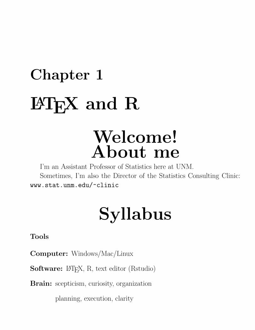
Rstudio

Quick tour

Learning the keyboard shortcuts will make your life more wonderful.

(Under Help menu)

Introduction to RR building blocks

R as calculator# Arithmetic

2 * 10

## [1] 20

1 + 2

## [1] 3

# Order of operations is preserved

1 + 5 * 10

## [1] 51

(1 + 5) * 10

## [1] 60

# Exponents use the ^ symbol

2 ^ 5

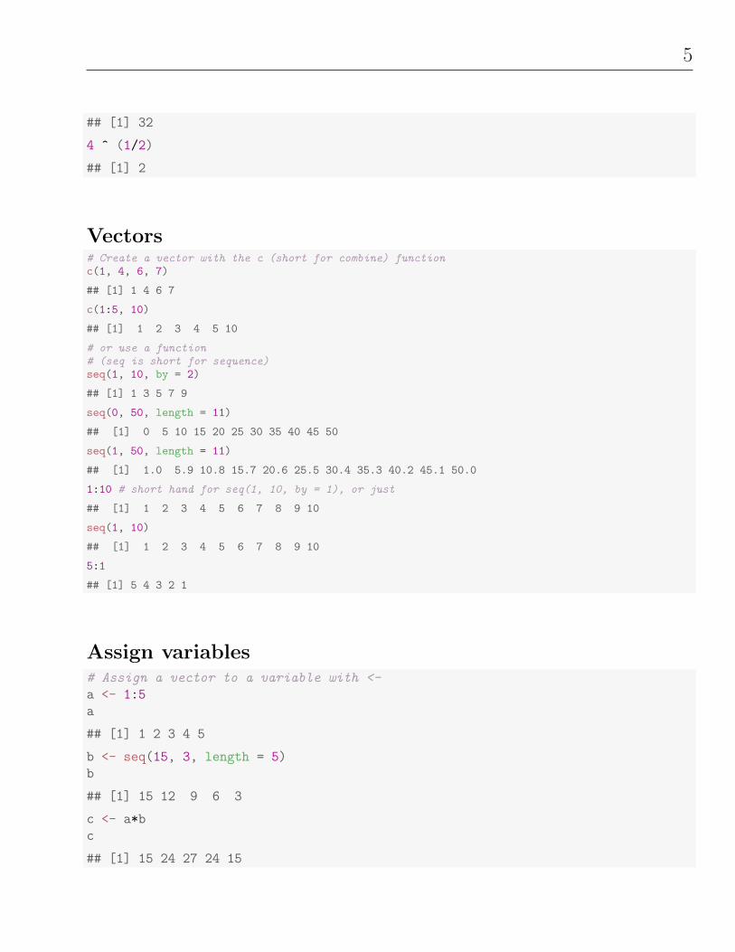
5

## [1] 32

4 ^ (1/2)

## [1] 2

Vectors# Create a vector with the c (short for combine) functionc(1, 4, 6, 7)

## [1] 1 4 6 7

c(1:5, 10)

## [1] 1 2 3 4 5 10

# or use a function# (seq is short for sequence)seq(1, 10, by = 2)

## [1] 1 3 5 7 9

seq(0, 50, length = 11)

## [1] 0 5 10 15 20 25 30 35 40 45 50

seq(1, 50, length = 11)

## [1] 1.0 5.9 10.8 15.7 20.6 25.5 30.4 35.3 40.2 45.1 50.0

1:10 # short hand for seq(1, 10, by = 1), or just

## [1] 1 2 3 4 5 6 7 8 9 10

seq(1, 10)

## [1] 1 2 3 4 5 6 7 8 9 10

5:1

## [1] 5 4 3 2 1

Assign variables# Assign a vector to a variable with <-

a <- 1:5

a

## [1] 1 2 3 4 5

b <- seq(15, 3, length = 5)

b

## [1] 15 12 9 6 3

c <- a*b

c

## [1] 15 24 27 24 15

6 LATEX and R

Basic functions# Lots of familiar functions worka

## [1] 1 2 3 4 5

sum(a)

## [1] 15

prod(a)

## [1] 120

mean(a)

## [1] 3

sd(a)

## [1] 1.581139

var(a)

## [1] 2.5

min(a)

## [1] 1

median(a)

## [1] 3

max(a)

## [1] 5

range(a)

## [1] 1 5

Extracting subsets# Specify the indices you want in the square brackets []a <- seq(0, 100, by = 10)# blank = include alla

## [1] 0 10 20 30 40 50 60 70 80 90 100

a[]

## [1] 0 10 20 30 40 50 60 70 80 90 100

# integer +=include, 0=include none, -=excludea[5]

## [1] 40

a[c(2, 4, 6, 8)]

## [1] 10 30 50 70

a[0]

## numeric(0)

a[-c(2, 4, 6, 8)]

## [1] 0 20 40 60 80 90 100

7

a[c(1, 1, 1, 6, 6, 9)] # subsets can be bigger

## [1] 0 0 0 50 50 80

a[c(1,2)] <- c(333, 555) # update a subseta

## [1] 333 555 20 30 40 50 60 70 80 90 100

True/Falsea

## [1] 333 555 20 30 40 50 60 70 80 90 100

(a > 50)

## [1] TRUE TRUE FALSE FALSE FALSE FALSE TRUE TRUE TRUE TRUE TRUE

a[(a > 50)]

## [1] 333 555 60 70 80 90 100

!(a > 50) # ! negates (flips) TRUE/FALSE values

## [1] FALSE FALSE TRUE TRUE TRUE TRUE FALSE FALSE FALSE FALSE FALSE

a[!(a > 50)]

## [1] 20 30 40 50

Comparison functions# < > <= >= != == %in%a

## [1] 333 555 20 30 40 50 60 70 80 90 100

# equal toa[(a == 50)]

## [1] 50

# equal toa[(a == 55)]

## numeric(0)

# not equal toa[(a != 50)]

## [1] 333 555 20 30 40 60 70 80 90 100

# greater thana[(a > 50)]

## [1] 333 555 60 70 80 90 100

# less thana[(a < 50)]

## [1] 20 30 40

# less than or equal toa[(a <= 50)]

## [1] 20 30 40 50

8 LATEX and R

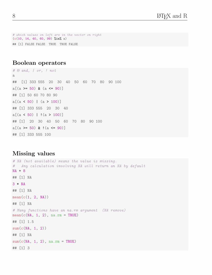
# which values on left are in the vector on right(c(10, 14, 40, 60, 99) %in% a)

## [1] FALSE FALSE TRUE TRUE FALSE

Boolean operators# & and, | or, ! not

a

## [1] 333 555 20 30 40 50 60 70 80 90 100

a[(a >= 50) & (a <= 90)]

## [1] 50 60 70 80 90

a[(a < 50) | (a > 100)]

## [1] 333 555 20 30 40

a[(a < 50) | !(a > 100)]

## [1] 20 30 40 50 60 70 80 90 100

a[(a >= 50) & !(a <= 90)]

## [1] 333 555 100

Missing values# NA (not available) means the value is missing.

# Any calculation involving NA will return an NA by default

NA + 8

## [1] NA

3 * NA

## [1] NA

mean(c(1, 2, NA))

## [1] NA

# Many functions have an na.rm argument (NA remove)

mean(c(NA, 1, 2), na.rm = TRUE)

## [1] 1.5

sum(c(NA, 1, 2))

## [1] NA

sum(c(NA, 1, 2), na.rm = TRUE)

## [1] 3

9

Missing values# Or you can remove them yourself

a <- c(NA, 1:5, NA)

a

## [1] NA 1 2 3 4 5 NA

a[!is.na(a)]

## [1] 1 2 3 4 5

a

## [1] NA 1 2 3 4 5 NA

# To save the results of removing the NAs, reassign

# write over variable a and the

# previous version is gone forever!

a <- a[!is.na(a)]

a

## [1] 1 2 3 4 5

Ch 0, R building blocks

Q1What value will R return for z?

x <- 3:7

y <- x[c(1, 2)] + x[-c(1:3)]

z <- prod(y)

z

A 99

B 20

C 91

D 54

E NA

10 LATEX and R

R building blocks 1

Answerx <- 3:7

x

## [1] 3 4 5 6 7

x[c(1, 2)]

## [1] 3 4

x[-c(1:3)]

## [1] 6 7

y <- x[c(1, 2)] + x[-c(1:3)]

y

## [1] 9 11

z <- prod(y)

z

## [1] 99

Ch 0, R building blocks

Q2What value will R return for z?

x <- seq(-3, 3, by = 2)

a <- x[(x > 0)]

b <- x[(x < 0)]

z <- a[1] - b[2]

z

A −2

B 0

C 1

D 2

E 6

11

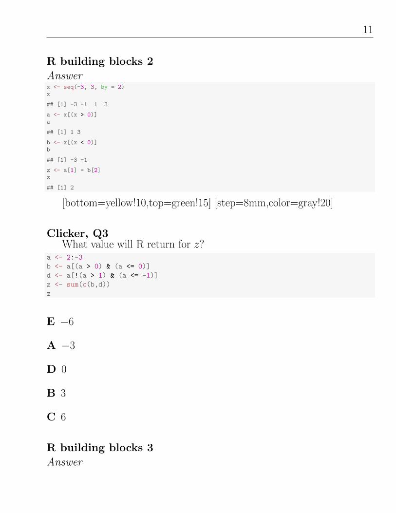
R building blocks 2

Answerx <- seq(-3, 3, by = 2)x

## [1] -3 -1 1 3

a <- x[(x > 0)]a

## [1] 1 3

b <- x[(x < 0)]b

## [1] -3 -1

z <- a[1] - b[2]z

## [1] 2

[bottom=yellow!10,top=green!15] [step=8mm,color=gray!20]

Clicker, Q3What value will R return for z?

a <- 2:-3

b <- a[(a > 0) & (a <= 0)]

d <- a[!(a > 1) & (a <= -1)]

z <- sum(c(b,d))

z

E −6

A −3

D 0

B 3

C 6

R building blocks 3

Answer

12 LATEX and R

a <- 2:-3a

## [1] 2 1 0 -1 -2 -3

a[(a > 0)]

## [1] 2 1

a[(a <= 0)]

## [1] 0 -1 -2 -3

b <- a[(a > 0) & (a <= 0)]b

## integer(0)

a[!(a > 1)]

## [1] 1 0 -1 -2 -3

a[(a <= -1)]

## [1] -1 -2 -3

d <- a[!(a > 1) & (a <= -1)]d

## [1] -1 -2 -3

z <- sum(c(b,d))z

## [1] -6

How’d you do?

Outstanding Understanding the operations and how to put them to-

gether, without skipping steps.

Good Understanding most of the small steps, missed a couple details.

Hang in there Understanding some of the concepts but all the symbols

make my eyes spin.

Reading and writing a new language takes work.

You’ll get better as you practice.

Having a buddy to work with will help.

Summary

R commands

13

# <-

# + - * / ^

# c()

# seq() # by=, length=

# sum(), prod(), mean(), sd(), var(),

# min(), median(), max(), range()

# a[]

# (a > 1), ==, !=, >, <, >=, <=, %in%

# &, |, !

# NA, mean(a, na.rm = TRUE), !is.na()

Your turn

How’s it going so far?

Muddy Any “muddy” points — anything that doesn’t make sense yet?

Thumbs up Anything you really enjoyed or feel excited about?

LATEXLATEX is a high-quality typesetting system; it includes features designed

for the production of technical and scientific documentation. LATEX is

the de facto standard for the communication and publication of scientific

documents. LATEX is available as free software.

http://www.latex-project.org/

All files are plain text files. Images of many formats can be included.

14 LATEX and R

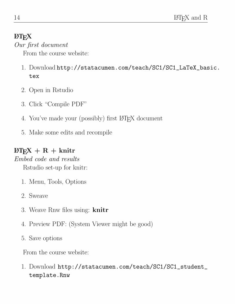
LATEX

Our first document

From the course website:

1. Download http://statacumen.com/teach/SC1/SC1_LaTeX_basic.

tex

2. Open in Rstudio

3. Click “Compile PDF”

4. You’ve made your (possibly) first LATEX document

5. Make some edits and recompile

LATEX + R + knitr

Embed code and results

Rstudio set-up for knitr:

1. Menu, Tools, Options

2. Sweave

3. Weave Rnw files using: knitr

4. Preview PDF: (System Viewer might be good)

5. Save options

From the course website:

1. Download http://statacumen.com/teach/SC1/SC1_student_

template.Rnw

15

2. Open in Rstudio

3. Click “Compile PDF”

4. Look carefully at the Rnw (R new web) source and pdf output

5. Make some edits and recompile

� See the LATEX resources on the course website.

� Practice.

� When you have errors, become good at reading the log file (with

respect to the generated .tex file line numbers).

� Can’t find the errors? Comment big chunks of code until no errors,

then uncomment small chunks until you see the error. Fix it.

For next time

� Step 0 for Thursday

� Set up LATEX + R + Rstudio

� Homework: read the introductions to LATEX and R

� Read the rubric http://statacumen.com/teach/rubrics.pdf

� If you have a disability requiring accommodation, please see me and

register with the UNM Accessibility Resource Center.