Lecture Notes Compression Technologies and Multimedia Data Formats Ao.Univ.-Prof. Dr. Andreas Uhl Department of Computer Sciences University of Salzburg Adress : Andreas Uhl Department of Computer Sciences J.-Haringerstr.2 A-5020 Salzburg ¨ Osterreich Tel.: ++43/(0)662/8044/6303 Fax: ++43/(0)662/8044/172 E-mail: [email protected]

Welcome message from author
This document is posted to help you gain knowledge. Please leave a comment to let me know what you think about it! Share it to your friends and learn new things together.
Transcript

Lecture Notes
Compression Technologies and Multimedia Data Formats
Ao.Univ.-Prof. Dr. Andreas Uhl
Department of Computer Sciences
University of Salzburg
Adress:
Andreas UhlDepartment of Computer SciencesJ.-Haringerstr.2A-5020 SalzburgOsterreichTel.: ++43/(0)662/8044/6303Fax: ++43/(0)662/8044/172E-mail: [email protected]

Inhaltsverzeichnis
1 Basics 1
1.1 What is Compression Technology ? . . . . . . . . . . . . . . . . . . . . . . . . . . . . . . . . . 1
1.2 Why do we still need compression ? . . . . . . . . . . . . . . . . . . . . . . . . . . . . . . . . 2
1.3 Why is it possible to compress data ? . . . . . . . . . . . . . . . . . . . . . . . . . . . . . . . 2
1.4 History of compression technologies . . . . . . . . . . . . . . . . . . . . . . . . . . . . . . . . . 3
1.5 Selection criteria for chosing a compression scheme . . . . . . . . . . . . . . . . . . . . . . . . 4
2 Fundamental Building Blocks 6
2.1 Lossless Compression . . . . . . . . . . . . . . . . . . . . . . . . . . . . . . . . . . . . . . . . . 6
2.1.1 Influence of the Sampling Rate on Compression . . . . . . . . . . . . . . . . . . . . . . 7
2.1.2 Predictive Coding - Differential Coding . . . . . . . . . . . . . . . . . . . . . . . . . . 7
2.1.3 Runlength Coding . . . . . . . . . . . . . . . . . . . . . . . . . . . . . . . . . . . . . . 8
2.1.4 Variable length Coding and Shannon-Fano Coding . . . . . . . . . . . . . . . . . . . . 8
2.1.5 Huffman Coding . . . . . . . . . . . . . . . . . . . . . . . . . . . . . . . . . . . . . . . 10
2.1.6 Arithmetic Coding . . . . . . . . . . . . . . . . . . . . . . . . . . . . . . . . . . . . . . 11
2.1.7 Dictionary Compression . . . . . . . . . . . . . . . . . . . . . . . . . . . . . . . . . . . 13
2.1.8 Which lossless algorithm is most suited for a given application ? . . . . . . . . . . . . 14
2.2 Lossy Compression . . . . . . . . . . . . . . . . . . . . . . . . . . . . . . . . . . . . . . . . . . 15
2.2.1 Quantisation . . . . . . . . . . . . . . . . . . . . . . . . . . . . . . . . . . . . . . . . . 16
2.2.2 DPCM . . . . . . . . . . . . . . . . . . . . . . . . . . . . . . . . . . . . . . . . . . . . . 17
2.2.3 Transform Coding . . . . . . . . . . . . . . . . . . . . . . . . . . . . . . . . . . . . . . 17
2.2.4 Codebook-based Compression . . . . . . . . . . . . . . . . . . . . . . . . . . . . . . . . 20
3 Image Compression 21
1

INHALTSVERZEICHNIS 2
3.1 Lossless Image Compression . . . . . . . . . . . . . . . . . . . . . . . . . . . . . . . . . . . . . 22
3.1.1 Fax Compression . . . . . . . . . . . . . . . . . . . . . . . . . . . . . . . . . . . . . . . 22
3.1.2 JBIG-1 . . . . . . . . . . . . . . . . . . . . . . . . . . . . . . . . . . . . . . . . . . . . 23
3.1.3 JBIG-2 . . . . . . . . . . . . . . . . . . . . . . . . . . . . . . . . . . . . . . . . . . . . 26
3.1.4 Compression of Grayscale Images with JBIG . . . . . . . . . . . . . . . . . . . . . . . 29
3.1.5 Lossless JPEG . . . . . . . . . . . . . . . . . . . . . . . . . . . . . . . . . . . . . . . . 30
3.1.6 JPEG-LS . . . . . . . . . . . . . . . . . . . . . . . . . . . . . . . . . . . . . . . . . . . 31
3.1.7 GIF, PNG, TIFF . . . . . . . . . . . . . . . . . . . . . . . . . . . . . . . . . . . . . . . 32
3.2 Lossy Image Compression . . . . . . . . . . . . . . . . . . . . . . . . . . . . . . . . . . . . . . 33
3.2.1 JPEG . . . . . . . . . . . . . . . . . . . . . . . . . . . . . . . . . . . . . . . . . . . . . 33
3.2.2 Wavelet-based Image Compression . . . . . . . . . . . . . . . . . . . . . . . . . . . . . 41
3.2.3 JPEG XR – Microsoft HD Photo . . . . . . . . . . . . . . . . . . . . . . . . . . . . . . 61
3.2.4 Fractal Image Compression . . . . . . . . . . . . . . . . . . . . . . . . . . . . . . . . . 67
3.2.5 Vector Quantization for Image Compression . . . . . . . . . . . . . . . . . . . . . . . . 74
3.2.6 Block Truncation Coding . . . . . . . . . . . . . . . . . . . . . . . . . . . . . . . . . . 76
4 Video Compression 77
4.1 Motion JPEG and Motion JPEG2000 . . . . . . . . . . . . . . . . . . . . . . . . . . . . . . . 78
4.2 MPEG-1 . . . . . . . . . . . . . . . . . . . . . . . . . . . . . . . . . . . . . . . . . . . . . . . . 78
4.3 H.261 and H.263 . . . . . . . . . . . . . . . . . . . . . . . . . . . . . . . . . . . . . . . . . . . 87
4.4 MPEG-2 . . . . . . . . . . . . . . . . . . . . . . . . . . . . . . . . . . . . . . . . . . . . . . . . 88
4.5 MPEG-4 . . . . . . . . . . . . . . . . . . . . . . . . . . . . . . . . . . . . . . . . . . . . . . . . 95
4.5.1 Compression of synthetic video objects . . . . . . . . . . . . . . . . . . . . . . . . . . . 97
4.5.2 Compression of natural video objects . . . . . . . . . . . . . . . . . . . . . . . . . . . . 98
4.6 H.264 / MPEG-4 AVC . . . . . . . . . . . . . . . . . . . . . . . . . . . . . . . . . . . . . . . . 102
4.6.1 NAL . . . . . . . . . . . . . . . . . . . . . . . . . . . . . . . . . . . . . . . . . . . . . . 102
4.6.2 VCL . . . . . . . . . . . . . . . . . . . . . . . . . . . . . . . . . . . . . . . . . . . . . . 103
4.7 Scalable Video Coding . . . . . . . . . . . . . . . . . . . . . . . . . . . . . . . . . . . . . . . . 108
4.7.1 H.264 SVC . . . . . . . . . . . . . . . . . . . . . . . . . . . . . . . . . . . . . . . . . . 109
4.7.2 3D Scalable Wavelet Video Coding . . . . . . . . . . . . . . . . . . . . . . . . . . . . . 114
4.8 Non-standard Video Coding . . . . . . . . . . . . . . . . . . . . . . . . . . . . . . . . . . . . . 117

INHALTSVERZEICHNIS 3
4.8.1 Distributed Video Coding . . . . . . . . . . . . . . . . . . . . . . . . . . . . . . . . . . 117
5 Audio Coding 120

Kapitel 1
Basics
1.1 What is Compression Technology ?
Compression denotes compact representation of data. In this lecture we exclusively cover compression ofdigital data. Examples for the kind of data you typically want to compress are e.g.
• text
• source-code
• arbitrary files
• images
• video
• audio data
• speech
Obviously these data are fairly different in terms of data volume, data structure, intended usage etc. Forthat reason it is plausible to develop specific compression technologies for different data and application ty-pes, respectively. The idea of a general purpose compression technique for all thinkable application scenarioshas to be entirely abandoned. Instead, we find a large number of very different techniques with respect totarget data types and target application environments (e.g. data transmission in networks like streaming,storage and long term archiving applications, interactive multimedia applications like gaming etc.). Giventhis vast amount of different techniques, there are different ways how to classify compression techniques:
• with respect to the type of data to be compressed
• with respect to the target application area
• with respect the the fundamental building blocks of the algorithms used
1

KAPITEL 1. BASICS 2
Terminology: when talking abount compression, we often mean “lossy compression” while “lossless com-pression” is often termed as coding. However, not all coding algorithm do actually lead to lossless compres-sion, e.g. error correction codes. Like in every other field in computer science or engineering, the dominatinglanguage in compression technologies is English of course. There are hardly any comprehensive and up-to-date German books available, and there do NOT exist any German journals in the field. Codec denotesa complete system capable of encoding and decoding data which consists of an Encoder and a Decoder,transcoding is a conversion from one encoded digital representation into another one. A fundamental termin the area is compression rate (or compression ratio) which denotes the relation between the size of theoriginal data before compression and the size of the compressed data. Compression ratio therefore rates theeffectivity of a compression system in terms of data reduction capability. This must not be confused withother measures of compressed data size like bit per pixel (bpp) or bit per sample (bps).
1.2 Why do we still need compression ?
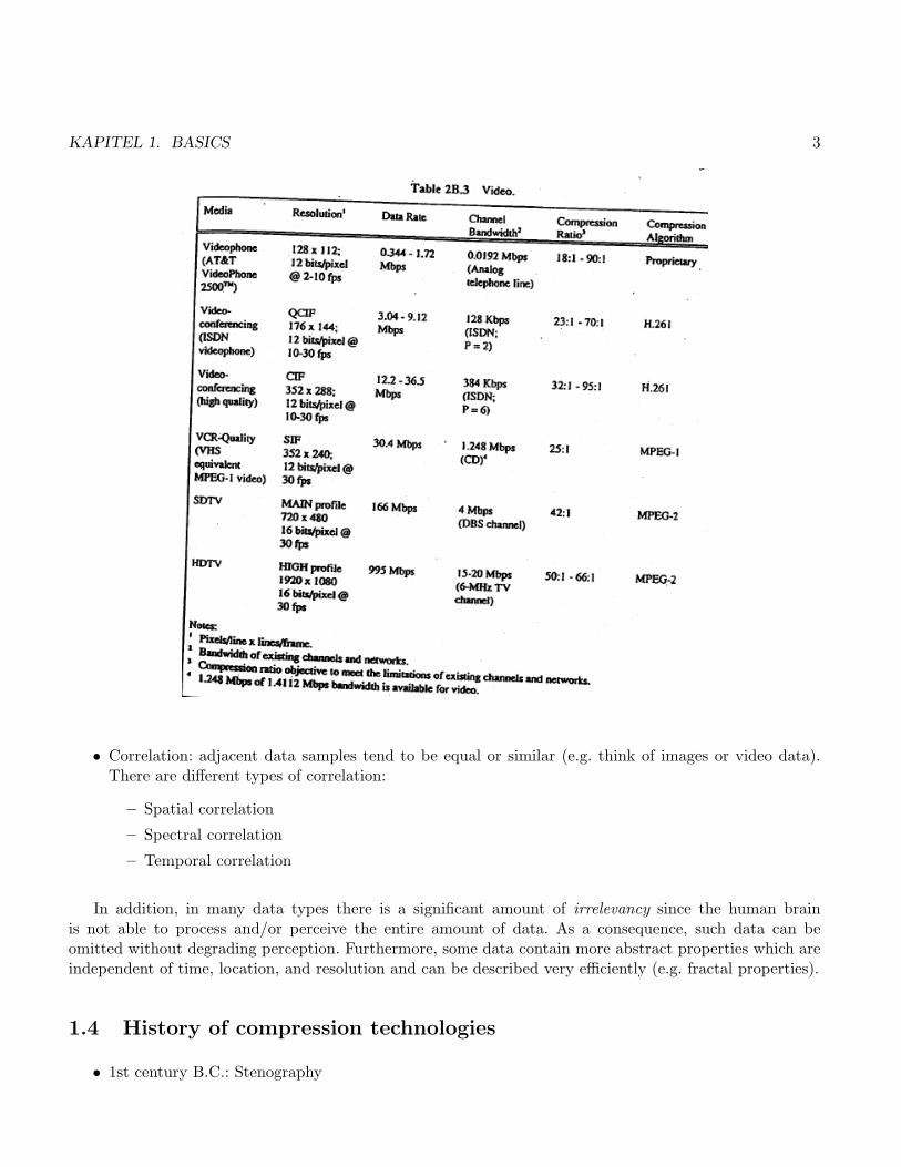
Compression Technology is employed to efficiently use storage space, to save on transmission capacity andtransmission time, respectively. Basically, its all about saving resources and money. Despite of the overwhel-ming advances in the areas of storage media and transmission networks it is actually quite a surprise thatstill compression technology is required. One important reason is that also the resolution and amount ofdigital data has increased (e.g. HD-TV resolution, ever-increasing sensor sizes in consumer cameras), andthat there are still application areas where resources are limited, e.g. wireless networks. Apart from the aimof simply reducing the amount of data, standards like MPEG-4, MPEG-7, and MPEG-21 offer additionalfunctionalities.
During the last years three important trends have contributed to the fact that nowadays compressiontechnology is as important as it has never been before – this development has already changed the way wework with multimedial data like text, speech, audio, images, and video which will lead to new products andapplications:
• The availability of highly effective methods for compressing various types of data.
• The availability of fast and cheap hardware components to conduct compression on single-chip systems,microprocessors, DSPs and VLSI systems.
• Convergence of computer, communication, consumer electronics, publishing, and entertainment indu-stries.
1.3 Why is it possible to compress data ?
Compression is enabled by statistical and other properties of most data types, however, data types existwhich cannot be compressed, e.g. various kinds of noise or encrypted data. Compression-enabling propertiesare:
• Statistical redundancy: in non-compressed data, all symbols are represented with the same number ofbits independent of their relative frequency (fixed length representation).
KAPITEL 1. BASICS 3
• Correlation: adjacent data samples tend to be equal or similar (e.g. think of images or video data).There are different types of correlation:
– Spatial correlation
– Spectral correlation
– Temporal correlation
In addition, in many data types there is a significant amount of irrelevancy since the human brainis not able to process and/or perceive the entire amount of data. As a consequence, such data can beomitted without degrading perception. Furthermore, some data contain more abstract properties which areindependent of time, location, and resolution and can be described very efficiently (e.g. fractal properties).
1.4 History of compression technologies
• 1st century B.C.: Stenography

KAPITEL 1. BASICS 4
• 19th century: Morse- and Braille alphabeths
• 50ies of the 20th century: compression technologies exploiting statistical redundancy are developed –bit-patterns with varying length are used to represent individual symbols according to their relativefrequency.
• 70ies: dictionary algorithms are developed – symbol sequences are mapped to shorter indices usingdictionaries.
• 70ies: with the ongiong digitization of telephone lines telecommunication companies got interested inprocedures how to get more channels on a single wire.
• early 80ies: fax transmission over analog telephone lines.
• 80ies: first applications involving digital images appear on the market, the “digital revolution” startswith compressing audio data
• 90ies: video broadcasting, video on demand, etc.
1.5 Selection criteria for chosing a compression scheme
If it is evident that in an application compression technology is required it has to be decided which typeof technology should be employed. Even if it is not evident at first sight, compression may lead to certainsurprising benefits and can offer additional functionalities due to saved resources. When selecting a specificsystem, quite often we are not entirely free to chose due to standards or de-facto standards – due tothe increasing develeopment of open systems and the eventual declining importance of standards (example:MPEG-4 standardization !) these criteria might gain even more importance in the future. Important selectioncriteria are for example:
• data dimensionality: 1-D, 2-D, 3-D, .........
• lossy or lossless compression: dependent of data type, required quality, compression rate
• quality: with target quality is required for my target application ?
• algorithm complexity, speed, delay: on- or off-line application, real-time requirements
• hardware or software solution: speed vs. price (video encoder boards are still costly)
• encoder / decoder symmetry: repeated encoding (e.g. video conferencing) vs. encoding only once butdecoding often (image databases, DVD, VoD, ....)
• error robustness and error resilience: do we expect storage or transmission errors
• scalability: is it possible to decode in different qualities / resolutions without hassle ?
• progressive transmission: the more data we transmit, the better the quality gets.

KAPITEL 1. BASICS 5
• standard required: do we build a closed system which is not intended to interact with other systems(which can be desired due to market position, e.g. medical imaging) or do we want to exchange dataacross many systems
• multiple encoding / decoding: repeated application of lossy compression, e.g. in video editing
• adaptivity: do we expect data with highly varying properties or can we pre-adapt to specific properties(fingerprint compression)
• synchronisation issues – audio and video data should both be frame-based preferably
• transcoding: can the data be converted into other datatypes easisly (e.g. MJPEG −− > MPEG)

Kapitel 2
Fundamental Building Blocks
2.1 Lossless Compression
In lossless compression (as the name suggests) data are reconstructed after compression without errors,i.e. no information is lost. Typical application domains where you do not want to loose information iscompression of text, files, fax. In case of image data, for medical imaging or the compression of maps in thecontext of land registry no information loss can be tolerated. A further reason to stick to lossless codingschemes instead of lossy ones is their lower computational demand. For all lossless compression techniquesthere is a well known trade-off: Compression Ratio – Coder Complexity – Coder Delay.
Lossless Compression typically is a process with three stages:
• The model: the data to be compressed is analysed with respect to its structure and the relativefrequency of the occuring symbols.
• The encoder: produces a compressed bitstream / file using the information provided by the model.
• The adaptor: uses informations extracted from the data (usually during encoding) in order to adaptthe model (more or less) contineously to the data.
The most fundamental idea in lossless compression is to employ codewords which are shorter (in termsof their binary representation) than their corresponing symbols in case the symbols do occur frequently.On the other hand, codewords are longer than the corresponding symbols in case the latter do not occurfrequently (there’s no free lunch !).
Each process which generates information can be thought of a source emitting a sequence of symbolschosen from a finite alphabeth (in case of computer-based processing this boils down to the binary alphabeth0,1). We denote this “source of information” by S with the corresponding alphabeth {s1, s2, . . . , sn} andtheir occurance probabilities {p(s1), p(s2), . . . , p(sn)}. To make things simpler (and more realistic as well),we consider these probabilities as being relative frequencies. We want to determine the average informationa source emits. Following intuition, the occurence of a less frequent symbol should provide more informationcompared to the occurence of highly frequent symbols. We assume symbols to be independent and considerthe information provided by such symbols as being the sum of information as given by the single independent
6

KAPITEL 2. FUNDAMENTAL BUILDING BLOCKS 7
symbols. We define
I(si) = log1
p(si)
as being the information delivered by the occurence of the symbol si related to its probability p(si). Thebasis of the logarithm determines the measure of the amount of information, e.g. in case of basis 2 we talkabout bits.
By averaging over all symbols emitted by the source we obtain the average information per symbol, theentropy:
H(S) =n∑
i=1
p(si)I(si) = −n∑
i=1
p(si) log2 p(si) bits/symbol
The most significant interpretation of entropy in the context of lossless compression is that entropymeasures how many bits are required on average per symbol in order to represent the source, i.e. to conductlossless compression. Entropy therefore gives a lower bound on the number of bits required to represent thesource information. In the next section we will discuss several techniques approaching more or less closelythis theoretical bound.
2.1.1 Influence of the Sampling Rate on Compression
If we compare data originating from an identical analog source where yi is sampled ten times as densly asxi, we notice that neighbouring values of yi tend to be much more similar as compared to neighbouringvalues in xi. If we assume that the analog signal exhibits continuity to some degree, the samples of yi willbe more contineous (i.e. more similar) as compared to the samples of xi since these are taken from locationsin the signal more dislocated as the samples of yi. The higher degree of similarity in yi has a positive effecton entropy and therefore on the achievable compression ratio.
2.1.2 Predictive Coding - Differential Coding
This technique is not really a compression scheme but a procedure to preprocess data in order to make themmore suited for subsequent compression. Differential coding changes the statistics of the signal – based onthe fact that neighbouring samples in digital data are often similar or highly correlated, differential codingdoes not compress the sequence of original data points {x1, x2, . . . , xN} but the sequence of differencesyi = xi − xi−1. While xi usually follow a uniform or normal distribution, yi exhibit significant peaks around0 (always assuming that neighbouring samples tend to be similar as it is the case in audio, image, and videodata). To give an example, we consider an image with 999 pixels and 10 different symbols. In case a) wehave p(si) = 1/10, i = 1, . . . , 10, in case b) we have p(s1) = 91/100 and p(si) = 1/100 for i = 2, . . . , 10.Case a) corresponds to the “conventional” image with unifomly distributed symbols, while case b) is thedifferential image consisting of yi, where s1 is the zero symbol. In case a) we result in H(S) = 3.32, while incase b) entropy is only H(S) = 0.72. This small example immediately makes clear that differential codingis sensible. Actually, it is the basis of many compression schemes employing prediction.

KAPITEL 2. FUNDAMENTAL BUILDING BLOCKS 8
2.1.3 Runlength Coding
The basic principle is to replace sequences of successive identical symbols by three elements: a single symbol,a counter, and an indicator which gives the interpretation of the other two elements.
As an example we discuss the tape drive of the IBM AS/400 (where obviously lots of blanks are en-countered): strings of consecutive blanks (2-63 byte) are compressed into a codeword which contains theinformation “blank” and a counter. Strings of consecutive identical characters unequal blank (3-63 byte)are compressed into 2 byte: Control byte (“connsecutive char” and counter) and character byte. Strings ofnon-consecutive identical characters are expanded by a control byte (“non- consecutive identical”).
Example: b Blank, * control byte; bbbbbbABCDEFbb33GHJKbMN333333 is compressed into **ABC-DEF**33GHJKbMN*3
ATTENTION: if the data is not suited for runlength encoding we result in data expansion (caused bythe expansion of non-consecuritve identical chars). Runlengh coding is extremely fast on the other hand andcan compress quite well in case of suited data.
2.1.4 Variable length Coding and Shannon-Fano Coding
We denote the length of the codeword for the symbol si as l(si) (in bits). The average code length is definedas: L(S) =
∑ni=1 p(si)l(si). In order to minimize this expression (which obviously is the aim of compression)
we need to assign short codewords to symbols with high probability of occurence. It is intersting to noticethe close relation to entropy: H(S) =
∑ni=1 p(si)I(si). Consequently it is evendent that l(si) = I(si) =
− log2 p(si) needs to be fulfilled in order to attain the actual entropy value. However, this is possible onlyin case log2 p(si) is a natural number. Usually, this is not the case of course, so the value is rounded to thenext integer (which is a hint to the sub-optimality of the entire procedure !). Shannon-Fano Coding (seebelow) exactly provides the corresponding solution using the idea described before. The term code efficiencyis defined as H(S)
L(S) – obviously values close to 1 are desirable !

KAPITEL 2. FUNDAMENTAL BUILDING BLOCKS 9
Example: S = {s1, s2, s3, s4} with p(s1) = 0.6, p(s2) = 0.3, p(s3) = 0.05 and p(s4) = 0.05. H(S) = 1.4bits/symbol. When chosing a fixed length encoding like e.g. 00, 01, 10, 11 as codewords with average codelength of 2 bits/symbol. When computing l(si) we obtain the values 1,2, and 5 and result in the followingvariable length code: 0, 10, 110 und 111. s3 and s4 would require a 5 bit codeword but 3 bits are sufficientto generate a unique code. The corresponding average code length is 1.5 bits/symbol.
A prefix code (or prefix-free code) is a code system, typically a variable-length code, with the “prefixproperty”: there is no valid code word in the system that is a prefix (start) of any other valid code word inthe set. E.g., a code with code words 9, 59, 55 has the prefix property; a code consisting of 9, 5, 59, 55 doesnot, because 5 is a prefix of both 59 and 55. With a prefix code, a receiver can identify each word withoutrequiring a special marker between words.
A way to generate a prefix code is to use a full binary tree to represent the code. The leaves represent thesymbols to be coded while path traversing the tree from the root to the leave determines the bit-sequence ofthe resulting codeword. To actually determine a bitsequence, we need to define how to encode a branching:for example, a branching to the left can be encoded by 0 and a branching to the right by 1. The tree givenin the figure leads to the following codewords: A – 00, B – 01, C – 100, D – 101, E – 1. The tree (and code)generation of the Shannon-Fano scheme works as follows (in the example, we assume the following frequencycounts: A – 15, B – 7, C – 6, D – 6, E – 5):
1. For a given list of symbols, develop a corresponding list of probabilities or frequency counts so thateach symbol’s relative frequency of occurrence is known.
2. Sort the lists of symbols according to frequency, with the most frequently occurring symbols at theleft and the least common at the right.
3. Divide the list into two parts, with the total frequency counts of the left half being as close to thetotal of the right as possible.
4. The left half of the list is assigned the binary digit 0, and the right half is assigned the digit 1. Thismeans that the codes for the symbols in the first half will all start with 0, and the codes in the secondhalf will all start with 1.

KAPITEL 2. FUNDAMENTAL BUILDING BLOCKS 10
5. Recursively apply the steps 3 and 4 to each of the two halves, subdividing groups and adding bits tothe codes until each symbol has become a corresponding code leaf on the tree.
A procedure often employed is to replace the alphabeth consisting of the si by an extension using tuplessisj with their corresponding relative frequencies. Using this strategy, a code length of 1.43 bits/symbol canbe achieved, however, at a higher cost in terms of computation and memory requirements.
2.1.5 Huffman Coding
Huffman Coding is a popular technique using the idea of variable length coding combined with a constructivealgorithm how to build the corresponding unique codewords. Suppose we have given a source S with analphabeth of size n. The two least frequent symbols are combined into a new virtual symbol which isassigned the sum of occurence probabilites of the two original symbols. Subsequently, the new alphabeth ofsize n− 1 is treated the same way, which goes on until only two symbols are left. If we know the codewordsof the new symbols, the codewords for the two original symbols are obtained by adding a 0 and 1 bit tothe right side of the new symbol. This procedure is applied recursively, i.e. starting with the two mostfrequent symbols which are assigned codewords 0 and 1, we successively add corresponding bits to the rightuntil codewords for all original symbols have been generated. The example has entropy H(S) = 2.15, thegererated Huffman code have average code length of 2.2 bits/symbol, an ad-hoc generated code like shownbefore, like e.g. {0, 10, 110, 1110, 1111} has average code length of 2.25 bits/symbol.
Modification: in case many symols have small probabilities of occurence, a large number of long codewordsis the result which is not efficient. Therefore, all such symbols are assinged into a dedicated class which istermed “ELSE” in the Huffman code and which is encoded separately. This idea is calles modified Huffmancode.
Problems:
1. In case a source has a symbol with p(s) close to 1 and many others with small probability of occurencewe result in an average code length of 1 bit/symbol since the smallest length for a codeword is ofcourse 1 bit. The entropy is of course much smaller (recall the coding of differences).
2. In case of changing statistics of the source one can easily obtain a data expansion.
3. Since a fixed codebook is of poor quality in many cases we have a two stage algorithm: buildingstatistics (the model), generate the code.

KAPITEL 2. FUNDAMENTAL BUILDING BLOCKS 11
4. Adaptivity is difficult to implement, since changes in the statistics affect the entire tree and not justa local part. We can either store corresponding Huffman tables (trees) in the data [which is inefficientin terms of compression] or compute them on the fly from decoded data [which is inefficient in termsof compression speed].
Huffman encoding is used in most older standards like JPEG, MPEG-1 to MPEG-4, however, in anon-adaptive manner which is possible due to the nature of the DCT transform.
2.1.6 Arithmetic Coding
In Huffman coding we have a correspondence between a single symbol and its codeword – which is themain reason for its suboptimality. Arithmetic coding uses a single codeword for an entire sequence of sourcesymbols of length m. In this manner the restriction to integer-valued bits per symbol values can be avoidedin an elegant way. A drawback however is that similar sequences of source symbols can lead to entirelydifferent codewords.
The principal idea is as follows. Suppose we have a sequence of binary source symbols sm with lengthm where p(0) = p and p(1) = 1 − p. Let I = [0, 1) be the semi-open unit interval and
∑p(sm) = 1
when summing over all 2m possible sequences of length m. Based on this initial construction we can buildsubintervals Il with l = 1, 2, . . . , 2m which are all in I and which can be assinged in unique manner to asequence sm where |Il| = p(sm) and all Ij are disjoint. The following procedure constructs such intervalsand is called “Elias Code” (this approach is meant for illustrative purposes only since it is inpractical forimplementations).
The interval I is partitioned into two subintervals [0,p) (in case 0 is the symbol to be coded) and [p,1)(in case 1 is to be coded). Based on the occurance of the next symbol (0 or 1) these intervals are furtherpartitioned recursively into [0, p2) and [p2, p) and into [p, 2p− p2) and [2p− p2, 1), respectively. The interval[p2, p) for example is assigned to the sequence 01. After j − 1 source symbols the interval [Lj−1, Rj−1) hasbeen assigned to the sequence sj−1.
• 0 is next: Lj = Lj−1 and Rj = Lj−1 + p(Rj−1 − Lj−1).
• 1 is next: Lj = Lj−1 + p(Rj−1 − Lj−1) und Rj = Rj−1.
Based on this construction one can show that the length of each interval [Lj , Rj) has the same length asp(sm) of the corresponding sequence. As soon as the interval has been constructed, the codeword for sm isfound easily: we represent Lj in binary manner and keep − log2 p(sm) bits (rounded to next integer) afterthe decimal point. This is sufficient to uniquely identify the interval and the corresponding symbol sequence.In actual implementations it is sufficient to encode an arbitrary point in the constructed interval (of coursea point with minimal length in the binary representation is selected) and the number of encoded symbols.An important fact is that in small intervals, more binary positions are required to represent a point (sinceno points with small “binary length” are contained).
Actual implementations use a re-normalisation to [0, 1) in each interval partitioning stage due to problemswith rounding errors.
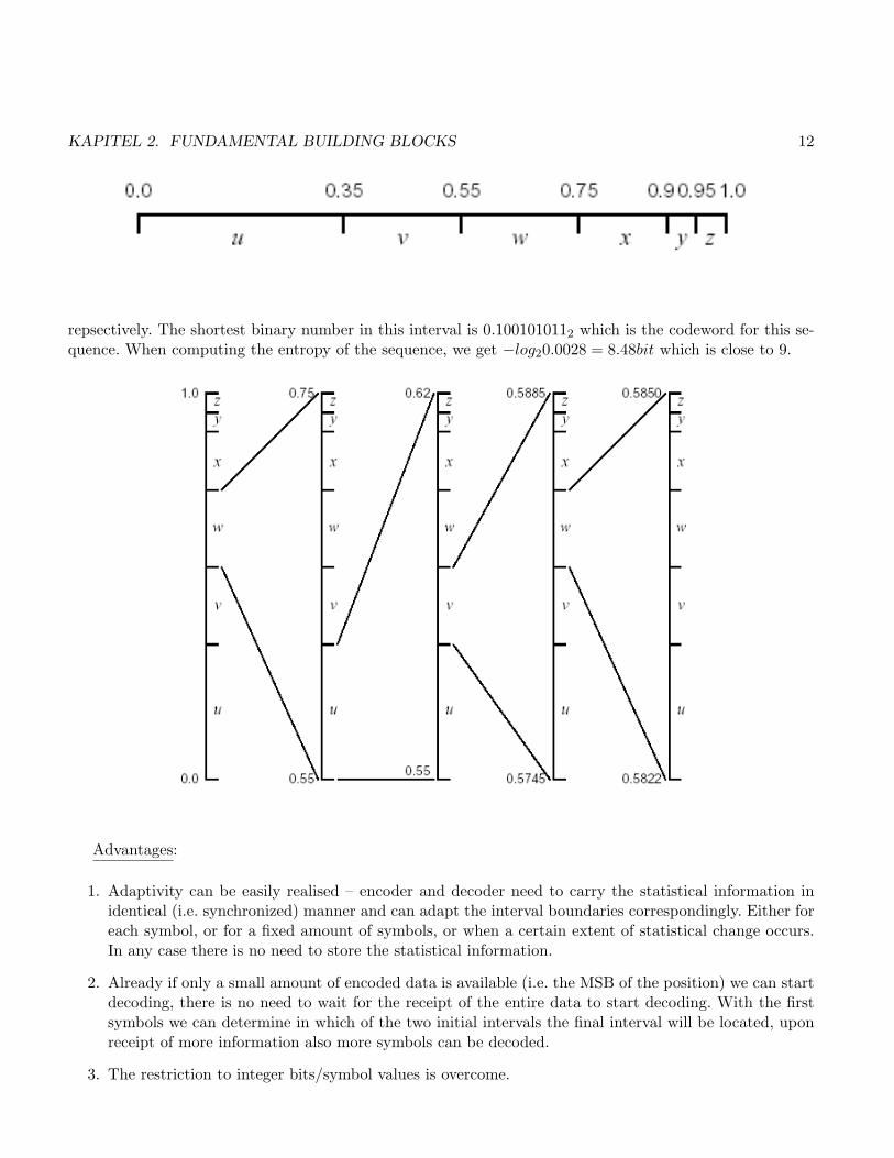
Example: Encoding the sequence wuvw leads to the interval [0.5822, 0.5850] the length of which is 0.0028= p(w)p(u)p(v)p(w). In binary representation the interval borders are 0.10010101110002 and 0.10010101000012,
KAPITEL 2. FUNDAMENTAL BUILDING BLOCKS 12
repsectively. The shortest binary number in this interval is 0.1001010112 which is the codeword for this se-quence. When computing the entropy of the sequence, we get −log20.0028 = 8.48bit which is close to 9.
Advantages:
1. Adaptivity can be easily realised – encoder and decoder need to carry the statistical information inidentical (i.e. synchronized) manner and can adapt the interval boundaries correspondingly. Either foreach symbol, or for a fixed amount of symbols, or when a certain extent of statistical change occurs.In any case there is no need to store the statistical information.
2. Already if only a small amount of encoded data is available (i.e. the MSB of the position) we can startdecoding, there is no need to wait for the receipt of the entire data to start decoding. With the firstsymbols we can determine in which of the two initial intervals the final interval will be located, uponreceipt of more information also more symbols can be decoded.
3. The restriction to integer bits/symbol values is overcome.

KAPITEL 2. FUNDAMENTAL BUILDING BLOCKS 13
Arithmetic coding is used in JBIG-1 as the only coding engine and in the more recent lossy standardslike JPEG2000 and H.264 as lossless compression stage.
2.1.7 Dictionary Compression
Basic idea: the redundancy of repeated phrases in a text is exploited (recall: in Runlenth encoding, repeatedidentical symbols can be efficiently coded). Here we encode repeatedly occuring symbol strings in arbitraryfiles in an efficient manner. A frontend selects strings and information for compression and dekompressionis stored in a dictionary. The encoder and the decoder need to have access to a copy of this dictionary ofcourse. In this manner, entire strings are replaced by tokens (i.e. codewords). The basic algorithmic elementsare lookup tables, and the corresponding operations are very fast.
LZ77 Dictionary Compression
The name originates from Lempel and Ziv (1977), the algorithm actually described here is a variant, LZSS(Storer/Szymanski) as of 1982. A typical feature is the so-called “sliding window” consisting of two parts:the history buffer (the dictionary) contains a block of data recently encoded (some 1000 symbols) – and thelook-ahead buffer which contains strings to be encoded (10-20 symbols).
In important issue is the coice of the buffer sizes:
• History buffer small − > match is unlikely.
• History buffer large − > high computational requirements and poor compression rate caused by thelarge address space for the pointers into the buffer.

KAPITEL 2. FUNDAMENTAL BUILDING BLOCKS 14
• Look-ahead buffer small − > no match for long strings is possible (waste of potential redundancy).
• Look-ahead buffer large − > time is wasted for the unlikely case of finding matches for long strings.
Example: Text out < − ——DATA COMPRESSION—— COMPRESSES DATA—— < − Text in.“DATA COMPRESSION” is the content of the history buffer, “COMPRESSES DATA” is the look-aheadbuffer. The actual coding used subsequently is the QIC-122 standard for tape drives using a history bufferof 2048 bytes.
To start with, we encode each symbol in “DATA COMPRESSION” as 0<ASCII Char. Wert>. “COM-PRESS” is a string of length 9 which has been found in the history buffer 12 symbols backwards: 1<offset=12><length=9>.Subsequently we encode “E” and “S” again as 0<ASCII Char. Wert> and “DATA” as string of length 4which has been found in the history buffer 28 positions backwards: 1<offset=28><length=4>.
We notice that
• the algorithm requires a start-up phase where the data in the dictionary has to be encoded explicitely,which means that it is hardly suited for compressing lots of small files.
• The algorithm is assymetric – searching the history buffer in an efficient manner is crucial. Intelligentdata structures are required.
• Since data leaves the history buffer after some time, long term redundancy cannot be exploited.
LZ78 Dictionary Compression
The algorithm described here the LZW(elch) Coding variant as of 1984. This algorithm solves the problemsarising with the explicit definition of the two buffers. Stings in the dictionary are not automatically reasedand the lookahead buffer does not have a fixed size. The algorithm does not employ pointers to earliercomplete strings but a procedure called “Phrasing”. A text is divided into phrases, where a phrase is thelongest string found so far plus an additional character.
All symbols are replaced by topkens (i.e. codewords) which point to entries in the dictionary. The first256 disctionary entries are the common 8 bit ASCII code symbols. The dictionary is successively extendedby new phrases generated from the text (i.e. data) to be coded.
Critical issues:
• How to efficiently encode a variable number of strings with variable length ?
• How long can we grow the dictionary ? What are the strategies when the dictionary gets too large(start from scratch, keep the most common entries) ?
2.1.8 Which lossless algorithm is most suited for a given application ?
Testing with exemplary data is important apart from the facts we know theoretically with respect to speed,assymetry, compression capability etc. !

KAPITEL 2. FUNDAMENTAL BUILDING BLOCKS 15
2.2 Lossy Compression
In addition to the tradeoff between coding efficiency – coder complexity – coding delay the additionalaspect of compression quality arises with the use of lossy methods. Quality is hard to assess since for manyapplication human perception is the only relevant criterion. However, there are some scenarios where otherfactors need to be considered, e.g. when compressed data is used in matching procedures like in biometrics.Although several quality measures have been proposed over the last years, PSNR is still the most usedmeasure to determine image and video quality after compression has been applied:
RMSE =
√√√√1/NN∑
i=1
(f(i)− f ′(i))2
where f ′(i) is the reconstructed signal after decompression. Peak-signal-to-noise ratio (measured in de-ciBel dB) is defined as follows (where MAX is the maximal possible value in the original signal f(i)):
PSNR = 20 log10(MAX
RMSE).

KAPITEL 2. FUNDAMENTAL BUILDING BLOCKS 16
The higher the value in terms of PSNR, the better is the quality of the reconstructed signal. Withincreasing compression ratio, PSNR decreases. While PSNR is not well correlated with moderate qualitychanges, it serves its purpose as a rough quality guideline. Many other numerical measures have beendeveloped with better prediction of human perception (e.g. structured similarity index SSIM) but thesehave not been widely adopted One reason is that image compression can be easily optimized with respectto RMSE (rate / distortion optimisation), but not with respect to the “better” measures. In order to reallytake human perception into account, subjective testing involving a significant number of human subjectsis necessary – the resulting subjective measure is called MOS (“mean opinion score”). When developingquality measures, a high correlation with MOS computed over large databased is desired. PSNR does notcorrelate well with MOS.
2.2.1 Quantisation
When changing the description of a signal from using a large alphabeth to using a smaller alphabeth ofsymbols we apply quantisation. Obviously, when reversing the process, a perfect reconstuction is no longerpossible since two or more symbols of the larger alphabeth are mapped to a single symbol of the smallalphabeth. Often, quantisation errors are the only actual errors caused by lossy compression (apart fromrounding errors in transforms).
Example: suppose we have stored a grayscale image with 8bit/pixel (bpp) precision, which means that foreach pixel, we may choose among 256 different grayscales. If we apply a quantisation to 4 bpp, only 16grayscale can be used for a pixel. Of course, it is no longer possible to re-transform the 4 bpp into theoriginal bit-depth without errors. The information is lost.
If single signal values are subject to quantisation one-by-one (a single value is quantised into its less accu-rate version), the procedure is denoted “scalar quantisation”. If we subject n-tuples of signal values togetherto quantisation (a vector is replaced by a less accurate version), we call the scheme “vector quantisation”.In any case, quantisation may be interpreted as a specific kind of approximation to the data.
If we devide the range of the original signal into n equally sized and disjoint intervals and map all symbolscontained in an interval to one of the n symbols of the new alphabeth, the quantisation is called “uniform”.Especially in the case of uniformly distributed probabilities of symbol occurrence uniform quantisation makessense. Quantisation is most often applied to transform coefficients (e.g. after DCT or wavelet transform) – inthis context, coefficients quantised to zero are desired to appear frequently. Therefore, “uniform quantisationwith deadzone around 0” is introduced, we uniform quantisation is applied, except for the quantisation binaround zero, which has twice the size of the other bins (symetrically around zero).
In case the occurrence probabilities of the symbols in the original signal are not uniformly distributedand the distribution is known, it makes sense to apply finer quantisation (i.e. smaller bins) in the areas of thehistogram where more data values are accumulated. In this case we talk about “non- uniform quantisation”.Note that following this strategy we minimise PSNR (the error is minimized in areas where many values arefound) but we do not care at all about perceptual issues.
If the distribution of the occurrence probabilities of the symbols is not known, the signal can be analysedand based on the results, the quantisation bins can be set adaptively – termed “adaptive quantisation”.Since especially in the case of transform coding in many cases the probabilities of symbol occurrence is quitestable for typical signals, quatisation can be modeled in advance and does not have to be adapted to signal

KAPITEL 2. FUNDAMENTAL BUILDING BLOCKS 17
characteristics.
2.2.2 DPCM
Differential pulse code modulation (DPCM) is the general principle behind differential / predictive coding.Instead of considering the simple difference between adjacent signal values, also the difference between asignal value to be predicted and a linear-combination of surrounding values (i.e. the prediction) can beconsidered.
Example: yi = xi − x′i, where x′i = αxi−1 + βxi−2 + γxi−3. The values α, β, γ are denoted “predictorcoefficients”, x′i is the prediction for xi. The example is a linear predictor of order 3. Instead of storingor processing the sequence xi, the sequence of differences yi is considered, which has a significantly lowerentropy (and can therefore be better compressed).
The predictor coefficients can be fixed for classes of known signals (e.g. exploiting specific patternslike ridges in fingerprint images) or can be adapted for each single signal (in the latter case, these needto be stored). The optimal values for α, β, γ e.g. minimising entropy for yi can be determined of course.Furthermore, for each distinct part of a signal dedicated coefficients can be used and optimsied (“localadaptive prediction”). By analogy, these coefficients need to be stored for each signal part impacting oncompression ratio (obviously, there is a trade-off !).
The decision if DPCM is lossy or lossless is taken by the way how yi is compressed. In case e.g. Huffmancoding is applied to yi we result in an overall lossless procedure. Is yi subject to quantisation, the overallscheme is a lossy one.
A variant of DPCM frequently employed is to use a fixed set of predictor and quantiser combinationswhich are applied tp the data depending on local signal statistics. Lossless JPEG is such a scheme (withoutapplying quantisation of course).
2.2.3 Transform Coding
Most standardised lossy media compression schemes are based on transform coding techniques. Typically,tranform based coding consists of three stages.
1. Transformation
2. Quantisation: a variety of techniques (as discussed before) can be applied to map the transform coef-ficients to a small alphabeth, the size of the latter being selected corresponding to the target bitrate.Most rate-control procedures are applied in this stage.
3. Lossless encoding of coefficients: a variety of techniques (as discussed before) is applied in order toencode the quantised transform coefficients close to the entropy bound. Typically, a combination ofrunlength (zero-runs !) and Huffman coding (for the older standards like JPEG, MPEG-1,2,4) orarithmetic coding (for the more recent standards like JPEG2000 H.264) is used.
KAPITEL 2. FUNDAMENTAL BUILDING BLOCKS 18
The Transform
The aim of transformation is to change the data of a signal in a way that it is better suited for subsequentcompression. In most cases, so-called “integral-transforms” are used, which are based (in their contineousform) on applying integral operators. When applying transforms, the concept of projecting the data ontoorthogonal basis functions is used.
Motivation: Vectors in two-dimensional space can be represented by a set of othogonal basis-vectors(“orthogonal basis”, orthogonal requires the inner product between vectors to be 0).
(x, y) = α(1, 0) + β(0, 1).
{(1, 0), (0, 1)} are orthogonal basis-vectors, α und β are called “coefficients” which indicate a weight for eachbasis-vector in order to be able to represent the vector (x, y). The property of orthogonality guarantees thata minimal number of basis-vectors suffices (obviously, this will be important for compression).
This concept can be transferred by analogy to represent functions or signals by means of basis elements.
f(x) =∑
n
< f(x), ψn(x) > ψn(x)
ψn(x) are orthogonal basis-functions, < f(x), ψn(x) > are transform coefficients which determine the weightto be applied to each basis-function, to represent a given signal. When performing the actual compression,the < f(x), ψn(x) > are computed, quantised, and stored in encoded form. Since ψn(x) are chosen to be anorthogonal function system, the corresonding number of coefficients to be stored is minimal.
Example: in the case of the Fourier transform ψn(x) = e−πinx = cos(nx)− i sin(nx). In this special case weobserve the frequency of periodic signals. A Fourier coefficient < f(x), ψn(x) > reports the strength of thefrequency component n in the signal which has been subjected to the transform. Obviously, not all functionscan be represented well by stationary (i.e. frequency does not change over time) periodic basis functions.This is where the wavelet transform and other types enter the scene.
To conduct transform coding, we represent the signal f(x) by f(x) =∑
n < f(x), ψn(x) > ψn(x)(i.e. the transform coefficients are computed). The transform coefficients < f(x), ψn(x) > are quantisedsubsequently and finally compressed losslessly. In case ψn(x) are well chosen, the transform coefficients are 0after quantization for most basis functions and do not need to be stored. Consequently, in the reconstructionthe error is small, since most coefficients were 0 anyway. Most of the signal information is concentrated in asmall number of coefficients – we speak of energy compactation here. Therefore, the art of transform codingis to select an appropriate set of suited basis functions that works well for a wide class of signals.
A further way to interpret integral transforms is to view them as a rotation of the coordinate axes. Thedata is transformed into a coordinate system, which allows for a more efficient compression. As a motivationfor this interpretation, we consider pairs X = (x1, x2) which are gernerated from neighboring pixel valuesin an image. Plotting all pairs into a coordinate system most of the pairs are positioned around the maindiagonal (since most neighboring pixels tend to be similar). The variance of xj is defined as
σ2xj
= 1/MM∑i=1
(xji − xj)2
where M is the number of pairs and xj is the mean of xj computed over all pairs. A simple technique toapply compression is to replace one of the two components in each pair by the corresponding mean xj. The

KAPITEL 2. FUNDAMENTAL BUILDING BLOCKS 19
MSE of this compression approach is exactly σ2xj
, the variance. No matter which coordinate we replace bethe mean, the variance of both cases is large and therefore, the error of this compression approach is large.
Let us consider the transformation of X to Y = (y1, y2) by applying a rotation of the coordinate axes by45 degrees (Y = AX where A is a rotation matrix). A fundamental property of these types of transforms isthat they preserve the variance, i.e.
σ2x1
+ σ2x2
= σ2y1
+ σ2y2
While variances in the original coordinate system have been almost equally for x1 and x2, in the newcoordinate system variance is distribute quite unevenly, i.e. σ2
y1>> σ2
y2. Therefore, in this representation it
is obvious to apply our compression scheme to y2 (by replacing its components by the mean y2) since thevariance and consequently the error will be small.
Examples of popular transforms (desired properties are: decorrelation of data, energy compactation, ba-sis functions not dependent on data, fast algorithms):
1. Karhunen-Loeve transform: optimal transform since basis functions are computed depending on thedata. A disadvantage is the high complexity O(N3) and the fact that the basis functions need to bestored and cannot be used universally. This transform is used to decorrelate “multiple-spectral bandimagery” with a larger number of bands. Closely related to PCA !
KAPITEL 2. FUNDAMENTAL BUILDING BLOCKS 20
2. Discrete Fourier transform (DFT): “the” classical transform, however, due to its complex outputand periodicity not well suited for compression. Mostly employed in audio coding for signal analysis.F (u) = 1/n
∑n−1j=0 f(j)e
2πiujn .
3. Discrete cosine transform (DCT): applied in image, video, and audio coding where it is applied tochunks of data and not to the entire signal. F (u) = 1/n
∑n−1j=0 f(j) cos (2j+1)uπ
2n .
4. Wavelet and subband transform: uses basis functions with 2 parameters instead of the single frequencyparameter of the DFT and DCT: a sort of scale and time / position. More details to come in the chapteron lossy image compression.
Quantisation
A fundamental issue for quantisation of transform coefficients is the strategy how coefficients are selectedto be processed further:
1. According to pre-defined zones in the transform domain: e.g., high frquency coefficients are severelyquantised and low frequency components are protected (HVS modelling).
2. According to magnitude: coefficients smaller than some threshold are ignored (disadvantage: locationneeds to be store somehow), or only L largest coefficients are kept in quantised form, etc.
In fact, in most schemes both ideas are combined (e.g. JPEG).
Entropy Coding
Most schemes use either a combination of Huffman and Runlegth Coding (mostly older standards like JPEG,MPEG-1,2,4) or arithmetic coding (more recent schemes like JPEG2000, H.264 / CABAC)
2.2.4 Codebook-based Compression
Similar to the lossless case, we employ a dictionary to represent parts of the signal by entries in the dictionary.I.e. select a part of the signal of size n and replace it by the entry in the dictionary with has the same sizeand is most similar to it. Of course, also here arises the question how to determine the measure of similarityor quality. Instead of the signal part we only store the index of the entry in the dictionary. Encoder andDecoder need to be synchronised with respect to the dictionary entries.
Important techniques of this class are vector quantisation (applied directly in the signal domain and notto transform coefficients) and fractal compression.

Kapitel 3
Image Compression
We consider images to be represented as two-dimensional arrays which contain intesity / luminance valuesas their respective array elements. In case of grayscale images having n bit of accuracy per pixel, we are ableto encode 2n different grayscales. A binary image therefore requires only 1 bpp (bpp = bit per pixel). Colourimages are represented in different ways. The most classical way is the RGB representation where each colourchannel (red, green, blue) is encoded in a separate array containing the respective colour intensity values. Atypical colour image with 24 bpp consists therefore of 3 8bpp colour channels. The human eye is not equallysensitive to all three colours – we perceive green best, followed by red, blue is perceived worst. Based on thisfact (and some other more technical reasons) an alternative colour scheme has been developed: YUV. Y isa luminance channel, U and V are the colour or chrominance channels. Y is obtained by a suited weightingof RGB (i.e. Y = 0.3 R + 0.5 G + 0.2 B), by analogy U and V are computed as difference signals – bothways to represent colour images can be converted into each other. An advantage of the YUV representationis the easy availability of a grayscale variant of the data and the immediate possibility of compress colourinformation more severely.
An entirely different way to represent colour are “palette” images: colour information is encoded byindices which are defined in the image header (i.e. only the number of colours actually present in the imageneeds to be encoded thus reducing the number of required indices and thus, storage space). On the otherhand, in this representation close indices do not necessarily correspond to similar colours which can impacton prediction techniques for example. Therefore, it is imperative that colour representation and appliedcompression technique match.
21

KAPITEL 3. IMAGE COMPRESSION 22
3.1 Lossless Image Compression
When discussing lossless compression in general it aleady got clear that the range of compression ratios thatcan be achieved in lossless coding is limited. Therefore, in image compression, lossless techniques are appliedonly in case this is required either by law (medical images in many countries) or by the application (e.g. thestorage of geographic maps or texts as images). Limited computational resources can be another reason forthe employment of lossless techniques.
3.1.1 Fax Compression
In this area the exist the common standards ITU-T T.4 and T.6 for group 3 and 4 fax machines (which arebasically standards for lossless compression of binary images). Compression ratios achieved can range up to15 and higher (however, it is important to note that this is conly the case for text documents, which arestructured entirely different as compared to grayscale images after halftoning). All these standards employrunlength and Huffman coding. One-dimensional T.4 coding is only focused onto a single line of pixels –first, the runs are determined, subsequently the out output is encoded using a fixed (modified) Huffmancode. Each line is terminated with an EOL symbol in order to allow resynchronisation after transmissionerrors.
In order to incrase compression efficiency, a two-dimensional version has been developed: A limitednumber of lines is encoded like described before, the remaining lines are encoded relative to the lines codedin one-dimensional manner. An additional bit after the EOL symbol indicates if the next line is encodedin 1-D or 2-D manner. Resynchronisation after transmission errors is only possible based on lines encodedin 1-D manner. ITU-T T.6 is meant for environments with guaranteed lossless transmission – there are noEOL symbols and encoding is only done in 2-D manner. This strategy maximises compression ratio at theprice of the lost error robustness.

KAPITEL 3. IMAGE COMPRESSION 23
3.1.2 JBIG-1
Joint Binary Image Experts Group was supported by ITU-T and ISO. JBIG is a standard for compressingbinary images, but not restricted to text documents (fax) – instead the focus also inlcuded halftoned images.ITU-T terminology is ITI-T T.82 recommendation. The coding engine is an arithmetic coder (IBM Q-Coder)which uses contexts spanning over three lines around the actual pixel position. The idea of using “context-based coding” is to consider the neighbourhood of a pixel to determine the actual probability of occurrance.In case a certain part of a letter has been already encoded, the remaining part can be compared with signalparts that have already been encoded and the pixel value to be expected can be predicted with high accuracyand probability (which leads to a short description as we already know. For example, a 0 surrounded byother 0s is much more likely to occur as compared to a 0 surrounded by 1s. Another example is shown in thefigure – the pixel to be encoded has a high probalility of being black (could be the letter I or T or whatever).
The pixel with the question-mark is to be encoded; the probalility of occurrence is estimated based on10 already encoded pixels n the vincinity using the pattern as shown. This means that 210 = 1024 contextsneed to be considered – in fact, the statistical for all of these contexts are contineously updated and thepartitioning of the interval in arithmetic coding is done accordingly.
In fact two different context patterns can be used: the first spans across two lines ony (which allows moreefficient software implementation), while the second uses a three line context (which gives about 5% bettercompression efficiency). The choice of the less popular first pattern is encoded with LRLTWO in the header.The pixel labeled “A” is an adaptive part of the pattern which can be freely selected in a large windowaround the pixel to be encoded – this can be beneficial especially in halftoned areas with repetitive patternswhen the distance of A corresponds to the period of the pattern.
JBIG supports hierarchical encoding (see below) – in all but the lowest resolution also information of alower resolution is included in the context of a pixel value to be encoded. In the figure, circles depict pixelsof such a lower resolution while the squares are the pixels of the resolution we currently encode. The contextcontains 4 lower resolution pixels and 6 current resolution pixels which can have four relative positions asshown in the figure. This leads to 4× 210 = 4096 contexts.
In order to facilitate hierarchical encoding, starting from the highest resolution, a set of images withsuccessively lower resolution is generated. This could be done by simple “downsampling by two” in eachdirection: every other pixel is deleted in horizontal and vertical direction, respectively. This is a bad ideain general: for example, in case horizontal or vertical lines are represented single pixel wide, they can beerased by this operation. Moreover, in case halftoning achieves a medium grayscale with alternating blackand white pixels, downsampling could eventually erase only black pixel causing a significant increase inaverage luminance. Therefore, a linear recurvive IIR (infinite impulse response) filter is used which employsa 3×3 window in the current resolution and three additional pixels of the lower resolution (aleady generated)

KAPITEL 3. IMAGE COMPRESSION 24
to generate the next pixel. The twelve pixel values are multiplied by the depicted values in the filter andthe products are summed up. In case the result is 5 or larger, the pixel is set to 1. However, it still mayhappen that the filter erases edges (as shown in the figure). This is one of several (over 500) exceptions tothe filtering procedure which is explicitely coded. Since all 212 = 4096 filter responses are held in a tableanyway, this does not cause additional complications.
As explained, for all but the lowest resolution the information of the next lower resolution is used forencoding the current resolution. In certain situations the value of the pixel to be encoded can be deducedfrom the context without actually coding the information – this is based on knowledge about the resolutionreduction algorithm. This technique is called “deterministic prediction” and the according symbols areinserted again after arithmetic encoding.
Example: In case resolution reduction is performed by skipping all even-numbered lines and columns, inthe high resolution image all pixels with even-numbered line- and column-number share the same value astheir counterparts in the lower resolution. Therefore, in the higher resolution 25% of the data would notneed to be encoded. However, the actual technique is much more complicated, still the basic idea may beapplied. In the figure is shown that the flipping of the bit in the lower-right pixel changes the value of thepixel in the lower resolution. Therefore it is clear that the pixel depicted with “?” needs to be a 1.
The actual procedure consists of a 6912 entries table with contains all context situations (contexts with8, 9, 11, or 12 neighbours) which allow to deterministically predict a pixel and the corresponding predictionvalues. In case the standard resolution reduction scheme is used, the table does not need to be encoded, in

KAPITEL 3. IMAGE COMPRESSION 25
case a different scheme is employed, the table is communicated in the header.
An additional mechanism termed “typical prediction” is applied even before deterministic prediction andremoves pixels which can be encoded more efficiently as by feeding them into the arithmetic encoder. Thestrategies used differ whether they are employed in the lowerst resolution or in the higher resolutions.
In the lowest resolution, typical prediction is used to encode successive identical lines only once. Tofacilitate this so-called “pseudo-pixels” are inserted at the start of each line, if the content is identical to thepreceeding line (which is a typical line in this terminology) this value is set to 0 and the data does not haveto be encoded. In fact, the change between typical and non-typical lines is encoded instead of the actualvalue.
In the higher resolutions, again the relation to the next lower resolution is exploited. A pixel is termedtypical, if the fact that the pixel itself and its 8 neighbours share the same colour implies that the correspon-ding four pixels at the higher resolution also share the same colour. The figure shows two typical pixels anda non-typical pixel. An entire line is termed typical if it consists of typical pixels only. Again a pseudo-pixelis introduced: if the line at lower resolution for a pair of lines at higher resolution is typical (i.e. their valuescan be deduced from the lower resolution), this is indicated by this value. Based on this information (andthe values of the lower resolution), the pixel value can be reconstructed.

KAPITEL 3. IMAGE COMPRESSION 26
Taken these ideas together results in a higher compression ratio as compared to ITU-T T.4 and T.6 –an average 5.2 and 48 versus 1.5 and 33 for halftoned material and documents, respectively. On the otherhand, computational demand increases by a factor of 2-3 as compared to ITU-T T.4 and T.6.
3.1.3 JBIG-2
JBIG-2 has been standardised in 2000 and its design was mainly motivated to have a lossless to lossytechnique for binary image coding and to improve lossless performance of JBIG-1. JBIG-2 is designed toallow for quality-progressive coding (progression from lower to higher quality) as well as content-progressivecoding, i.e. successively adding different types of image content.
Especially the latter form of progressiveness is a very interesting and innovative one. A typical JBIG-2encoder segments a given binary image into several regions or image segements (based on content properties)and subsequently, each segement is separately coded with a different compression technique.
JBIG2 files consist of different types of data segments: image data segements are those that describehow the page should appear. Dictionary segments describe the elements that make up the page, like thebitmaps of text characters. Control data segments contain techical information like page striping, codingtables etc. Each segment is preceeded by a header indicating its type. In sequential mode, the headers arelocated directly in front of thier corresponding data, in random access mode the headers are gathered at thebeginning of the file, allowing the decoder to acquire knowlegde about the documents overall structure first.
JBIG2 essentially distinguishes three types of image data segements: textual data, halftone data, anddata which can not be classified into one of the two former classes. The image data segements of the latterclass are encoded with a procedure very similar to JBIG-1 since no prior information can be exploited.However, the encoder distinguishes between the former two types of data.
Textual Data
The basic idea is that text typically consists of many repeated characters. Therefore, instead of codingall the pixels of each character occurrence separately, the bitmap of a character is encoded and put intoa dictionary (usually termed “pixel block”). There are two different ways how to encode pixel blocks in
KAPITEL 3. IMAGE COMPRESSION 27
JBIG-2 (indicated in the corresponding header data).
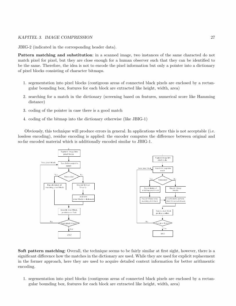
Pattern matching and substitution: in a scanned image, two instances of the same characted do notmatch pixel for pixel, but they are close enough for a human observer such that they can be identified tobe the same. Therefore, the idea is not to encode the pixel information but only a pointer into a dictionaryof pixel blocks consisting of character bitmaps.
1. segementation into pixel blocks (contigeous areas of connected black pixels are enclosed by a rectan-gular bounding box, features for each block are extracted like height, width, area)
2. searching for a match in the dictionary (screening based on features, numerical score like Hammingdistance)
3. coding of the pointer in case there is a good match
4. coding of the bitmap into the dictionary otherwise (like JBIG-1)
Obviously, this technique will produce errors in general. In applications where this is not acceptable (i.e.lossless encoding), residue encoding is applied: the encoder computes the difference between original andso-far encoded material which is additionally encoded similar to JBIG-1.
Soft pattern matching: Overall, the technique seems to be fairly similar at first sight, however, there is asignificant difference how the matches in the dictionary are used. While they are used for explicit replacementin the former approach, here they are used to acquire detailed context information for better arithmenticencoding.
1. segementation into pixel blocks (contigeous areas of connected black pixels are enclosed by a rectan-gular bounding box, features for each block are extracted like height, width, area)

KAPITEL 3. IMAGE COMPRESSION 28
2. searching for a match in the dictionary (screening based on features, numerical score like Hammingdistance)
3. coding of the pointer in case there is a good match
4. coding of the bitmap into the dictionary otherwise (like JBIG-1)
5. coding of the bitmap of the current block (the centers of the two matching blocks are aligned and thepixels are arithmetically encoded using the two contexts shown in the figure below).
As a result, a poor match does not result in an error as it occurs in the first approach but only in a lessefficient encoding due to incorrect context information.
Halftone data
There are also two ways how to encode halftone data. The first approach uses a classical arithmetic codingtechnique close to JBIG-1, however, the context used is larger (up to 16 pixels) and may include up to 4adaptive pixels as shown in the figure. This is important to capture regularities in the halftoning patternsbetter.

KAPITEL 3. IMAGE COMPRESSION 29
The second approach relies on descreening the halftone image (converting it back to grayscale) using animage tiling (where the grayscale value can be e.g. the sum of the set pixels in the block). The grayscaleimage is represented in Gray code (see below) and the bitplanes are arithmetically encoded similar to JBIG-1. The grayscale values are used as indices of fixed-size bitmap patterns in a halftone bitmap directory.Therefore the decoder applies simple lookup-table operations.
Apart from the loss already potentially introduces by some of the techniques, additional techniquesto reduce the amount of data in a lossy manner may be employed: quantization of pixel-block positioninformation, noise removal and smoothing, and explicit bit-flipping for entropy reduction.
3.1.4 Compression of Grayscale Images with JBIG
Like any other technique for compressing binary images, JBIG can be used to compress grayscale data. Thisis accomplished by successive coding of single bitplanes (which are binary images of course), e.g. we start withfusing the MSBs of all pixels into a bitplane, compress it, and carry on until we have compressed the bitplanecontaining all LSBs. All typical compression systems are able to take advantage of large aras of uniformcolour. Therefore, the bitplanes should preferably like this. However, the classical binary representationleads to the opposite effect. Consider large areas in the original image where the grayscale changes from127 to 128. In binary representation this corresponds to 01111111 and 10000000 which means that a changefrom 127 to 128 causes a bitchange in each bitplane which destroys large nearly uniform areas found inthe original image in the bitplanes. This problem can be overcome by employing the Gray Code. In Graycode representation, two neighbouring decimal number only differ in a single bit in their respective binaryrepresentation. This is exactly what we want.
Binary Code −→ Gray Code:
1. Starting with the MSB of the original binary representation, all 0 are kept until we hit a 1.
2. The 1 is kept, all following bits are inverted until we hit a 0.
3. The 0 is inverted, all following bits are kept, until we hit a 1.
4. Goto Step 2.
Gray Code −→ Binary Code:
1. Starting with the MSB of the Gra code representation, all 0 are kept until we hit a 1.
2. The 1 is kept, all following bits are inverted until we hit a 1.
3. The 1 is inverted, all following bits are kept, until we hit a 1.
4. Goto Step 2.

KAPITEL 3. IMAGE COMPRESSION 30
3.1.5 Lossless JPEG
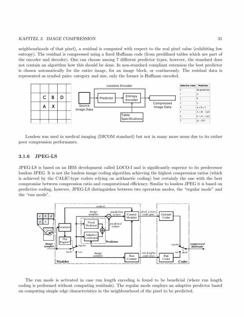
Up to 6bpp we get decent results with successive JBIG encoding, for higher bit-depth other techniquesshould be used which are better able to exploit the inter-bitplane dependencies. The simplest choice forthis application is the standard for lossless image compression developed by the Joint Photographic ExpertsGroup (JPEG): lossless JPEG is a classical DPCM coder (and has nothing to do with the JPEG format weall know from digital cameras !). Based on a prediction for the actual pixel that should be encoded (involving
KAPITEL 3. IMAGE COMPRESSION 31
neighbourhoods of that pixel), a residual is computed with respect to the real pixel value (exhibiting lowentropy). The residual is compressed using a fixed Huffman code (from predifined tables which are part ofthe encoder and decoder). One can choose among 7 different predictor types, however, the standard doesnot contain an algorithm how this should be done. In non-standard compliant extension the best predictoris chosen automatically for the entire image, for an image block, or contineously. The residual data isrepresented as symbol pairs: category and size, only the former is Huffman encoded.
Lossless was used in medical imaging (DICOM standard) but not in many more areas due to its ratherpoor compression performance.
3.1.6 JPEG-LS
JPEG-LS is based on an IBM development called LOCO-I and is significantly superior to its predecessorlossless JPEG. It is not the lossless image coding algorithm achieving the highest compression ratios (whichis achieved by the CALIC-type coders relying on arithmetic coding) but certainly the one with the bestcompromise between compression ratio and computational efficiency. Similar to lossless JPEG it is based onpredictive coding, however, JPEG-LS distinguishes between two operation modes, the “regular mode” andthe “run mode”.
The run mode is activated in case run length encoding is found to be beneficial (where run lengthcoding is performed without computing residuals). The regular mode employs an adaptive predictor basedon computing simple edge characteristics in the neighbourhood of the pixel to be predicted.

KAPITEL 3. IMAGE COMPRESSION 32
In case a vertical edge is detected left to X, this predictor tends to predict a, in case a horizontal edgeis found above X, the predictor tends to predict b, in case no edge is detected a plane-focused prediction isdone. To see this, let us assume a ≤ b: either (1) c ≥ b means a vertical edge and min(a, b) = a is predicted,in case (2) c ≤ a means a horizontal edge and max(a, b) = b is predicted.
When considering a plane spanned among the points a, b, c,X this can be seen easily. Moreover it getsclear that averaging a, b, c is not a very good idea in case there is no edge. The predictor is also interpreteddifferently, as being the median of three fixed predictors a, b, a + b − c – and is therefore also termed as“median edge detector (MED)”.
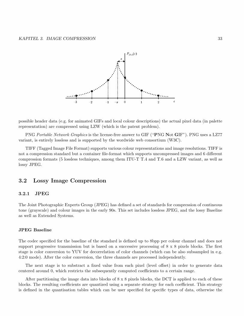
After the prediction has been computed, the distribution of residual values is estimated based on contextinformation. Residual values in general are known to be of two-sided geometrical distribution, the actualshape of the distribution is determined based on context information. In order to derive contexts, thequantities d− a, a− c, and c− b are computed and quantized to result in 365 different contexts. Accordingto the estimated distribution shape parameter, the values are encoded using Rice-Golumb codes (which areknown to be optimal for geometric distributions.
3.1.7 GIF, PNG, TIFF
The GIF (Graphics Interchange Format) standard is a proprietory CompuServe format (which was not allall known when it became that popular as it is topday). For historical reasons (nobody believed in 1987 thatit could ever be necessary to represent more than 256 colours on a computer screen) the number of coloursthat can be represented is restricted to 256 (out of 16 million for true colour images). This means that formore colours quantisation is applied (which means that compression is lossy). Apart from a huge number of
KAPITEL 3. IMAGE COMPRESSION 33
possible header data (e.g. for animated GIFs and local colour descriptions) the actual pixel data (in paletterepresentation) are compressed using LZW (which is the patent problem).
PNG Portable Network Graphics is the license-free answer to GIF (“PNG Not GIF”). PNG uses a LZ77variant, is entirely lossless and is supported by the wordwide web consortium (W3C).
TIFF (Tagged Image File Format) supports various colour representations and image resolutions. TIFF isnot a compression standard but a container file-format which supports uncompressed images and 6 differentcompression formats (5 lossless techniques, among them ITU-T T.4 and T.6 and a LZW variant, as well aslossy JPEG.
3.2 Lossy Image Compression
3.2.1 JPEG
The Joint Photographic Experts Group (JPEG) has defined a set of standards for compression of contineoustone (grayscale) and colour images in the early 90s. This set includes lossless JPEG, and the lossy Baselineas well as Extended Systems.
JPEG Baseline
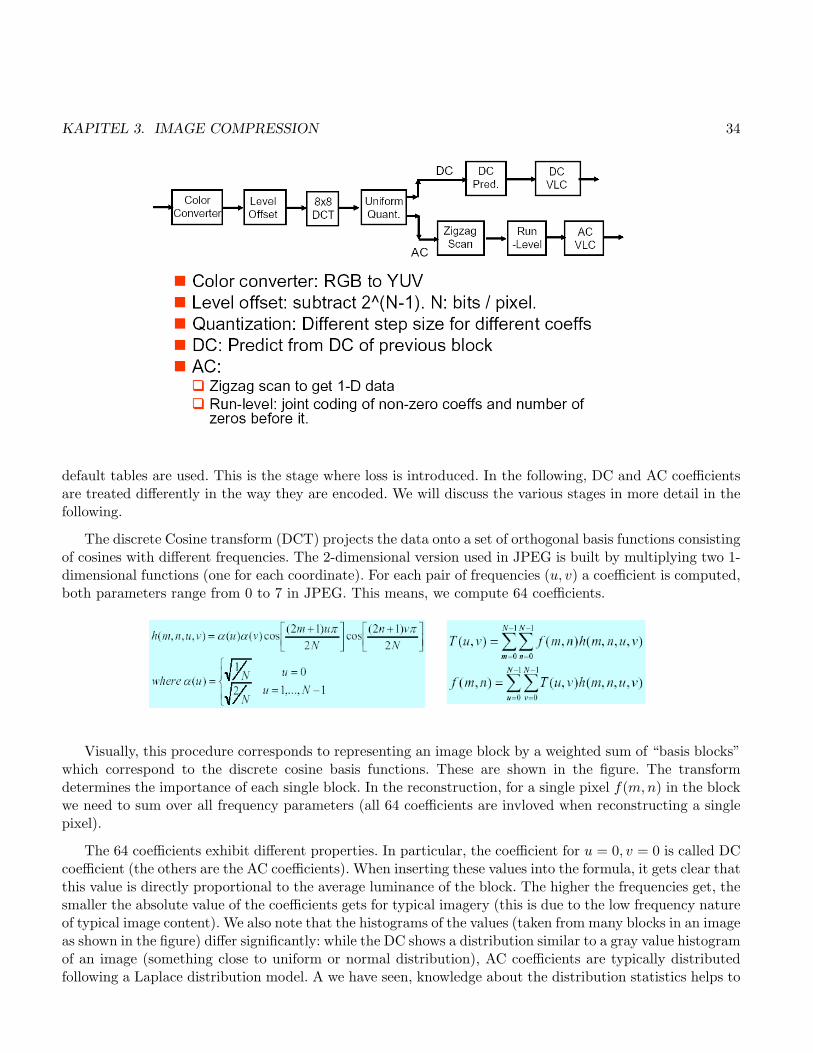
The codec specified for the baseline of the standard is defined up to 8bpp per colour channel and does notsupport progressive transmission but is based on a successive processing of 8 x 8 pixels blocks. The firststage is color conversion to YUV for decorrelation of color channels (which can be also subsampled in e.g.4:2:0 mode). After the color conversion, the three channels are processed independently.
The next stage is to substract a fixed value from each pixel (level offset) in order to generate datacentered around 0, which restricts the subsequently computed coefficients to a certain range.
After partitioning the image data into blocks of 8 x 8 pixels blocks, the DCT is applied to each of theseblocks. The resulting coefficients are quantized using a separate strategy for each coefficient. This strategyis defined in the quantisation tables which can be user specified for specific types of data, otherwise the
KAPITEL 3. IMAGE COMPRESSION 34
default tables are used. This is the stage where loss is introduced. In the following, DC and AC coefficientsare treated differently in the way they are encoded. We will discuss the various stages in more detail in thefollowing.
The discrete Cosine transform (DCT) projects the data onto a set of orthogonal basis functions consistingof cosines with different frequencies. The 2-dimensional version used in JPEG is built by multiplying two 1-dimensional functions (one for each coordinate). For each pair of frequencies (u, v) a coefficient is computed,both parameters range from 0 to 7 in JPEG. This means, we compute 64 coefficients.
Visually, this procedure corresponds to representing an image block by a weighted sum of “basis blocks”which correspond to the discrete cosine basis functions. These are shown in the figure. The transformdetermines the importance of each single block. In the reconstruction, for a single pixel f(m,n) in the blockwe need to sum over all frequency parameters (all 64 coefficients are invloved when reconstructing a singlepixel).
The 64 coefficients exhibit different properties. In particular, the coefficient for u = 0, v = 0 is called DCcoefficient (the others are the AC coefficients). When inserting these values into the formula, it gets clear thatthis value is directly proportional to the average luminance of the block. The higher the frequencies get, thesmaller the absolute value of the coefficients gets for typical imagery (this is due to the low frequency natureof typical image content). We also note that the histograms of the values (taken from many blocks in an imageas shown in the figure) differ significantly: while the DC shows a distribution similar to a gray value histogramof an image (something close to uniform or normal distribution), AC coefficients are typically distributedfollowing a Laplace distribution model. A we have seen, knowledge about the distribution statistics helps to

KAPITEL 3. IMAGE COMPRESSION 35
gain in compression efficiency.
The next stage in the process is to apply quantization to the computed transform coefficients. The basicoperation is to divide the coefficient Yij by a value Qij and round the result to integer. It is important tonote that Qij is potentially different for each coefficient and is defined in the so-called quantisation tables.
Quantisation tables usually differ between luminance and color components and are provided in the formof default tables as shown in the figure. In case data with some specific properties are compressed, these tablescan also be specified differently and optimised for a specific taget application (e.g. for fingerprint images,iris images, satellite images etc.). In this case, the tables are communicated to the decoder in the header ofthe compressed file. Note that the default tables have been optimised based on large scale experimentationinvolving thousands of subjects.
The fundamental idea in the quantisation table design is to quantise coefficients which correspond to“irrelevant” visual information more severly. This essentially means that the higher the frequency gets, themore severe quantisation is being applied. In order to “survive” quantisation, a high frequency coefficientneeds to exhibit a significant size (i.e. the corresponding visual information needs to be really important).
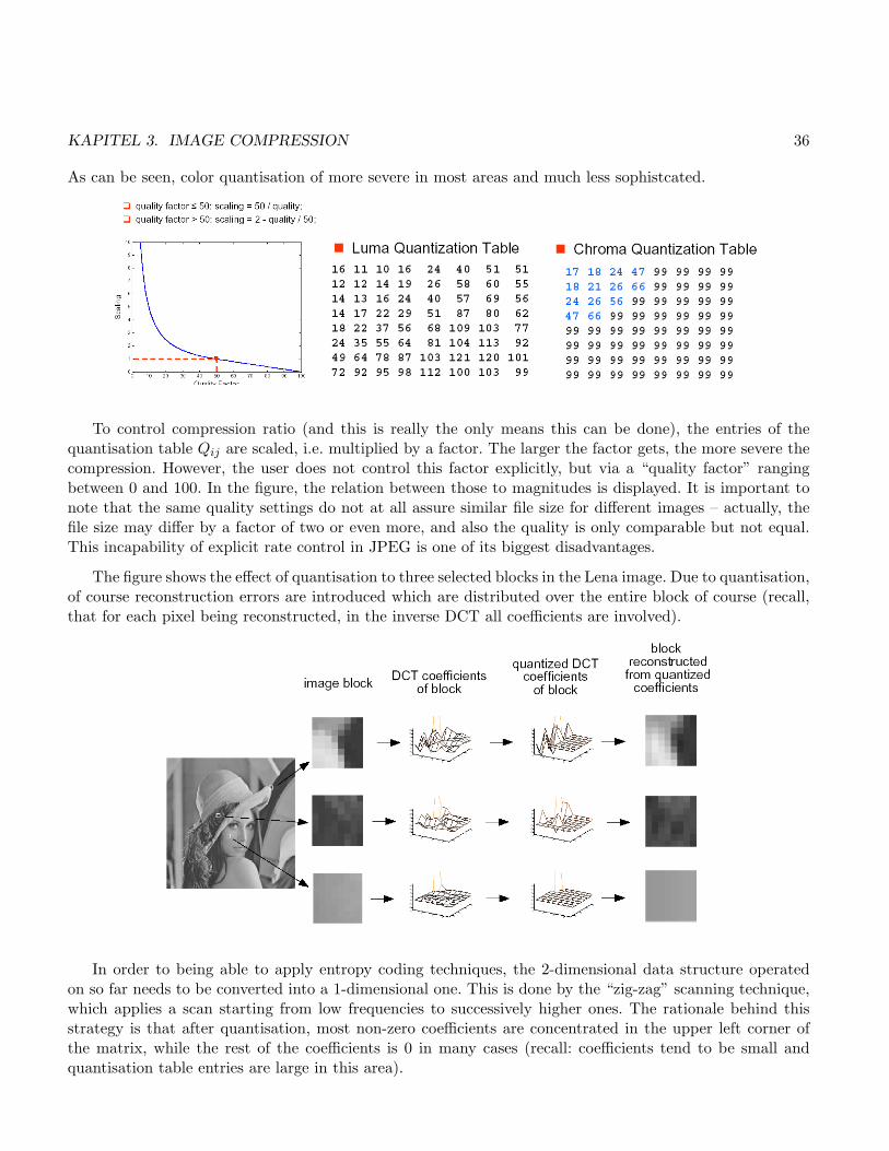
KAPITEL 3. IMAGE COMPRESSION 36
As can be seen, color quantisation of more severe in most areas and much less sophistcated.
To control compression ratio (and this is really the only means this can be done), the entries of thequantisation table Qij are scaled, i.e. multiplied by a factor. The larger the factor gets, the more severe thecompression. However, the user does not control this factor explicitly, but via a “quality factor” rangingbetween 0 and 100. In the figure, the relation between those to magnitudes is displayed. It is important tonote that the same quality settings do not at all assure similar file size for different images – actually, thefile size may differ by a factor of two or even more, and also the quality is only comparable but not equal.This incapability of explicit rate control in JPEG is one of its biggest disadvantages.
The figure shows the effect of quantisation to three selected blocks in the Lena image. Due to quantisation,of course reconstruction errors are introduced which are distributed over the entire block of course (recall,that for each pixel being reconstructed, in the inverse DCT all coefficients are involved).
In order to being able to apply entropy coding techniques, the 2-dimensional data structure operatedon so far needs to be converted into a 1-dimensional one. This is done by the “zig-zag” scanning technique,which applies a scan starting from low frequencies to successively higher ones. The rationale behind thisstrategy is that after quantisation, most non-zero coefficients are concentrated in the upper left corner ofthe matrix, while the rest of the coefficients is 0 in many cases (recall: coefficients tend to be small andquantisation table entries are large in this area).

KAPITEL 3. IMAGE COMPRESSION 37
When considering the example result of the scanning process, we note that for increasing frequency, theruns of 0s get longer and 0 runs in general appear more often. This is also the reason for conducting the scanin this manner. The scanned data is then converted into a (run,level)-pair representation: run determines thenumber of preceeding zero coefficients and level is the actual magnitude of the coefficient. The DC coefficientis not included in the scan as it is coded separately. The data corresponding to a block is terminated by theEOB symbol, which also states that the non-coded coefficients before it are all 0.
However, coefficient magnitude (the range information) is not encoded directly in JPEG. Instead, a twolayered way of representing the data has turned out to be more beneficial: the first layer (the category)determines the approximate size of the range, subsequently the actual value in this category is encoded. Thefigure shows the different categories for DC and AC coefficients together with their corresponding ranges.Note that the number of values in the different categories differs, i.e. increases for larger range values.
Differential encoding is applied to DC coefficients (note that this is the only part of the standard whereinter-block correlations are exploited), and the prediction error is encoded using a VLC (Huffman codewords)for the category of the prediction error, index coding (i.e. the position in the category) is used to representthe value inside the category. The number of the category determines the number of bits maximally requiredto code the index.
The AC coefficient (run,level)-pairs are encoded differently. The 8 bit information NNNNSSSS (whereNNNN is the run information and SSSS is the category information) is encoded in a Huffman codeword(fixed code), while the information about the actual value in the category is encoded like in the DC case inan index coding scheme.
In the figure the entire processing chain of encoding and decoding a single block is visualised. For de-

KAPITEL 3. IMAGE COMPRESSION 38
quantisation, the decoded coefficient values are simply multiplied by the scale value used during compression(this value needs to be communicated in the header, which is identical for each block in the case of JPEGbut not in MPEG). Note that after inverse DCT, the error is dispersed among all pixels of the block.
The example shows typical JPEG quantisation errors: for high compression ratios, the block boundariesare clearly visible. For many blocks, only the DC coefficient is retained causing a uniform gray block in thereconstruction. Adjacent blocks with different gry value exhibit very disturbing boundaries.
A JPEG file is highly structured. A frame is a single picture which is preceeded by the main headerand terminated by another marker sequence. A frame is composed of several scans, which are preceeded bycorresponding table and header information (a scan usually corresponds to a spectral / color band). Thenext bitstream entity is a collection of segments (which is again preceeded by table and header information).A segment is composed of a couple of adjacent 8 x 8 pixel blocks.

KAPITEL 3. IMAGE COMPRESSION 39
JPEG had tremendous impact and is still the most widely used format for lossy grayscale and color imagecompression. The algorithm is very fast and due to the block-based processing it requires a small amountof memory only. On the other hand, the quality at low bitrates (i.e. high compression ratios) is limited, andthe lack of exlicit rate-control is very inconvenient for transmission-based applications for example.
JPEG Extended System
The extended system adds support for data up to 12 bpp, optional arithmetic encoding of coefficients, andmost importantly, progressive organisation of data. While in case of baseline JPEG, after interruption of afile transfer, an image is decoded only partially (depending on the number of blocks transmitted), progressiveJPEG variants allow a reconstruction of the entire image based on only partially transmitted information.However, of course the quality of the data is reduced as compared to the original version. In progressive
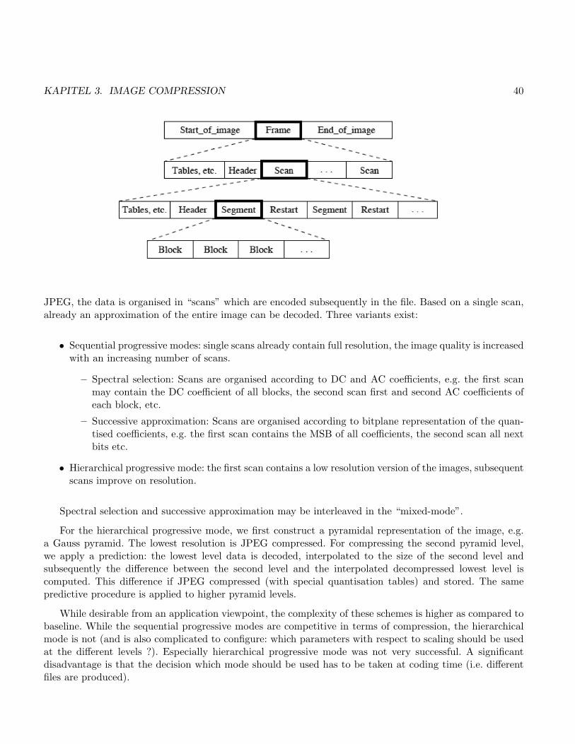
KAPITEL 3. IMAGE COMPRESSION 40
JPEG, the data is organised in “scans” which are encoded subsequently in the file. Based on a single scan,already an approximation of the entire image can be decoded. Three variants exist:
• Sequential progressive modes: single scans already contain full resolution, the image quality is increasedwith an increasing number of scans.
– Spectral selection: Scans are organised according to DC and AC coefficients, e.g. the first scanmay contain the DC coefficient of all blocks, the second scan first and second AC coefficients ofeach block, etc.
– Successive approximation: Scans are organised according to bitplane representation of the quan-tised coefficients, e.g. the first scan contains the MSB of all coefficients, the second scan all nextbits etc.
• Hierarchical progressive mode: the first scan contains a low resolution version of the images, subsequentscans improve on resolution.
Spectral selection and successive approximation may be interleaved in the “mixed-mode”.
For the hierarchical progressive mode, we first construct a pyramidal representation of the image, e.g.a Gauss pyramid. The lowest resolution is JPEG compressed. For compressing the second pyramid level,we apply a prediction: the lowest level data is decoded, interpolated to the size of the second level andsubsequently the difference between the second level and the interpolated decompressed lowest level iscomputed. This difference if JPEG compressed (with special quantisation tables) and stored. The samepredictive procedure is applied to higher pyramid levels.
While desirable from an application viewpoint, the complexity of these schemes is higher as compared tobaseline. While the sequential progressive modes are competitive in terms of compression, the hierarchicalmode is not (and is also complicated to configure: which parameters with respect to scaling should be usedat the different levels ?). Especially hierarchical progressive mode was not very successful. A significantdisadvantage is that the decision which mode should be used has to be taken at coding time (i.e. differentfiles are produced).

KAPITEL 3. IMAGE COMPRESSION 41
3.2.2 Wavelet-based Image Compression
The Wavelet Transform
When employing the Fourier Transform, we are not able to manipulate frequency locally. In case we modify atransform coefficient, this change is reflected in the entire signal (recall that for reconstructing a single pixel,all coefficients / basis functions are involved). For this reason the windowed Fourier Transform (of ShortTime Fourier Transform STFT) has been introduced. To obtain corresponding basis functions, a Fourierbasis function is modulated with a window function which is zero outside of some interval. With this trick,the FT can be made localized (to make it simple this can be seen as cutting a signal into pieces and applying

KAPITEL 3. IMAGE COMPRESSION 42
the FT onto these pieces independently). Since the window has to be defined somehow, we are facing intrinsiclimitations: small windows do not capture low frequencies well, and vice versa, large windows do not captureshortlived high frequency phenonema well. The wavelet (i.e. little wave, cf. ondelette in French) transformoffers a more general solution to this problem:
Wa,b(f) = |a|−1/2
∫ ∞
−∞f(t)ψ
(t− b
a
)dt (3.1)
ψa,b(s) = |a|−1/2ψ
(s− b
a
)(3.2)
The functions in equation (3.2) are termed wavelets, ψ(s) is called “mother wavelet” as it is the proto-typical function. Examples of some mother wavelets are:
ψ(s) = (1− s2)es2
2 Mexican Hat (3.3)
ψ(s) =sin(2πs)− sin(πs)
πsShannon Wavelet (3.4)
ψ(s) =
1 0 ≤ s ≤ 1/2−1 1/2 ≤ s ≤ 10 otherwise
Haar Wavelet (3.5)
The wavelet transform depends on two parameters a and b. In case a changes, the wavelets in equation(3.2) cover different “frequency bands” by changing the scale of the function: larger a lead to broad functionsbetter suited to capture low frequency parts of the signal, while small a lead to slim functions suited betterto represent high frequency parts of the signal. In case b changes, the localisation-center of the function(which is in s = b) is shifted. All wavelet functions are shifted and scaled versions of the mother wavelet.
Multiresolution Analysis (MRA) is the concept that is used to derive a fast algorithm and (bi)orthogonalwavelet basis functions with compact support. One of the fundamental problems in wavelet analysis isthat functions unifying these desired properties do not have a closed expression in the time domain. Thebackground of this approach is to represent a signal by differently scaled approximations of the signal
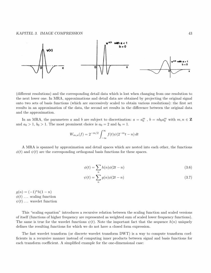
KAPITEL 3. IMAGE COMPRESSION 43
(different resolutions) and the corresponding detail data which is lost when changing from one resolution tothe next lower one. In MRA, approximations and detail data are obtained by projecting the original signalonto two sets of basis functions (which are successively scaled to obtain various resolutions): the first setresults in an approximation of the data, the second set results in the difference between the original dataand the approximation.
In an MRA, the parameters a and b are subject to discretisation: a = am0 , b = nb0a
m0 with m,n ∈ Z
and a0 > 1, b0 > 1. The most prominent choice is a0 = 2 and b0 = 1.
Wm,n(f) = 2−m/2
∫ ∞
−∞f(t)ψ(2−mt− n) dt
A MRA is spanned by approximation and detail spaces which are nested into each other, the functionsφ(t) and ψ(t) are the corresponding orthogonal basis functions for these spaces.
φ(t) =∑
n
h(n)φ(2t− n) (3.6)
ψ(t) =∑
n
g(n)φ(2t− n) (3.7)
g(n) = (−1)nh(1− n)φ(t) . . . scaling functionψ(t) . . . wavelet function
This “scaling equation” introduces a recursive relation between the scaling function and scaled versionsof itself (functions of higher frequency are represented as weighted sum of scaled lower frequency functions).The same is true for the wavelet functions ψ(t). Note the important fact that the sequence h(n) uniquelydefines the resulting functions for which we do not have a closed form expression.
The fast wavelet transform (or discrete wavelet transform DWT) is a way to compute transform coef-ficients in a recursive manner instead of computing inner products between signal and basis functions foreach transform coefficient. A simplified example for the one-dimensional case:

KAPITEL 3. IMAGE COMPRESSION 44
input = (a, b, c, d, e, f, . . .) h(n) = (1, 2, 3, 4)WT1 = a+ 2b+ 3c+ 4dWT2 = b+ 2c+ 3d+ 4e
detail signal
h
h
g
g
This procedure can also be interpreted as cascading low and high pass filters: the filters correspondingto the approximation spaces (scaling function) act as low pass filters, the detail space filters act as high passfilters (wavelet function). Variants how to deal with the signals edge (from stupid to more sensible):
• Zero-Padding
• Periodisation
• Signal extension (copying)
• Mirroring
For decomposing images we require the transformation of two-dimensional functions. First, we transformthe images lines, subsequently we apply the trnaformation to the already transformed columns of the image.By analgy to the one-dimensional case, we apply downsampling by 2 in both directions. The following figuresillustrate this process.
We note that in the detail subbands, we notice edge information related to image content. In particular,the edge information is different with respect to the edge-orientation information: in two subbands, we seemainly vertical and horizontal edge information (here, the high pass part was applied in either horizontal orvertical direction only, i.e. to lines and columns), while one subband corresponds to diagonal edge information(this is where the high pass filter has been applied to both lines and columns).
In case of the Fourier transform a single coefficient represents the frequency content of the entire imagewith respect to the frequencies u and v. In case of the wavelet transform a single coefficient represents theenergy content in a frequency band at a specific location / position in the image. By gaining localisation inthe spatial / time domain, we sacrifice localisation in the frequency band. Therefore, it depends on the typeof application, which is the more suited transform (global frequency descriptions vs. localised ones).

KAPITEL 3. IMAGE COMPRESSION 45
row filtering / downsampling
colu
mn filte
ring / d
ow
nsam
plin
g
original
image
h
g
h
g
h
g
detail
detaildetail
LL
horizontal low-pass
horizontal high-pass
vertical low-pass
vertical high-pass
This is a very general phenonemon: we cannot have both perfect frequency and time / space localisationin time-frequency analysis; while the FT is one extremal point of the spectrum, on the other end we haveimpulses (or Dirac functions), wavelets range somewhere in-between.
In the example shown, we exploit the advantage of the availability of localized frequency informationin denoising. The displayed music signal contains “pop noise” which can originate from disc scratches ormicrophone artifacts. The FT domain does not any specific signs of that (rather high frequency) noise, so

KAPITEL 3. IMAGE COMPRESSION 46
second filtering step third filtering step
Fourier Wavelet
high frequency low frequency
we apply a classical low-pass filtering.
When considering the result, it get clear that the pop noise has been removed successfully. On the otherhand, we of course also “succeeded” in removing the high frequency parts of the music signal resulting insignificantly reduced quality.
When analysing the signal with a WT (note that in the example, the subsampling stage has beenavoided), we note distinct spikes at three different locations spread accross several subbands. This meansthat while being of high frequency in general, the noise is spread across a couple of frequency bands whichmakes it specifically difficult to remove with a global low pass filtering. In the wavelet domain, the classical

KAPITEL 3. IMAGE COMPRESSION 47
denoising approach is to threshold the detail subband coefficients (the assumption is that coefficients affectedby noise have a high energy).
When applying this technique to our data we realize that in the reconstructed data, high frequencycontent has been preserved on the one hand, on the other hand the spikes of the pop noise have beenremoved successfully.
The wavelet packet transform generalises the DWT by also conducting a recursive decomposition proce-dure to the high frequency subband. The result is a balanced tree which implies also a balanced frequencyresolution among the subbands generated. When considering the entire tree of subbands, it is no longer clearwhich subbands should be used to represent a signal (which are best suited in terms of compression). Inorder to adaptively determine the most suited set of subbands, the “best basis algorithm” can be applied:in the fully decomposed tree, a cost function is computed for each subband. Subsequently, starting from thebottom of the tree, we compare the costs of a parent leave with the sum of the costs of the children leaves(note that the cost functions should be additive to allow fast computation). If the cost of the parent is higher,this decomposition stage is profitable and we assign the costs of the children to the parent node indicating“decompose”. This scheme is applied recursively until we end up at the top of the tree. JPEG2000 Part 2

KAPITEL 3. IMAGE COMPRESSION 48
allows to apply this scheme and the FBI fingerprint standard uses a fixed WP decomposition structure toaccount for the high frequency nature of fingerprint images.
First Generation Techniques
Techniques of this type have been developed soon after the DWT has been introduced in the mid 90s. Theyfollow the classical scheme of transform coding (transform – quantisation – entropy coding) and simplyreplace the block-based DCT by the WT. As it can be expected, the gain as compared to JPEG for examplewas not significant in most cases. However, Analog Devices developed a chip for hardware-based waveletimage compression (ADV 401) using a very simple technique and the abovementioned FBI fingerprintcompression standard also uses an approach like this.
Second Generation Techniques: Zerotrees
These schemes try to exploit an almost obvious property of the wavelet transform domain: the similarity ofdetail subbands across scales. First attempts try to accomplish this in a direct manner by predicting higherfrequency subbands by interpolated versions of their lower frequency counterparts of the same orientation.Also, significant effort has been invested into exploiting these self-similarities by means of fractal compressionin the wavelet domain (however, after is has been found that spatial domain fractal coding can be interpretedas a sort of simple wavelet based coding with specific filters these attempts have no longer been made).
The key concept for exploiting inter-subband correlations is the idea of zero-trees. The correspondingzerotree hypothesis is stated as follows: “In case a WT coefficient is found to be insignificant with respect toa threshold T at a lower resolution, it is likely that its decendants in higher resolutions are also insignificantwith respect to T.” Due to the spatial relation of the coefficients tree stuctures across subbands can beestablished which can be encoded very efficiently. In case we observe an insignificant (e.g. zero after quan-tisation) coefficient at some resolution, we scan its corresponding children coefficients at higher resolutionsfor being insignificant as well. In case this property holds, we encode the coefficient at the lower resolutionas zero-tree root ZTR. As a consequence, all its decendants do not have to be encoded. For example, incase a zerotree spans across three resolutions, we encode 21 coefficients by the single ZTR symbol.
The procedure as established by “embedded zerotree wavelet” (EZW) coding is motivated by two reasons:First, contrasting to DCT based schemes edge-like structures are represented by only a few coefficients (as

KAPITEL 3. IMAGE COMPRESSION 49
opposed to DCT where this information is spread across many high frequency coefficients) of the wavelettransform – however, we need to efficiently encode the position information of these coefficients. Second, thereis great interest in establishing embedded / scalable dataformats which are intrinsically suited for progressivetransmission (embedded: having all lower bit rate codes of the same image embedded at the begin of the bitstream, bits are generated in the order of importance and the encoder can terminate encoding at any pointallowing a target bitrate to be met exactly).
The procedure starts by defining an initial threshold T = bMaxCoeff/2c. The idea is to generate a“significance map” which encodes the positions of coefficients which are found to be significant with respectto a given threshold. Note that this corresponds to an analysis for which coefficients bits are set in the MSBbitplane.
After a complete scan over the transformed image has been done, the threshold is divided by two andagain, significance is determined against this new threshold. This corresponds to the analysis of the nextbitplane. This procedure is repeated until all bitplanes are processed.
For each bitplane, the coefficient information is encoded in two passes: the significant pass (dominantpass) and the refinement pass (subordinate pass). At initialisation, all coefficients are insignificant.
In the significance pass, four syntax symbols are used to encode information about the coefficients thathave not been found significant so far in previous passes. For significant coefficients, significant positive (SP)or significant negative (SN) is encoded. For insignificant coefficients, either ZTR (in case all decendants areinsignificant) or isolated zero (IZ) is encoded. At the highest frequency subband, ZTR and IZ are reduced intoa single symbol. The coefficients for which SP or SN is coded are added to the list of significant coefficients.
In the refinement pass, an additional bit of the binary representation of coefficients already found to be

KAPITEL 3. IMAGE COMPRESSION 50
significant is encoded. The scan order follows the scheme depicted in the figure concerning subbands, insidesubbands coefficients are simply scanned line by line.
The symbols output by the embedded coding procedure are finally arithmetically encoded. Due to thefact that we have four different symbols, a non-binary variant has to be employed. For the significance pass4 contexts are used depending on the significance of the parent and immediately neighbouring coefficients.Refinement data uses a single context.
In the reconstruction process it should be noted that bitplane encoding corresponds to uniform quanti-sation with deadzone.
For SP, we set 1.5T, for SN we set -1.5T, and 0 for ZTR and IZ. Based on the refinement bits, coefficientsare successively reconstructed with more accuracy. Note that this perfectly allows embedded decoding ofthe data where decoding may stop at any coefficient position.
The processing of the lists has turned out not to result in the best possible compression and computationperformance. As a consequence a technique termed “set partitioning in hierarchical trees (SPIHT)” has beendeveloped, which replaces the lists by sets of coefficients and achieves even better compression performance.
Mainly due to patent-related issues but also due to the fact that the exploitation of inter-subbandcorrelations in expensive in terms of computation and memory requirements, zerotree-based schemes havenot been considered in the context of JPEG2000 standardisation.

KAPITEL 3. IMAGE COMPRESSION 51
Third Generation Techniques: JPEG2000
JPEG follows an “old” coding paradigm in the sense that for serving a specific application, a specificencoding option has to be used to produce an application specific file (lossless vs. lossy, progressive or not,hierarchical vs. sequential progressive). This means, that this decision has to be taken at encoding time.If a different application should be served based on an older bitsream, usually transcoding into a differentformat is required.
Therefore, JPEG2000 has been designed following a “new” coding paradigm where a generic bitstream isproduced, out of which different bitstreams can be extracted allowing for adaptation to different applicationneeds. No coding decision has to be taken at encoding time (apart from that if quantisation is applied, thereconstructed data is always lossy of course), the decisions which parts of the data are used to reconstructimage material is done at decoding time. This makes the format highly flexible but implies on the otherhand, that the informations required for flexible decoding have to be present in the bitstream.
JPEG2000 is not based on zerotree encoding since
• there are many patent issues with zerotree codecs,
• the irregular coding structure traversing many subbands imply high memory consumption and expen-sive hardware design, and
• zerotree coding offers no resolution scalability.
All functionalities supported by the various flavours of JPEG are supported by a single bitstream (los-sless + lossy, different types of progressiveness), better quality at low bitrates and explicit rate-control arefeatured. JPEG2000 is a typical transform coding scheme which is based on the DWT and follows thefollowing stages.
• For large images, optional tiling is applied, i.e. cutting the image into smaller pieces where each tileis subsequently compressed independently. For small images, there is only one tile consisting of theimage itself.
• DC-level shift: the image data is transformed to result in approximately zero mean, i.e. for 8 bpp data,128 is subtracted from each pixel.

KAPITEL 3. IMAGE COMPRESSION 52
• For classical (RGB) color images, a “multi component transform” is applied, decorrelating the colorbands.
• The DWT is applied to each tile independantly.
• Uniform quantisation with a deadzone quantiser is optionally applied (this leads to lossy compression),for a lossless stream this is skipped.
• After Quantisation, optional region of interest coding is applied.
• Tier-1 coding applies progressive arithmetic coding of coefficient binary representations within code-blocks.
• Tier-2 coding aggregates the final bitstream from all codeblock bitstreams in a rate-distortion optimalway
The color transform used in JPEG2000 comes in two flavours: one for lossless coding, the other onefor lossy coding. The lossy version is optimal in terms of decorrelation but leads to rounding errors, whilethe lossless one is an integer-based approximation of the lossy one and can be inversed without numericalerror. In case that it is clear the quantisation is applied when producing the final bitstream (i.e. target is a

KAPITEL 3. IMAGE COMPRESSION 53
minimal size of the bitstream but less generality), the irreversible mode should be used. In all other cases,the reversible scheme is preferable (which is also faster).
Image tiling is required only for very large images. When applied to small images, blocking artifactssimilar to those introduced in JPEG appear. This can be limited by using overlapped tiling. Still, tilingshould be restriced to VERY large image data !
Similar to the multi-component transform, also the DWT comes in two flavours in order to support lossyand lossless compression in an optimal manner. The lossless variant using 5/3 integer filters is based oninteger operations only and is therefore also faster as compared to the 9/7 floating precision filters for lossycoding, which are optimised for energy compactation.
After the DWT, the transform domain is partitioned into smaller squared units, so-called “codeblocks”(default size is 642 coefficients, a codeblock cannot be smaller than a subband, so codeblock size and de-composition depth need to be jointly adjusted). In the following, Tier-1 coding is applied to each of thesecodeblocks independently by first identifying suitable contexts the information of which is fed into an arith-metic coder.
For each codeblock, the result is an independent bitstream which is subsequently processed in Tier-2coding. Note the difference to zerotree-based schemes: in JPEG2000 we operate on coding units which areeven smaller as single subbands whereas in zerotree-based coding subband borders have been traversed.

KAPITEL 3. IMAGE COMPRESSION 54
Tier-1 encoding itself relies on coding the binary representation of the codeblocks’ coefficients based ontheir significance. Each coefficient contributes to several binary bitplanes. The first time (i.e. in the mostsignificant bitplane a “1” is set) a coefficient contributes to the binary representation, the sign is coded inaddition to the coefficients’ binary information.
The encoding starts with the first bitplane (beginning with the most significant bits) where the binaryrepresentation of a coefficient contributes a “1”. The number of empty bitplanes (“leading zero bitplanes”)is signalled in the bitstream.
Each bitplane of a codeblock is scanned in a predifined order: starting from top left, the first four bitsof the first colun are scanned, then the first four bits of the second column, until the entire width of thecodeblock is covered. Then the second four bits of the first column are scanned and so on. At the lower endof the codeblock the remaining scans per column may involve four or less bits. Each coefficient in a bitplaneis coded in one of three coding passes which are intended to estimate symbol probabilities of one out ofthree different classes of bits (the data in a codeblock associated with one of these passes is called chunk):
• Significance Propagation (skipped for the first bitplane)
• Magnitude Refinement (skipped for the first bitplane)
• Cleanup (Normalisation)
A coefficient is said to be significant at some bitplane if there is at least one non-null bit encoded inprevious bitplanes. If the most significant bitplane is being processed, all samples are predicted to remaininsignificant. This is the reason for skipping Significance Propagation and Magnitude Refinement for thefirst bitplane.
During the Significance Propagation pass, a bit is coded if its location is not significant so far, but atleast one of its eight-connected neighbours is significant (significance is predicted). For the encoding ninedifferent contexts are used (depending on which / how many neighbours are significant and in which subband/ at which decomposition level the codeblock is). If a coefficient is significant it is given a value of 1 forcreation of the context (and the sign is addiitonally encoded), otherwise 0. Significance Propagation onlyincludes only bits of coefficients that were insignificant and have a non-zero context, all other coefficientsare skipped. The context is passed to the arithmetic coder and the coding is performed.
The second pass is the Magnitude Refinement pass, during which all bits that became significant in aprevious bitplane are coded. In this pass, the bits from coefficients that are already significant (except thosethat have just become significant in the immediately preceeding significance propagation pass) are beingcoded. The context used is determined by the significance state of the neighbours and if this is the firstrefinement bit or not.

KAPITEL 3. IMAGE COMPRESSION 55
The final pass (Cleanup or Normalisation Pass) encodes all remaining bits that have not been coveredby the two previous coding passes (i.e. coefficients that are insignificant and had the context value 0 duringthe propagation pass). Beside the neighbour context, also run-length context can be used in case all fourlocations in the column of the scan are insignificant and each has only insignificant neighbours.
Overall, four different coding primitives are used, each of them associated with appropriate contexts,overall only 18:
• Zero Coding (ZC): used in the significance propagation and cleaup passes for the p-th bit if thecoefficient is not yet significant (0 if it is still insignificant at the current bitplane, 1 if becomessignificant).
• Sign Coding (SC): in the significance propagation and cleaup passes, used when a coefficient firstbecomes significant.
• Magnitude Refinement (MR): in the refinement pass to refine one more bit of a significant coefficient.
• Run-length Coding (RLC): in cleanup pass, used to code the significance of multiple consecutiveinsignificant coefficients.
While the output of cleanup passes is always arithmetically encoded, there is an option to restict arithme-tic coding for the other two passes to the four most significant bitplanes, while the remaining data is writtenin raw mode: arithmetic-coding bypass or lazy mode. This is used to trade of computational complexity forcoding efficiency.
In the figure we have a visualization of how the (chunks of the) three coding passes are distributedamong codeblocks in an entire wavelet decomposition tree. While in the lower frequency subbands, onlya single codeblock is contained in a subband, the number of codeblocks increases with the frequency. Theleading non-zero bitplane gets lower (resp. higher in number) as the frequency increases (this is due to thedecreasing magnitude of the coefficients as frequency increases). As can be seen, in this bitplane only chunkscorresponding to the Cleanup pass are present.
After the creation of the single bitstreams for each codeblock, Tier-1 encoding is finished. Subsequently,the final bitstream is assambled in Tier-2 coding.

KAPITEL 3. IMAGE COMPRESSION 56
For enabling Tier-2 coding, codeblocks are organised into three spatially consistent rectangles, so-called“precincts”: at each resolution level, a data structure (typically consisting of four codeblocks) from eachsubband is collected and fused forming the precinct. For each codeblock bitstream, the encoder storestemporal information with respect to possible truncation points and the resulting errors when actuallyusing these points. The main task of Tier-2 coding is to assemble the codeblock bitstreams into the finalbitstream using this stored temporal information in a rate-distortion optimal manner.
The smallest unit in the bitstream is a packet (body), which consists of code block chunks of eachcodeblock in a precinct. A collection of packets, one from each precinct of each resolution level, constitutesa (quality) layer. So, a packet can be interpreted as one quality increment for one resolution level at onespatial location (since precincts correspond to spatial locations). By analogy, a layer can be interpreted asone quality increment for the entire full resolution image. Each layer successively improves the image qualityso that the decoder is able to decode the codeblock contributions contained in each layer in sequence.

KAPITEL 3. IMAGE COMPRESSION 57
The information stored in the codeblock header is generated as follows. First, the information if datais contained in the packet is signalled. For each subband and each codeblock in the precinct inclusioninformation is encoded (if no new coding passes included skip codeblock): in case it is the first inclusion ofthe codeblock, the number of leading insignficant bitplanes is additionally coded, in any case the number ofnew coding passes (i.e. chunks) and corresponding length information is coded in a scheme called “tag-treecoding” (which is a quadtree based scheme). Bit stuffing is applied to prohibit appearance of certain markercodes.
Based on the temporal information stored with each codeblocks’ bitstream, it is determined how manychunks of each codeblock are fused into the first quality layer to obtain a certain target bitrste and distortion.Each subsequent layer is formed by optimally further truncating the codeblocks’ bitstreams. Rate controlcan be done in two manners: first, by adjusting quantiser step sizes, and second (which is computationallymore involved), by ommitting certain coding passes when building packets.
The final bitstream is organised as a succession of layers the number of which can be defined (thisdetermines the granularity of the progressiveness). Each component is encoded separately but the finalbitstream is interleaved on a layer basis.
There are four types of progressiveness possible for the final bitstream which are achieved by appropriateordering of the packets in the bitstream:
• quality progressiveness
• resolution progressiveness
• spatial location progressiveness
• component progressiveness
Once the bitstream has been assembled in a certain order, different types of progressiveness are obtainedby only reordering the bitstream and decoding the information in this diferent ordering (to enable this, thecorresponding information from packet headers need to be extracted and interpreted).
In the examples we see a schematical visualization of how the data is organized to obtain several qualityand resolution levels, respectively.
It should be noted that the high flexibility of the data format of JPEG2000 has to be paid with somerestrictions in terms of coding performance, which is due to the required packet header informations. In

KAPITEL 3. IMAGE COMPRESSION 58
order to limit this impact, a small number of quality layers has to be formed, which causes the number ofchunks included in each packet to be large thus minimizing the number of packets (and therefore packetheaders) which limits corresponding coding overhead. Nevertheless, the coding performance (especially inthe low bitrate area) when compared to JPEG is impressive.
Examples for Coding performance (at 0.125 bpp as compared to JPEG):
Region of interest coding is one of the remarkable properties of JPEG2000. This functionality is importantin applications where certain parts of the image are more important than others, which implies that itis desirable to encode these areas with higher quality. Also during transmission, these regions should be

KAPITEL 3. IMAGE COMPRESSION 59
transmitted first (or with higher priority). The standard does NOT define how a RoI information can begenerated (i.e. given an arbitrary image, how to automatically determine which areas should be the RoI),but does specify how these areas should be encoded based on a given RoI location information. Examplesfrom biometrics imagery: in surveillance video, face detection can be applied to identify faces and encodethose in a RoI in order to get better face recognition results. Similarily, eye detection can be applied to faceimages to identify iris data and encode these in a RoI in order to get better iris recognition results.
The RoI coding the Part 1 of the standard is based on the MAXSHIFT technique, while the more generalscaling-based technique and the sequence-based mode are covered in Part 2 of the standard. The general ideaof the general RoI idea is to scale (shift) coefficients such that the bits associated with the RoI are placed inhigher bitplanes than the bits associated with the background. As a result, during the encoding procedure,the most significant RoI bitplanes are placed in the bitstream before any background bitplanes. Dependingon the actual scaling values, the less important RoI bits may be encoded together with the non-RoI bits.
If the bitstream is truncated, or the encoding process is terminated before the whole image is fullyencoded, the RoI will be of higher fidelity than the rest of the image.
The general scaling-based RoI technique works as follows:
1. Compute DWT.
2. Based on the defined geometrical RoI information, the RoI mask is derived indicating the set ofcoefficients which is affected by RoI encoding.
3. Optional quantisation is applied.
4. The coefficients outside of the RoI are downscaled by a specified scaling value.
5. The resulting data is Tier-1 and Tier-2 encoded.
In the general scheme, the decoder requires the scaling value as used in the scaling and the geometricalRoI information which is included in the bitstream. In the specific MAXSHIFT technique of JPEG2000 ofPart 1, the scaling value is chosen in a way that the minimum coefficient belonging to the RoI is largerthan the maximum coefficient of the non-RoI areas. In decoding, the decoder simply scales up each non-RoIcoefficient.

KAPITEL 3. IMAGE COMPRESSION 60
An important advantage as compared to the general scaling mode is that the decoder does not needto have the geometrical RoI information due to the magnitude separation of the coefficients, which is goodwith respect to data amount (RoI information is not stored), encoder complexity (RoI information is notencoded), and decoder complexity (RoI is not decoded). Additionally, different bitrates (i.e. qualities) canbe defined for RoI and background (which cannot be done in the general scaling-mode). The disadvantage ascompared to the general scaling-based approach is a sightly increased datarate which is due to the separationof the data (context information can be expoited less efficiently).
Parts of the JPEG2000 standard suite:
1. Core coding system as being described.
2. Extensions: more flexible forms of decompositions (in terms of filters and subband structure), sequencemode in RoI coding, metadata sets and JPX as file format.
3. Motion JPEG 2000: defines a file format called MJ2 (or MJP2) for motion sequences of JPEG 2000images. Support for associated audio is also included.
4. Conformance: test procedures for conformance testing and bitstreams.
5. Reference software: JasPer (C) and JJ2000 (JAVA)
6. Compound image file format: JPM can be used to store multi-page documents with many objects perpage. Although it is a member of the JPEG 2000 family, it supports the use of many other coding orcompression technologies as well. For example, JBIG2 could be used for regions of text, and JPEGcould be used as an alternative to JPEG 2000 for photographic images.
7. abandoned
KAPITEL 3. IMAGE COMPRESSION 61
8. JPSEC (security aspects): Encryption, source authentication, data integrity, conditional access, ow-nership protection. The underlying techniques to protect the content include digital signatures, wa-termarking, encryption, scrambling, and key generation and management. These techniques will beenabled in JPSEC by means of a registration authority. More specifically, all techniques have to bepreviously registered in a central repository, the registration authority, which uniquely identify thesetechniques.
9. JPIP (interactive protocols and API): JPIP is a client-server protocol which may be implemented ontop of HTTP, but is designed with a view to other possible transports. To facilitate its deployment insystems with varying degrees of complexity, JPIP handles several different formats for the image datareturned by the server: these include ordinary image formats, such as complete JPEG or JPEG 2000files, and two new types of incremental “stream” that use JPEG 2000’s tiles and precincts to take fulladvantage of its scalabilty properties.
10. JP3D (volumetric imaging): is concerned with the coding of three-dimensional data, the extension ofJPEG 2000 from planar to volumetric images. An essential aspect of volumetric coding, because of theenormously increased quantity (compared to 2D) of potential sample points, is the use of non-uniformgrids to concentrate the data in the regions where it is most significant.
11. JPWL (wireless applications): is standardising tools and methods to achieve the efficient transmissionof JPEG 2000 imagery over an error-prone wireless network. More specifically, JPWL extends theelements in the core coding system described in Part 1 with mechanisms for error protection andcorrection. These extensions are backward compatible in the sense that decoders which implementPart 1 are able to skip the extensions defined in JPWL. The JPWL system supports the followingfunctionalities: Forward Error Correcting (FEC) codes, data partitioning and interleaving, and unequalerror protection.
12. ISO Base Media File Format (common with MPEG-4)
Major applications for the JPEG2000 standard so far:
• Digital Cinema Initiative (DCI): each “digital movie” you watch in Austrias cinemas is decoded MJ-PEG2000.
• DICOM: of specific interest due to the lossless variants.
• Biometrics data interchange standard.
Due to the inability to penetrate the consumer camera market with this format, the widespread use ofJPEG2000 has not been achieved so far. It seems that there is no reason to replace JPEG in this marketsegment. It will be interesting to see what the impact of JPEG XR will be.
3.2.3 JPEG XR – Microsoft HD Photo
Originally developed by Microsoft and termed “HD Photo”, JPEG XR got standardized by ITU-T and ISO in2009, which makes it the most recent still image coding standard. The original scope was to develop a coding
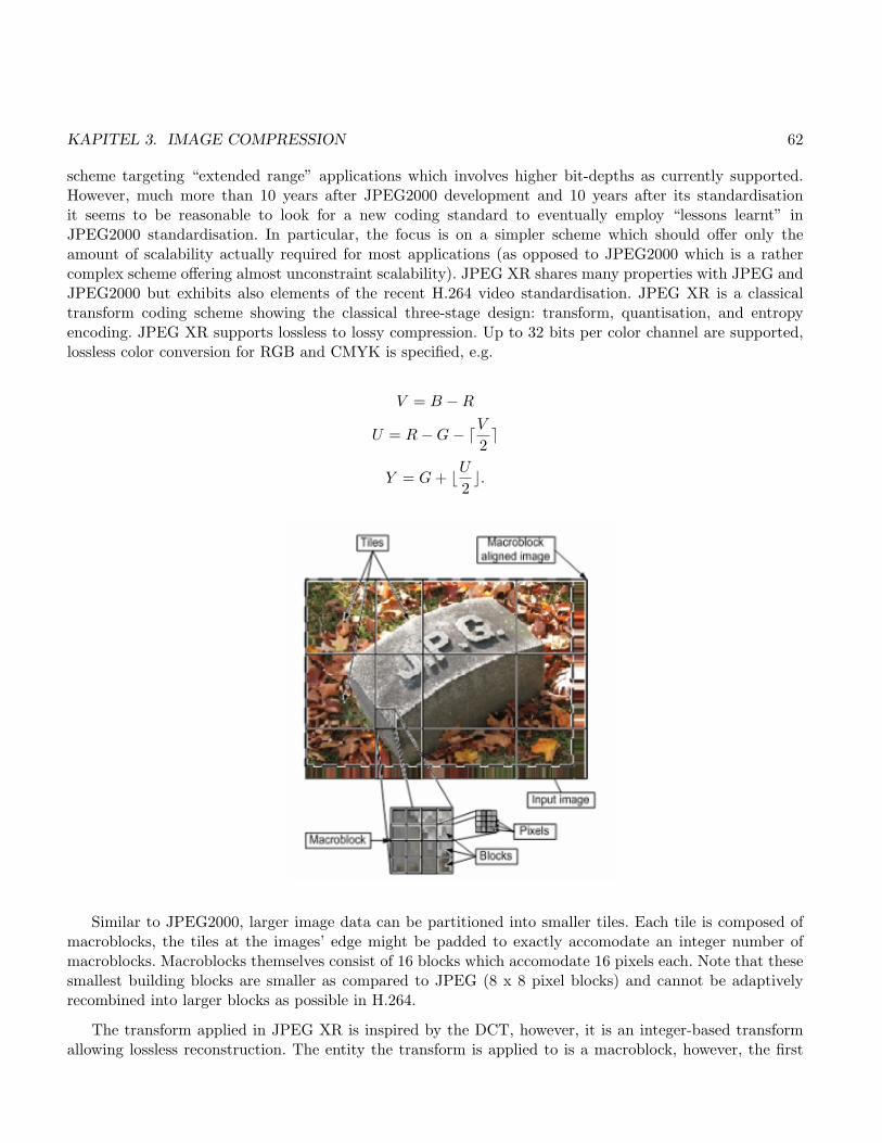
KAPITEL 3. IMAGE COMPRESSION 62
scheme targeting “extended range” applications which involves higher bit-depths as currently supported.However, much more than 10 years after JPEG2000 development and 10 years after its standardisationit seems to be reasonable to look for a new coding standard to eventually employ “lessons learnt” inJPEG2000 standardisation. In particular, the focus is on a simpler scheme which should offer only theamount of scalability actually required for most applications (as opposed to JPEG2000 which is a rathercomplex scheme offering almost unconstraint scalability). JPEG XR shares many properties with JPEG andJPEG2000 but exhibits also elements of the recent H.264 video standardisation. JPEG XR is a classicaltransform coding scheme showing the classical three-stage design: transform, quantisation, and entropyencoding. JPEG XR supports lossless to lossy compression. Up to 32 bits per color channel are supported,lossless color conversion for RGB and CMYK is specified, e.g.
V = B −R
U = R−G− dV2e
Y = G+ bU2c.
Similar to JPEG2000, larger image data can be partitioned into smaller tiles. Each tile is composed ofmacroblocks, the tiles at the images’ edge might be padded to exactly accomodate an integer number ofmacroblocks. Macroblocks themselves consist of 16 blocks which accomodate 16 pixels each. Note that thesesmallest building blocks are smaller as compared to JPEG (8 x 8 pixel blocks) and cannot be adaptivelyrecombined into larger blocks as possible in H.264.
The transform applied in JPEG XR is inspired by the DCT, however, it is an integer-based transformallowing lossless reconstruction. The entity the transform is applied to is a macroblock, however, the first
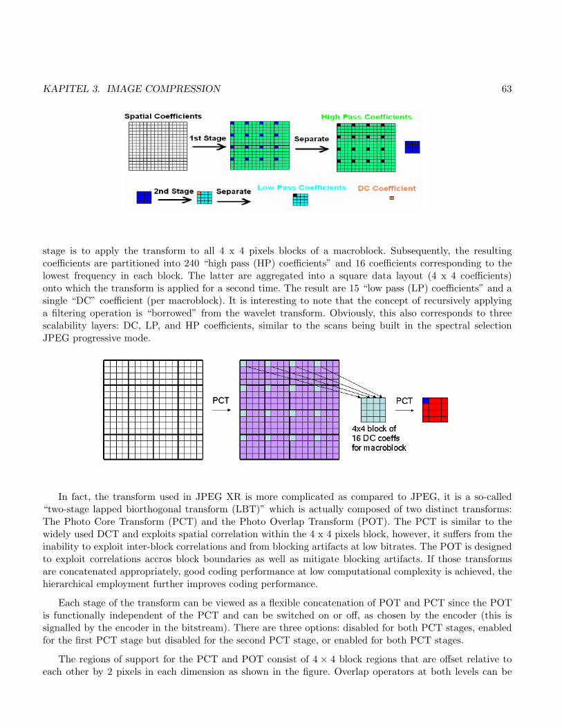
KAPITEL 3. IMAGE COMPRESSION 63
stage is to apply the transform to all 4 x 4 pixels blocks of a macroblock. Subsequently, the resultingcoefficients are partitioned into 240 “high pass (HP) coefficients” and 16 coefficients corresponding to thelowest frequency in each block. The latter are aggregated into a square data layout (4 x 4 coefficients)onto which the transform is applied for a second time. The result are 15 “low pass (LP) coefficients” and asingle “DC” coefficient (per macroblock). It is interesting to note that the concept of recursively applyinga filtering operation is “borrowed” from the wavelet transform. Obviously, this also corresponds to threescalability layers: DC, LP, and HP coefficients, similar to the scans being built in the spectral selectionJPEG progressive mode.
In fact, the transform used in JPEG XR is more complicated as compared to JPEG, it is a so-called“two-stage lapped biorthogonal transform (LBT)” which is actually composed of two distinct transforms:The Photo Core Transform (PCT) and the Photo Overlap Transform (POT). The PCT is similar to thewidely used DCT and exploits spatial correlation within the 4 x 4 pixels block, however, it suffers from theinability to exploit inter-block correlations and from blocking artifacts at low bitrates. The POT is designedto exploit correlations accros block boundaries as well as mitigate blocking artifacts. If those transformsare concatenated appropriately, good coding performance at low computational complexity is achieved, thehierarchical employment further improves coding performance.
Each stage of the transform can be viewed as a flexible concatenation of POT and PCT since the POTis functionally independent of the PCT and can be switched on or off, as chosen by the encoder (this issignalled by the encoder in the bitstream). There are three options: disabled for both PCT stages, enabledfor the first PCT stage but disabled for the second PCT stage, or enabled for both PCT stages.
The regions of support for the PCT and POT consist of 4 × 4 block regions that are offset relative toeach other by 2 pixels in each dimension as shown in the figure. Overlap operators at both levels can be

KAPITEL 3. IMAGE COMPRESSION 64
turned off to minimize ringing artifacts related to long filters, as well as to enable a very low complexitydecoding mode. Overlap operators at both levels can be turned on at very low bit rates to mitigate blockingartifacts.
The PCT and POT are composed of several elementary transforms, out of which the Hadamard transformis the most well known one. All these transforms are integer based, i.e. perfect reconstruction is guaranteedby this design. PCT is almost equivalent to a DCT – when transforming an image by DCT, the inverse PCTgives a very good approximation of the original image and vice versa.
Quantisation is different to JPEG – a common quantisation factor is used for all HP and LP coefficientsinside a macroblock, but these quantisation factors can be different for each macroblock, color bands, andtiles. The quantised value is obtained by dividing the coefficient by the quantisation parameter and roundingto integer. For the lossless mode, quantisation parameter is 1.
Whereas in JPEG only DC prediction is applied, in JPEG XR three types of prediction are applicable:DC prediction, LP prediction, and HP prediction. The DC coefficient of a macroblock (yes, there is only asingle one !) can be predicted in one of the following modes:
• Prediction from left neighbor
• Prediction from top neighbor
• Prediction from left and top neighbors
• no prediction
In order to determine the prediction mode, the differences between the DCs of the top-left and topmacroblocks and those between the DCs of the top-left and left macroblocks are computed. Only in casethe difference in one direction is significantly larger than the other (by a factor of 4), the direction of thesmaller difference is predicted, otherwise prediction from both neighbors is chosen. In case the error is toolarge, no prediction is applied.
The first row or first column of the LP coefficients can be predicted from adjacent macroblocks as well.Options are:
• Prediction of first column from left
• Prediction of first row from top
• no prediction

KAPITEL 3. IMAGE COMPRESSION 65
LP prediction is only applied in case of top OR left prediction of the DC coefficient and matches theprediction direction (and only in case the quantisation parameter of the involved macroblocks matches). Inall other cases there is no LP prediction from adjacent macroblocks.
The first row or first column of HP coefficients in each block is predicted in HP prediction. Options areidentical to LP prediction, however it has to be noted that HP prediction is only applied from the blocks inthe same macroblock. If an individual block does not have a neighbor in the direction specified by predictionmode, no prediction is performed for that block.
For each macroblock, the HP prediction mode is derived from the energy of the LP coefficients of thatmacroblock. If the energy of the first column of LP coefficients is much smaller than the energy of the firstrow of LP coefficients, prediction from top is chosen as the HP prediction mode. If the energy of the first rowof LP coefficients is much smaller than the corresponding energy of the first column, prediction from left ischosen. Otherwise, no prediction is performed. The energy of the LP coefficients in the chroma channel isalso used in deriving HP prediction mode.
Contrasting to JPEG, there is no fixed pattern to scan the 2-D coefficient array into a 1-D vector butadaptive coefficient scanning is applied. In the figure the initial scan patterns for LP and HP coefficients(horizontal) and HP (vertical), respectively, are shown.
Scan patterns are adapted dynamically based on the local statistics of coded coefficients. Coefficientswith higher probability of non-zero values are scanned earlier, i.e. the corresponding scan order is adapted.
This is done by successively updating lists where the number of non-zero values is recorded and wherethe coefficients are sorted in decreasing order according to the number of observed non-zero values. As soonas the ordering get incorrect locally, a local bubble-sort exchange between two coefficients’ positions takes

KAPITEL 3. IMAGE COMPRESSION 66
place. Note that the decoder needs to be in synch (has to generate the same statistical information duringdecoding) to be able to perform the corresponding operations.
The entropy coding stage has also some similarities to techniques in JPEG, however, also here the conceptof adaptivity is used. At first, it is observed that coefficient data can be partitioned into most significantbits and bits of lower significance as shown in the figure. The entropy of the more significant bits is low andthese can be efficiently encoded using a VLC. On the other hand, the bits with lower significance exhibita rather high entropy (they are somewhat close to noisy data as we already know) so that VLC does notwork well and FLC is applied. These data is termed “Flex Bits”.
The entire process is termed “adaptive coefficient renormalisation” and is pretty similar to the JPEGconcept of category and index in the category, but in JPEG XR these data are separated and not encoded inadjacent manner. The actual VLC encoding is done by coding the coefficient “category” and trailing zerosfor all but the first coefficient, where also preceeding zero-runs are recorded, and the last coefficient, wherea “last” symbol is coded. Different tables are used depending on the required categories and and switched
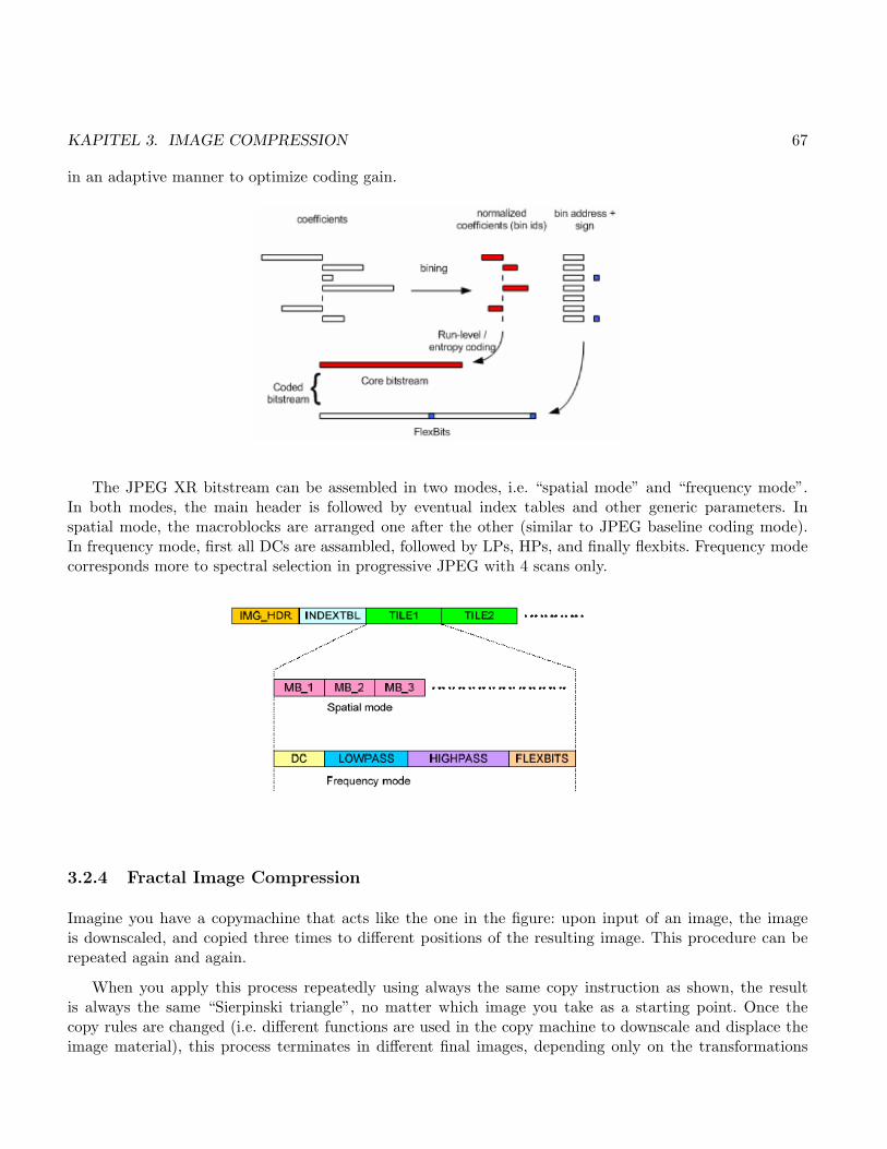
KAPITEL 3. IMAGE COMPRESSION 67
in an adaptive manner to optimize coding gain.
The JPEG XR bitstream can be assembled in two modes, i.e. “spatial mode” and “frequency mode”.In both modes, the main header is followed by eventual index tables and other generic parameters. Inspatial mode, the macroblocks are arranged one after the other (similar to JPEG baseline coding mode).In frequency mode, first all DCs are assambled, followed by LPs, HPs, and finally flexbits. Frequency modecorresponds more to spectral selection in progressive JPEG with 4 scans only.
3.2.4 Fractal Image Compression
Imagine you have a copymachine that acts like the one in the figure: upon input of an image, the imageis downscaled, and copied three times to different positions of the resulting image. This procedure can berepeated again and again.
When you apply this process repeatedly using always the same copy instruction as shown, the resultis always the same “Sierpinski triangle”, no matter which image you take as a starting point. Once thecopy rules are changed (i.e. different functions are used in the copy machine to downscale and displace theimage material), this process terminates in different final images, depending only on the transformations

KAPITEL 3. IMAGE COMPRESSION 68
being applied, but not on the starting image. The copy machine simple means that the transformations areapplied to a start image iteratively.
The transformations involved typically are affine transforms of the form given in the figure where (ei, fi)represent a translation vector and (ai, bi, ci, di) form a matrix which is responsible for scaling / rotating/ flipping the data. For example, the three transformations in the initial copy machine are defined by:ai = di = 1/2, bi = ci = 0, (which means that the matrix is identical for all three but the translation vectoris different), e1 = f1 = 0, e2 = 0, f2 = 1/2, e3 = f3 = 1/2.
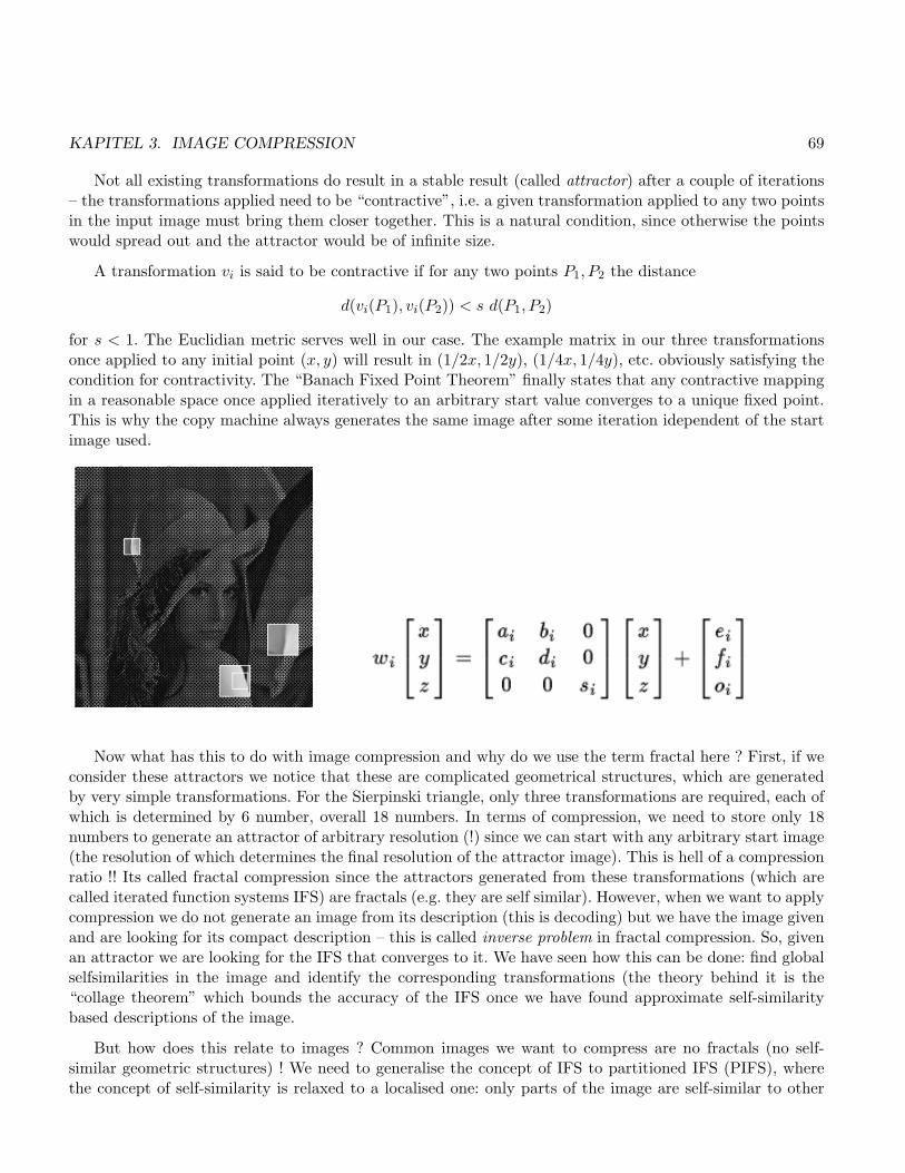
KAPITEL 3. IMAGE COMPRESSION 69
Not all existing transformations do result in a stable result (called attractor) after a couple of iterations– the transformations applied need to be “contractive”, i.e. a given transformation applied to any two pointsin the input image must bring them closer together. This is a natural condition, since otherwise the pointswould spread out and the attractor would be of infinite size.
A transformation vi is said to be contractive if for any two points P1, P2 the distance
d(vi(P1), vi(P2)) < s d(P1, P2)
for s < 1. The Euclidian metric serves well in our case. The example matrix in our three transformationsonce applied to any initial point (x, y) will result in (1/2x, 1/2y), (1/4x, 1/4y), etc. obviously satisfying thecondition for contractivity. The “Banach Fixed Point Theorem” finally states that any contractive mappingin a reasonable space once applied iteratively to an arbitrary start value converges to a unique fixed point.This is why the copy machine always generates the same image after some iteration idependent of the startimage used.
Now what has this to do with image compression and why do we use the term fractal here ? First, if weconsider these attractors we notice that these are complicated geometrical structures, which are generatedby very simple transformations. For the Sierpinski triangle, only three transformations are required, each ofwhich is determined by 6 number, overall 18 numbers. In terms of compression, we need to store only 18numbers to generate an attractor of arbitrary resolution (!) since we can start with any arbitrary start image(the resolution of which determines the final resolution of the attractor image). This is hell of a compressionratio !! Its called fractal compression since the attractors generated from these transformations (which arecalled iterated function systems IFS) are fractals (e.g. they are self similar). However, when we want to applycompression we do not generate an image from its description (this is decoding) but we have the image givenand are looking for its compact description – this is called inverse problem in fractal compression. So, givenan attractor we are looking for the IFS that converges to it. We have seen how this can be done: find globalselfsimilarities in the image and identify the corresponding transformations (the theory behind it is the“collage theorem” which bounds the accuracy of the IFS once we have found approximate self-similaritybased descriptions of the image.
But how does this relate to images ? Common images we want to compress are no fractals (no self-similar geometric structures) ! We need to generalise the concept of IFS to partitioned IFS (PIFS), wherethe concept of self-similarity is relaxed to a localised one: only parts of the image are self-similar to other

KAPITEL 3. IMAGE COMPRESSION 70
parts of the image data, transformations are only applied to parts of the image. All parts of the imageare generated by transformations, the set of all transformations is called PIFS. In order to converge to anattractor, the PIFS needs to be contractive of course. In terms of the copy machine, for each transformationonly a specific part of the image is accessible, the other parts are covered.
When treating images, it gets obvious that not only geometric simlarity is important but also gray scalesimilarity. Therefore, in the transforms used for grayscale images also gray scales are manipulated as shownin the figure (where (x, y) are the spatial coordinates and z is the grayscale): si is a multiplicative factorcontroling contrast and oi is an additive element controling brightness. In terms of the original geometricaltransformation vi we may state that this map defines how the partitioned domains of an original are mappedto the copy, while oi and si determine contrast and brightness modification of the transform.
Now having seen what PIFS mean in the context of images, we are facing the inverse problem whenwe want to compress an image with the fractal technique. In the following we describe how the localtransformations are found given an image to be compressed.
We take two copies of the image, one of which is downscaled to a quater of the original size. Subse-quently, we partition both images into equal-sized tiles: the first copy, having original size, is tiled intonon-overlapping blocks (the ranges), while the second copy can have non-overlapping, highly overlapping,or arbitrary organised tiles (the domains) of the same size (note that due to downscaling, the correspondingareas in the original images have four times the size).
In order to solve the inverse problem, we need to find for each range a transformation in side the image,where the range is the corresponding attractor (we want to generate the range as part of the image by anIFS). When having done this for all ranges, the set of all IFS constitutes the PIFS we are looking for, i.e.each range can be generated by a transformation.
For each range, we look through the set of all domains (the downscaling has already shrunk the corre-sponding areas such that the transformation is contractive anyway) by considering all 8 isometries for eachdomain (rotations and mirrored rotations), for each isometry optimizing oi and si.
Given two squares containing n pixel intensities d1, . . . , dn (domain pixels) and r1, . . . , rn (range pixels),the aim is to select oi and si to minimize the quantity
Ri =n∑
j=1
(sidj + oi − rj)2 .
The minimum is attained when the partial derivatives with respect to oi and si are zero, which occurs

KAPITEL 3. IMAGE COMPRESSION 71
when
si =
n2(n∑
j=1
djrj)− (n∑
j=1
dj)(n∑
j=1
rj)
/n2
n∑j=1
d2i − (
n∑j=1
di)2
and
oi =
n∑j=1
ri − si
n∑j=1
di
/n2 .
So we get an Ri for each domain and select the domain with the smallest value. What do we need tostore per range to be able to generate it as an attractor of the corresponding transformation: the position(or the index) of the domain and its isometry (which gives the geometrical part of the transform since thedownscaling already provides contractivity) and the computed values for oi and si.
Decoding is a very simple procedure: we simply apply the transformations stored to an arbitrary startimage until convegence has been reached, usually not more than 10 iterations are required for decoding.
So far, there is no way to control quality or bitrate apart from the selection of the size of the ranges(large ranges will lead to high compression ratio but low quality). We can apply a threshold to the bestRi found for a range: if the error is too high, we not store the transformation parameters but partitionthe range into its four quadrants and put them on a “waiting list”. After all ranges of the inital range-sizehave been processed, also the domain-pool is partitioned into according smaller tiles and the process isrepeated. Again, there may be a threshold used for controling quality and already partitioned ranges maybe partitioned further. It has to be noted that one partitioning increases the bitrate for a range by a factorof four, since four instead of one transformations (and their parameters) need to be stored. If ranges get

KAPITEL 3. IMAGE COMPRESSION 72
very small, it is less expensive to store them directly instead of storing transformations. Of course, oi andsi can be subjected to quantisation reducing the bitrate.
Quadtree partitioning leads to blocking artifacts mainly in homogeneous areas in case edges cross blockborders. Therefore, other partitioning schemes have been developed which are better able to adapt to edgedirections like the HV and triangulation based schemes. However, the coding cost for domain informationincreases with more complex partitioning schemes.
The coding quality (rate / distortion quality of fractal coding is typically superior to JPEG at low bitratesbut inferior at high bitrates. When compared to JPEG2000 or JPEG XR, fractal coding is inferior acrossthe entire range of possible bitrates. Therefore, it is hard to come up with sensible application scenarios.On eof the most interesting aspects is that of fractal interpolation. As decoding a fractal file can be donewith virtually arbitrary resolution data, the decoding process generates a huge amount of artificial “fractaldata” which is of highly non-linear nature and looks quite pleasing as compared to standard intrapolationtechniques due to the inherent irregularity. ANother interesting aspect is the high decoding speed.
Fractal compression suffers from very high encoding runtime, it is highly assymetric and therefore onlysuited for retrieval-based applicaitons. The complexity of encoding is determined by the amount of overlap-
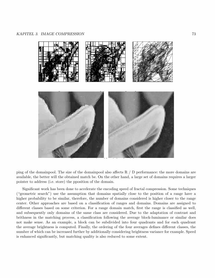
KAPITEL 3. IMAGE COMPRESSION 73
ping of the domainpool. The size of the domainpool also affects R / D performance: the more domains areavailable, the better will the obtained match be. On the other hand, a large set of domains requires a largerpointer to address (i.e. store) the pposition of the domain.
Significant work has been done to accelerate the encoding speed of fractal compression. Some techniques(“geometric search”) use the assumption that domains spatially close to the position of a range have ahigher probability to be similar, therefore, the number of domains considered is higher closer to the rangecenter. Other approaches are based on a classification of ranges and domains. Domains are assigned todifferent classes based on some criterion. For a range domain match, first the range is classified as well,and subsequently only domains of the same class are considered. Due to the adaptation of contrast andbrithness in the matching process, a classification following the average block-luminance or similar doesnot make sense. As an example, a block can be subdivided into four quadrants and for each quadrantthe average brightness is computed. Finally, the ordering of the four averages defines different classes, thenumber of which can be increased further by additionally considering brightness variance for example. Speedis enhanced significantly, but matching quality is also reduced to some extent.
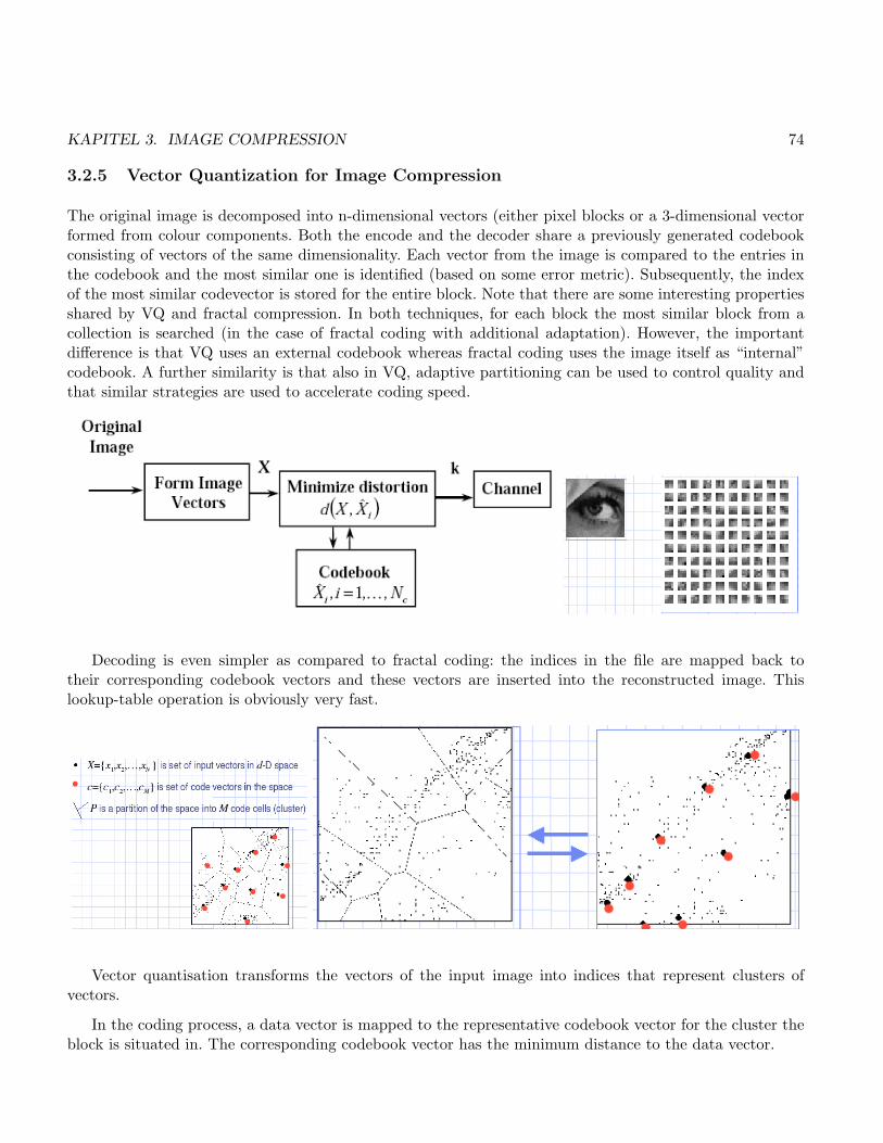
KAPITEL 3. IMAGE COMPRESSION 74
3.2.5 Vector Quantization for Image Compression
The original image is decomposed into n-dimensional vectors (either pixel blocks or a 3-dimensional vectorformed from colour components. Both the encode and the decoder share a previously generated codebookconsisting of vectors of the same dimensionality. Each vector from the image is compared to the entries inthe codebook and the most similar one is identified (based on some error metric). Subsequently, the indexof the most similar codevector is stored for the entire block. Note that there are some interesting propertiesshared by VQ and fractal compression. In both techniques, for each block the most similar block from acollection is searched (in the case of fractal coding with additional adaptation). However, the importantdifference is that VQ uses an external codebook whereas fractal coding uses the image itself as “internal”codebook. A further similarity is that also in VQ, adaptive partitioning can be used to control quality andthat similar strategies are used to accelerate coding speed.
Decoding is even simpler as compared to fractal coding: the indices in the file are mapped back totheir corresponding codebook vectors and these vectors are inserted into the reconstructed image. Thislookup-table operation is obviously very fast.
Vector quantisation transforms the vectors of the input image into indices that represent clusters ofvectors.
In the coding process, a data vector is mapped to the representative codebook vector for the cluster theblock is situated in. The corresponding codebook vector has the minimum distance to the data vector.

KAPITEL 3. IMAGE COMPRESSION 75
VQ can be used to tailor the codebook to a specific application context. For this purpose, a set of trainingvectors (representing the target application context) is used to construct a corresponding codebook. Themost prominent algorithm is the “Linde-Buzo-Gray (LBG)” procedure. We start with a set of trainingvectors, some initial codebook, a distortion measure d, and a fractional distortion change threshold ε. Weset the iteration counter I to 1 and initialize the average distortion over all training vectors D0 to a largenumber. If DI−1−DI
DI−1 ≤ ε, the algorithm terminates. Subsequently the codebook is updated by replacingthe codevector of each decision region (which is the region containing the trainingsvectors that have beenmapped to a single codevector) by a codevector that minimizes the quantisation error of that region. ForMSE, the centroid (average) of the training vectors is that vector.
The centroid is found by computing the mean of the corresponding components of the training vectors.Now we increase the iteratin counter and re-evaluate the above termination criterion. A fundamental issuefor this algorithm is the design of the initial codebook. This can be done by starting right away with arandom codebook of the desired size or by applying the “splitting” techniques which starts with the overallcentroid of the trainingsset, which is split into two parts, applied the LBG algorithm, splits again and so onuntil the desired size of the codebook is reached.
By analogy to fractal compression there exist several techniques to accelerate the encoding process likeclassified VQ or tree structured codebooks. Also many variants exist like mean/residual VQ (after theformation of image blocks the mean is computed for each block and stored in quantised manner (using eg.

KAPITEL 3. IMAGE COMPRESSION 76
DPCM); the quantsed means are substracted from the corresponding image vectors to yield a residual vectorwith zero mean, which is processed with VQ using a suited residual codebook) or interpolative / residual VQ(which is similar to the technique described before except that instead of the mean, a severely downsampledversion of the block is stored and interpolation is used instead of the replication of the mean over the entireblock).
VQ never made it into still image standardisation due to the significant assymetry of the process andthe lower R / D performance as compared to competitors.
3.2.6 Block Truncation Coding
An image is divided into squared blocks of some fixed size (typically 4× 4 pixels in non-adaptive schemes.For each block, the mean x and standard deviation σ is computed. The idea is to construct a compressionscheme which preserves mean and standard deviation on a block basis. A two level quantiser is designedwhich sets all pixels to 1 which are larger than the mean, the others are set to 0. The number of pixels inthe block is m, the number of pixels larger than the mean is q. The bitplane is stored together with themean x and standard deviation σ.
Reconstruction is done by setting all 1’s to a value b and all 0’s to a, which guarantees the abovementionedpreservation:
a = x− σ
√q
m− qand b = x+ σ
√m− q
q
Absolut moment BTC is a variant which replaces the standard deviation by the first absolute centralmoment (which is the sum of the absolute differences from the mean, devided by the number of pixels),which is then preserved together with the mean.
Similar to fractal coding and VQ, BTC can be used in an adaptive manner by starting with a largerblock size and in case of too large errors block partitioning is applied. BTC is very fast but not competitivein terms of R / D performance.

Kapitel 4
Video Compression
In video compression there are no dedicated techniques which allow for lossless compression. Therefore, wedo not discuss lossless techniques here. In video data, we have additional temporal correlation which can beexploited (of course, video frames samples at 60 frames per second tend to be highly similar which calls forexploitation). However, not all techniques / standards do actually support exploitation of the third dimensionby inter-frame compression techniques but support only intra frame compression. These techniques will bedescribed first.
The figure describes major standards as issued by the two major standardasation bodies in the area,i.e. ISO/IEC MPEG (responsible mainly for the entertainment industry) and ITU-T (international tele-communication union, responsible for telecommunication industry). Standardisation started in 1985. It isclearly visible that the work on a single standard can extend over a significant amount of years. In mostcases, standards are completed part by part and several amendments are issued before a standard is actuallycompleted. The so-called “Joint Video Team” (JVT), a joint effort of ISO and ITU-T, is responsible for thelatest standardisation in the area (H.264 / MPEG-4 AVC and SVC).
The different standards have not only been developed at different points in time, they have also dif-ferent target application areas. The figure compares application areas and target bitrates. Only the more
77

KAPITEL 4. VIDEO COMPRESSION 78
recent standards are meant to cover a wider range of bitrates (and application domains). This is usuallyaccomplished by introducing the concept of profiles and levels in MPEG-2,4.
To illustrate the need for compression of video data, let us consider HDTV: with 1080 lines having 1920pixels each at a frame rate of 60 frames / sec in three colour bands this results in 337 Mbytes/sec. Obviously,this calls for a reduction of the bitrate.
4.1 Motion JPEG and Motion JPEG2000
MJPEG and MJPEG2000 perform a frame-by-frame compression of video data (intra-frame compressi-on) and provide synchronisation structures for associated audio. While being inferior in terms of achievedcompression ratio to dedicated video coding standards, these technqiues are required in application whererandom access is needed for each single frame (e.g. video editing applications). MJPEG2000 is of course ca-pable of performing lossless compression due to the corresponding capabilities of the JPEG2000 compressionengine. The Digital Cinema Initiative (DCI) employs MJPEG2000 due to its higher quality as compared toother standards, the higher bitrate is simply not important in its application domain.
4.2 MPEG-1
MPEG stands for “motion picture experts group”, a ISO standardisation body resonsible for standardisationin the area of video entertainment systems. While being most well known in the area of video compression(MPEG-1,-2,-4), also standards in the area of multimedia metadata descriptions for searching multimedialcontent (MPEG-7) and in the area of protection and adaptation of multimedia items (MPEG-21) have beendeveloped.
MPEG-1 (ISO 11172) consists of 5 main parts: systems (multiplexing audio and video and representationof time information for synchronisation), video (which is described in the following), audio (which is coveredin the audio chapter), compliance (specification of test procedures to test compliance of decoders to parts1,2,3), and technical report (including software simulations of parts 1,2,3). The main media target wasstorage of audio and video at 1.5 Mbits / sec on CD-ROM.

KAPITEL 4. VIDEO COMPRESSION 79
MPEG-1 simultaneously supports intraframe and interframe compression. It is restricted to progressivevideo (classical frame-by-frame video in full resolution in each frame), 4:2:0 chroma subsampling, and 8bppvideo data (per colour channel). The satndard syntax supports DCT, motion-compensated prediction, quan-tisation, and VLC. It is important to note that MPEG-1 does not standardise the encoder (here flexibility ispossible plugging in recent improvements and developments and new algorithms) but the bitstream and thedecoder. For example, motion estimation is not standardised at all (although in almost all encoders, blockmatching is used).
There are three different compression modes for the frames of an image sequence:
• Intraframe compression: frames marked by I (I-frames) are strictly intraframe compressed. Theseframe serve as random access points to the sequence and can be decoded without any reference toother frames.
• Interframe compression:
– frames marked by P (P-frames) are encoded relative to the closest I-frame or P-frame in the past.Motion vectors and prediction errors are coded. If motion estimation fails, blocks in P-frames canbe encoded in I-frame mode.
– frames marked by B (B-frames) are encoded relative to two frames, one in the past, one in thefuture, bing either P- or I-frames. If motion estimation fails, blocks in P-frames can be encodedin I-frame mode.
Both P- and B-frames cannot be decoded independently.
The relative number of I, P, and B frames depends on the target compression rate, nature of the content,and access and coding delay requirements. A group of pictures (GOP) ontains a single I frame, and anarbitrary number of P and B frames. The maximal size of a GOP is constrained to 132. There are severalpossibilities for GOP structures, e.g. ....... I I I I I I I ......., ............ I B B P B B I B B P B B I ........., .......IP I P I P I P I P ........... etc.
An entity not existing in JPEG but very important in MPEG are macroblocks: a macroblock consists of4 8× 8 pixels block luminance data and 2 (one for each chroma channel) 8× 8 pixels chroma data.

KAPITEL 4. VIDEO COMPRESSION 80
I Frames are compressed in similar manner as JPEG; the DCT is applied to 8 × 8 pixels blocks,quantisation is applied based on a quantisation matrix (can be user defined) which is scaled to control datarate and quality. Quantisation is followed by a zig-zag scan and a runlength / Huffman coding procedure(also based on tables which can be user defined). Redundancy among quantised DC coefficients is reducedvia DPCM, coded data is separated into luminance and chrominance data.
There is one important difference as compared to JPEG: the strength of quantisation can be different ona macroblocklevel and the corresponding scale factor (MQUANT) is stored in the macroblock header. Thisvalue can be set according to spatial activity of the block or the buffer status in constant bitrate applications.
Interframe coding is based on motion-compensated prediction which consists of a motion estimationprocess which is followed by motion compensation. The most natural idea for exploiting temporal correlationis to compute the difference between adjacent frames and to only encode the difference plus addiitonalreference frames. However, this strategy fails in case of moving objects or camera movement since in thesesituations significant errors are introduced. The basic idea to resolve this issue is to estimate the motion thathas occured between the two frames considered, i.e. in case of a moving object to estimate its displacement.Once the movement is known (encoded in a displacement or “motion vector”), we can predict the luminancesignal within the moving object and incorporate this knowledge into the computation of the difference:the frame to be coded is predicted based on the luminance signal of a reference frame plus the motioninformation, the predicted frame is then substracted from the frame to be coded and this difference isencoded.
Motion-compensated prediction is done on the basis of macroblocks. Motion vectors are assumed to beconstant across a macroblock (small scale motion is neglected as a consequence). Thus, a common motionvector is estimated and assigned to an entire macroblock (for both the luminance and chroma data). For Bframes, two motion vectors are computed and stored for each macroblock. Motion vectors are encoded usingDPCM.
In the following, the process of block matching is described which is a common choice for computingmotion vectors. However, only the usage of motion vectors is standardised and any appropriate algorithmcan be used to compute them (this is where recent technology can be plugged in).

KAPITEL 4. VIDEO COMPRESSION 81
For each macroblock in the current frame (which is to be coded), a squared search window in the referenceframe (which is an already encoded and decoded frame to avoid drift; note that the decoder never has accessto an original frame, which is why the scheme is based on a reconstruction) is centered at the same position.Then, the block in the search window most similar to the block in the current frame is search by comparingthe block to all blocks in the search window (full search). The displacement of the found block to the centerof the search window (which is the position of the block in the frame to be coded) is represented by themotion vector. The criterion to find the most similar block requires some error criterion which is usually thesum of absolute pixel differences (SAD) due to the required high speed of the process. Note the similarityto the encoding algorithms in VQ and fractal compression.
After the most similar blocks in the reference frame have been identified for all macroblocks in thecurrent frame, the predicted frame is constructed by pasting the identified blocks from the reference frameto the position as indicated by the motion vectors – this is the motion compensated prediction, a predictionto the current frame based on pixel data of the reference frame taking “motion” into account. Subsequently,the difference between the current frame and the predicted frame is computed and compressed togetherwith the motion vector field (where the latter is encoded losslessly with DPCM). The compression of the
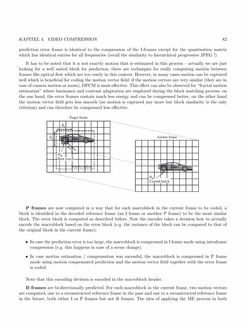
KAPITEL 4. VIDEO COMPRESSION 82
prediction error frame is identical to the compression of the I-frames except for the quantisation matrixwhich has identical entries for all frequencies (recall the similarity to hierarchical progressive JPEG !).
It has to be noted that it is not exactly motion that is estimated in this process – actually we are justlooking for a well suited block for prediction, there are techniques for really computing motion betweenframes like optical flow which are too costly in this context. Hovever, in many cases motion can be capturedwell which is beneficial for coding the motion vector field: if the motion vectors are very similar (they are incase of camera motion or zoom), DPCM is most effective. This effect can also be observed for “fractal motionestimation” where luminance and contrast adaptation are employed during the block matching process: onthe one hand, the error frames contain much less energy and can be compressed better, on the other handthe motion vector field gets less smooth (no motion is captured any more but block similarity is the onlycriterion) and can therefore be compressed less effective.
P frames are now computed in a way that for each macroblock in the current frame to be coded, ablock is identified in the decoded reference frame (an I frame or another P frame) to be the most similarblock. The error block is computed as described before. Now the encoder takes a decision how to actuallyencode the macroblock based on the error block (e.g. the variance of the block can be compared to that ofthe original block in the current frame):
• In case the prediction error is too large, the macroblock is compressed in I frame mode using intraframecompression (e.g. this happens in case of a scene change).
• In case motion estimation / compensation was sucessful, the macroblock is compressed in P framemode using motion compensated prediction and the motion vector field together with the error frameis coded.
Note that this encoding decision is encoded in the macroblock header.
B frames are bi-directionally predicted. For each macroblock in the current frame, two motion vectorsare computed, one to a reconstructed reference frame in the past and one to a reconstructed reference framein the future, both either I or P frames but not B frames. The idea of applying the ME process in both
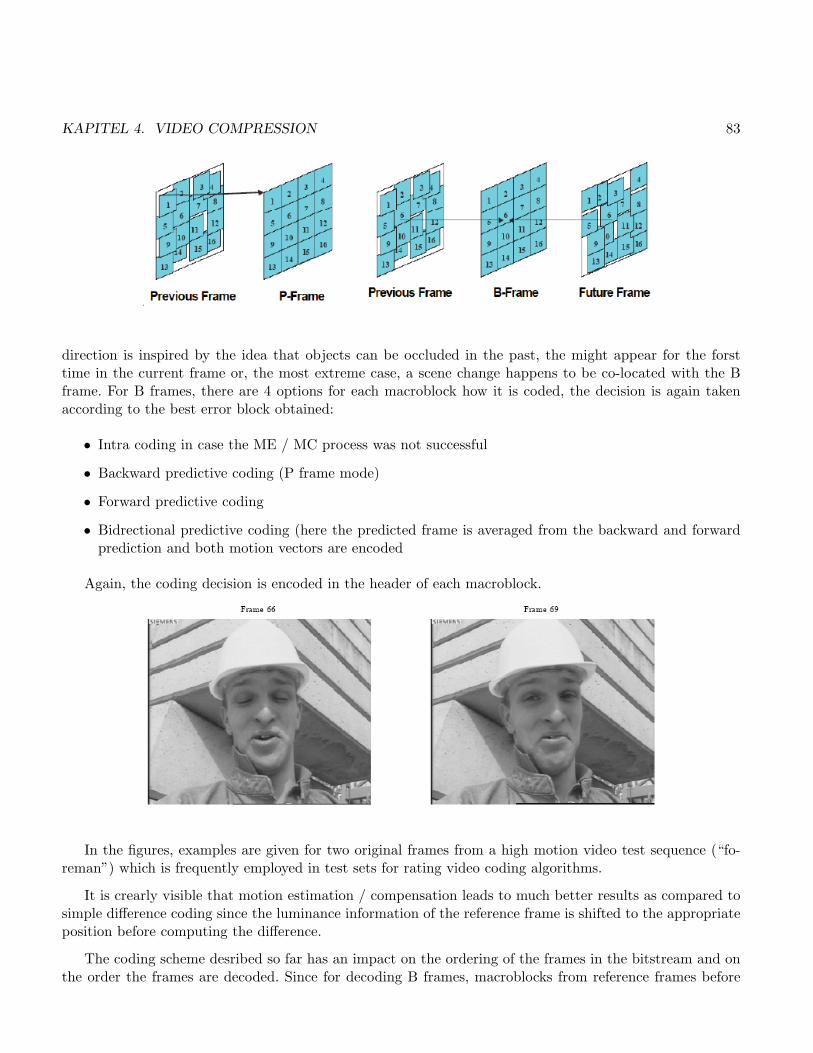
KAPITEL 4. VIDEO COMPRESSION 83
direction is inspired by the idea that objects can be occluded in the past, the might appear for the forsttime in the current frame or, the most extreme case, a scene change happens to be co-located with the Bframe. For B frames, there are 4 options for each macroblock how it is coded, the decision is again takenaccording to the best error block obtained:
• Intra coding in case the ME / MC process was not successful
• Backward predictive coding (P frame mode)
• Forward predictive coding
• Bidrectional predictive coding (here the predicted frame is averaged from the backward and forwardprediction and both motion vectors are encoded
Again, the coding decision is encoded in the header of each macroblock.
In the figures, examples are given for two original frames from a high motion video test sequence (“fo-reman”) which is frequently employed in test sets for rating video coding algorithms.
It is crearly visible that motion estimation / compensation leads to much better results as compared tosimple difference coding since the luminance information of the reference frame is shifted to the appropriateposition before computing the difference.
The coding scheme desribed so far has an impact on the ordering of the frames in the bitstream and onthe order the frames are decoded. Since for decoding B frames, macroblocks from reference frames before

KAPITEL 4. VIDEO COMPRESSION 84
and after a B frame are required for the decoding of the B frame data, these reference data are storedfirst into the bitstram and also decoded in this order. For correct display, the frames have to be re-orderedagain. Note that as a consequence, the ordering of the data in the original video does not correspond to theordering of the data in the bitstream.
The figure shows a block diagram of a typical hybrid motion-compensated predictive video coding scheme.It has to be noted that due to the necessity to base predictions on reconstructed frames, each encoder needs
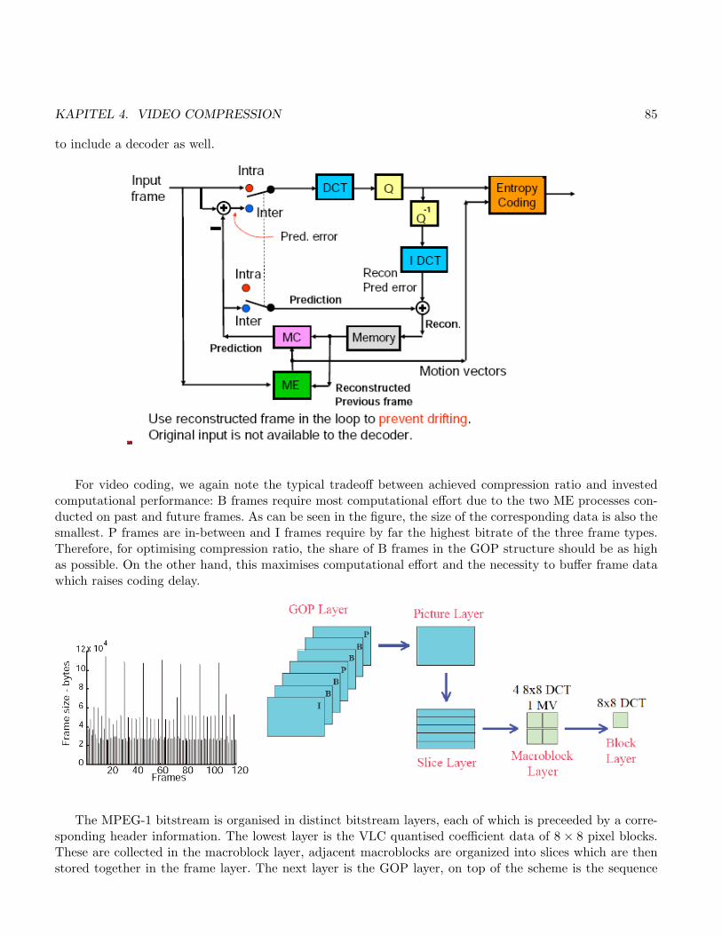
KAPITEL 4. VIDEO COMPRESSION 85
to include a decoder as well.
For video coding, we again note the typical tradeoff between achieved compression ratio and investedcomputational performance: B frames require most computational effort due to the two ME processes con-ducted on past and future frames. As can be seen in the figure, the size of the corresponding data is also thesmallest. P frames are in-between and I frames require by far the highest bitrate of the three frame types.Therefore, for optimising compression ratio, the share of B frames in the GOP structure should be as highas possible. On the other hand, this maximises computational effort and the necessity to buffer frame datawhich raises coding delay.
The MPEG-1 bitstream is organised in distinct bitstream layers, each of which is preceeded by a corre-sponding header information. The lowest layer is the VLC quantised coefficient data of 8 × 8 pixel blocks.These are collected in the macroblock layer, adjacent macroblocks are organized into slices which are thenstored together in the frame layer. The next layer is the GOP layer, on top of the scheme is the sequence

KAPITEL 4. VIDEO COMPRESSION 86
layer which has usually one instance and is preceeded by the main header.
As mentioned before, ME is not standardised and can be conducted in various manners. Full search asdescribed before is very costly in terms of computational effort and especially, in software often differenttechniques are applied, basically reducing the number of blocks in the reference frame search range whichare compared to the block in the current frame. This is usually not done by random subsampling but byfirst using a sparse grid across the entire search window, subsequently refining the grid in the are of thelocal minimum found on the sparse grid. This strategy dramatically reduces search time, on the other handthe global optimum is not often found but in most cases, matches have sufficient quality. The two examplesshow two different search patterns (three step search TSS and cross search), a large variety of other patternshas been investigared in literature.
A different approach to improve motion estimation is to apply a hierarchical model. The advantage isthat in a lower resolution, the process is less affected by noise and chances are better that actual motionis identified. Additionally, computational complexity is reduced in case that the search result in the lowerresolution is taken as local minimum, which is only refinded locally in the higher resolutions.
A final issue not discussed so far but a very important one is that ME and the storage of motion vectorscan be done with half pixel accuracy in MPEG-1. This sounds strange at first sight since there seems to besimply no data between pixels. The idea is that the data in the reference frame can be interpolated betweeninteger pixel positions. This turn out to be highly beneficial since
• simply more data is available to find block matches of high quality (compare domain overlap in fractalcompression) and
• in case of high motion, visual data may simply not be present due to a sampling rate which is too lowfor the amount of motion. Here, the missing data is interpolated by fractional pixel accuracy ME /MC.
Again we face a tradeoff between compression ratio and computaitonal effort since the interpolationof data (usually bilinear interpolation schemes as the one shown in the figure) represents a significantcomputational burden. However, it has turned out that dispite of the higher bitrate required for the motionvectors, fractional pixel ME / MC is highly beneficial and is applied in all future standards not only as anoption but as a must.

KAPITEL 4. VIDEO COMPRESSION 87
Bitrate control is similar to JPEG (based on scaling quantiser matrices) but there are more options inMPEG-1: spatially adaptive quantisation within a frame and frame dropping (reducing the frame rate) canbe applied to B frames since the corresponding data does not serve as reference data for any other frames.
4.3 H.261 and H.263
H.261 is primarily intended for videoconferencing over ISDN channels at rates p× 64 kbits/sec video andaudio combined. This standard is very similar to MPEG-1 but does not define B frames. The reason isthat symmetry of encoding and decoding and avoiding excessive frame buffering and corresponding codingdelay is important for the interactive target applications. A H.261 encoder may skip frames and/or reducespatial resolution to control rate besides adapting quantisation. Chroma sampling is 4:2:0, only QCIF (176×144 pixels luminance resolution) and CIF (common image interchange format, 352 × 288 pixels luminanceresolution) are supported.

KAPITEL 4. VIDEO COMPRESSION 88
H.263 improves compression efficiency to support videoconferencing with 28.8 Kbits/sec over PSTNs(pulic switched telephone networks). Additional image formats are sub-QCIF (128×96 pixels), 4CIF, and 16CIF (the latter two doubling the images’ side length from CIF in each step). Contrasting to H.261, ME canbe done with half pixel accuracy and MV predictive coding is improved from simple difference coding to apredictor based on a median of MV from three neighboring marcoblocks. Arithmetic coding and overlappingmotion compensation (reducing blocking artifacts) can be used optionally. Also, an advanced predictionmode can be used optionally based on prediction of 8× 8 pixel blocks: the prediction is a weighted averageof the MV of the block and the MVs of two neigboring blocks (right and bottom block). Additionally, aresticted form of bidirection prediction can be used (PB frames, only one between two P frames, the unitof P frame – in the future of the B frame – and the B frame is called PB frame).
H.261 belongs to the H.320 familiy of standards where also audio compression, multiplexing, and com-munication protocols are standardised. The same is true for H.263, which belongs to the H.324 family.
H.263+ and H.263++ exhibit many features as finally standardised in H.264 and never have beenaccepted widely.
4.4 MPEG-2
MPEG-2 is intended for higher bitrates and higher quality than MPEG-1 (for DVD, BluRay, DVB, HDTV);this is achieved partially by allowing other types of color subsampling: 4:2:2 where only one dimension issubsampled and 4:4:4 without subsampling).
MPEG-3 was originally intended for HDTV but has been incorporated into MPEG-2 as a “profile”.Several profiles and levels have been defined supporting different functionalities (profiles) and parameterranges (level). As a consequence, there is not a single MPEG-2 “algorithm” but many different algorithmsfor the different profiles. This makes the situation more difficult since a decoder needs to support the profilea bitstream has been generated with at the encoder.
MPEG-2 (ISO 13818) is published in 7 parts: multiplexing, video, audio, conformance testing, technical

KAPITEL 4. VIDEO COMPRESSION 89
report with software simulation, digital storage media command control (DSM-CC, for VoD applicationsdefining protocols for manipualtion / playback of MPEG bitstreams, and a non-backward compatible audiocompression scheme (AAC as known from i-Tunes).
The basic structure and core coding system of MPEG-2 is similar to MPEG-1, and a MPEG-1 video withso-called constrained parameters can be decoded by any MPEG-2 decoder (a flag in the MPEG-1 bitstreamindicates this property: ≤ 768 × 576 pixels, frame rate maximal 30 fps, bitrate at most 1.856 Mbits / sec(constant bitrate)). However, there are also important differences which will be discussed in detail in thefollowing:
• MPEG-2 is intended for higher quality and higher bitrate (half pixel accuracy for MV is a must, finercoefficient quantisation, separate quantisation matrices for luma and chroma for 4:4:4 and 4:2:2 data),
• introduction of interlaced video (fields instead or frames in progressive video),
• corresponding modes in ME / MC,
• scalable profiles, and
• error resilience and error concealment
Interlaced video (as opposed to “progressive” video) is composed of fields. Each field consists only ofeven or odd numbered lines (even and odd filed) and in each field all pixels values correspond to the samepoint in time, however, two fields are displaced by a certain amount of time. This scheme originates fromearly TV, where upon arrival of new data (a field), only half of the lines in the image needed to be refreshed.This leads to new data entities with respect to compression as compared to progressive video: interlaceddata can be either compressed as “field pictures” (where each field is compressed as an idenpendent unit)or as “frame pictures” (where the corresponding lines of two fields are interleaved and compressed together.
The decision about how to encode pictorial data can be made adaptive to image content and rate-distortion considerations and can be mixed within an image sequence as shown in the figure. This mixture

KAPITEL 4. VIDEO COMPRESSION 90
is not arbitrary, i.e. if the first field of a frame is a P (B) picture, then also the second field should be P (B).If the first field is I, the second should be I or P.
Due to the reduced horizontal correlation present in field pictures (which is due to the reduced resolutionin this direction, basically a downsampling by 2 operation is done) an alternate scan pattern is used aftertransform and quantisation as shown in the figure.
Due to the introduction of field and frame pictures, the motion estimation and compensation processcan offer more flexibility and more modes to exploit temporal correlations. For field pictures, field-basedprediction can be done by computing a single motion vector per macroblock in each direction or by computingtwo motion vectors in each direction (two MV for each field using two fields as reference). Dual primeprediction (see below) is different.
For frame pictures, a frame-based prediction can be done, where one MV is computed per macroblock ineach direction (the fields of the reference frame may have been compressed individually as two field pictures

KAPITEL 4. VIDEO COMPRESSION 91
or together as a frame picture). Field-based prediction in frame pictures (as shown in the figure) computestwo motion vectors per marcoblock for each prediction direction, one MV for each of the fields. Again, thefields of the reference frames can be compressed individually or together.
A specific case of prediction is “dual-prime” prediction. For field pictures, data from two reference fieldsof opposite parity is averaged to predict a field picture. A single MV is computed for each macroblock ofthe field. This motion vector V points to the reference field. The second MV, V1, pointing to the field ofother parity, is derived from V on the assumption of a linear motion trajectory (i.e. no acceleration). Theprediction a is subsequently averaged between b and c. This mode is restricted to P pictures in case thereare no B pictures between predicted and refereced fields.
In frame pictures, dual prime prediction is a special case of field-based prediction. A single MV V iscomputed for each macroblock of the predicted frame picture. Using this vector, each field in the macroblockis associated with a field of the same parity in the reference frame. Motion vectors V1 and V2 are derivedfrom V based on linear motion trajectory assumption again. Predictions for a and b are based on averagingc, e and d, f , respectively.
In frame pictures, it is possible to switch prediction modes on a macroblock basis. For example, theencoder may prefer field-based prediction mode over frame prediction in areas with sudden and irregularmotion, since in this case the differences between even and odd field in predicted and reference frame do notmatch..
The concept of scalability refers to the ability of a decoder to decode only a part of a scalable bitstream

KAPITEL 4. VIDEO COMPRESSION 92
and generate a “useful” video. E.g., a lower resolution video can be obtained without decodeing the entirebitstream first and then lowering the resolution by postprocessing, or without simulcasting two distinctbitstreams corresponding to different resolutions. There are three types of scalability in video coding:
1. Temporal scalbility (different frame rates)
2. Spatial scalability or Resolution scalablity
3. Quality scalability (different levels of SNR / picture quality)
In MPEG-2, scalbility is achieved by the concept of layered compression, i.e. by generating a base layerand additional enhancement layers, which successivley improve the quality of the base layer if decodedtogether. In all schemes of this type, usually a higher computational demand and reduced compressionefficiency is observed as the price of increased functionality.
Temporal scalability is achieved very easily by assigning a set of suited B frames to the enhancementlayer. In order to keep the compression degradation as small as possible, correlations among the frames inthe base layer and those in the enhancement layer need to be exploited. While the first scheme depicted issimilar to the classical prediction in a GOP (here prediction is only from base layer to enhancement layer),the second one applies a different prediciton structure (including intra-enhancement prediction).
Spatial scalability is accomplished in a similar manner as in hierachical JPEG. Video frames are repre-sented as spatial pyramids, prediction for the enhancement-layer frames is done based on base layer data(interpolated from the lower resolution) and based on temporal prediction in the enhancement layer dataitself.

KAPITEL 4. VIDEO COMPRESSION 93
Finally, quality scalability is achieved based on differently quantised version of the video (as opposedto the lower resolution in resolution scalability). The reconstructed lower quality version is used as theprediction for the enhancement layer as well as motion compensated data from the enhancement layer itselfis used. The scalability profiles in MPEG-2 (see below) were not very successful since when using a fewlayers, compression performance is drastically reduced at the price of significant complexity increase.
Since MPEG-2 is also intended for broadcast applications where transmission errors are to be expected(e.g. DVB-T, DVB-S, ....), several techniques how to cope with these errors have been incorporated intothe standard. In particular, “error concealment” strategies have been suggested for the decoder. In P and Bframes, a lost marcoblock is substituted with the motion compensated macroblock of the previously decodedframe. For motion vectors, the MV belonging to the block above the lost macroblock is used. If the topmacroblock used in concealment is intra coded, there are two options:
• If a MV for the intra block has been included (the standard allows to do this for concealment purposes),the concealment is done like described before.
• Otherwise, the concealment is done using the MV of the macroblock of the block in the previous frame(assuming zero motion). For the macroblocks in the first line in a slice, it is done in the same manner.

KAPITEL 4. VIDEO COMPRESSION 94
In I-frames, error concealment is done in the same manner. The scheme can be improved by using twoadjacent macroblocks, in case enough MV are retained, motion-compensated concealment can be done toapproximate the lost macroblock.
Different functionalities are supported by different profiles of the standard, which are basically differentalgorithms. The different levels correspond to different parameter ranges which are supported (e.g. frameresolution, frame rate, etc.). A MPEG-2 decoder does not need to support all profiles and levels, in contrast,usually, a given decoder supports a specific profile and level combination (see the figure for examples).

KAPITEL 4. VIDEO COMPRESSION 95
4.5 MPEG-4
MPEG-4 (ISO/IEC 14496) currently consists of 27 (!) parts out of which we will describe Part 2 (Visual)and later also Part 3 (Audio). MPEG-4 Part 10 is commonly referred to as MPEG-4 AVC (advanced videocoding) or H.264. MPEG-4 is targeted to applications in the multimedia area. Since interactivity is animportant aspect of many multimedia applications, providing this functionality is one of the main aimsof the standard. Due to the frame-oriented processing in former standards, interactivity was very limited.MPEG-4 uses the concepts of (arbitrary shape) video objects instead of frames to enable object-basedinteractivity.
MPEG-4 fuses ideas from the following (successful) fields:
• Digital TV
• Interactive graphics applications (e.g. computer games)
• Interactive multimedia applications (e.g. WWW)
The aim is to improve the applicability for users, service providers, and content creators:
• Content creators: due to object-based representation, parts of the video data can be kept and re-used.Also copyright can be protected in a more focussed manner.
• Service providers: network load can be controlled better due to MPEG-4 QoS descriptors.
• Consumers: facilitating interactivity with multimedia data, over high-bandwidth networks or mobilenetworks.
As a consequence, MPEG-4 does not only provide an improvement with respect to compression butmainly is focused on improved functionality. This is achieved by standardisation in the following areas:
• Representation of “media objects” which are units of visual or audio (or both) data, which can be ofnatural or synthetic origin.
• Composition of media objects to an audiovisual scene.
• Multiplexing and synchronisation of data corresponding to media objects for network transfer accor-ding to respective QoS requirements.
• Interaction between user and audiovisual scene (note that this requires an uplink which does more asFFW or RWD).
MPEG-4 audio-visual scenes are composed of several media objects which are organised in an hierarchicalfashion (tree). The leaves of the tree are “primitive media objects” like still images, video data, audio objects,etc. Additionally, special objects are defined like text, graphics, synthetic heads and faces with associatedtext to synthetise speech in a synchronised manner to head animation (talking head), synthetic sound, etc.
Scene description is standardised (features similar to computer graphics and virtual reality – VRML)and supports the following functionalities:

KAPITEL 4. VIDEO COMPRESSION 96
• media objects can be positioned at any given point in a coordinate system.
• media objects can be transformed thereby changing its geometrical, optical, and acustical appearance.
• primitive media objects can be fused into a larger single media object.
• streaming data can be “applied” to media objects to change their characteristics (e.g. a sound, amoving texture, animation parameter for a face, ....).
• the viewing and listening position can be changed.
Synchronised transmission of streaming data with different QoS over a network is provided employing asynchronisation layer using a two-layer multiplexer.

KAPITEL 4. VIDEO COMPRESSION 97
The first layer of the multiplexer is implemented corresponding to the DMIF (delivery multimedia inte-gration framework) specification. DMIF is a session protocol for multimedia data similar to FTP. Using theMPEG FlexMux tool, elementary streams with identical or similar QoS requirements are treated together.TransMux is used to implement the actual QoS requirements for the fused streams. The standard only coversthe interface to TransMux, the actual deployment has to be carried out using the network protocol.
Interactivity (uplink !) is facilitated by e.g. changing viewing and/or listening angel, remove or translateobjects from / in a scene, trigger a cascade of events by a mouseclick (e.g. playing a video, an animatedgraphics), selection of suited language or selection of the desired view from a multiview video.
4.5.1 Compression of synthetic video objects
To give two examples, we describe face animation and general purpose mesh-coding with texture mapping.
A two-dimensional mesh is a partitioning of a 2-D planar region into polygonal parts. The corner pointsare denoted as “node points” or “vertices”, MPEG-4 only supports a triangulation. A 2-D dynamic meshdescribes the movement of the vertices in a certain amount of time. Efficient coding (based on predictivecoding of course) is defined for those data. In order to map texture onto a 2-D mesh, the triangles of theoriginal mesh are deformed and the texture is adjusted to the resulting parts by a technique called “warping”.In case of restricting the vertices movements to affine mappings, the movement can be stored very efficiently.
A “facial animation object” is a generic 2-D mesh of a face which can be used to generate an animatedsynthetic face. Shape and appearance can be described by “Facial Description Parameters” (FDP). “FacialAnimation Parameters” (FAP) are used to generate facial expressions by manipulating specific mesh points.
MPEG-4 standardises techniques how to efficiently store FDP and FAP and also how to interpolatethem in case of data loss. As in the case of generic 2-D meshes, facial texture (an image of a specific person)can be mapped onto the wireframe model. MPEG-4 defines JPEG2000 as the technique to compress thetextures used for mapping in a scalable manner. The same ideas are used for a parameterised descriptionand animation of the entire human body.
Mesh-representation enables interesting features:
• Augmented reality: mixture of computer-generated data and natural data.
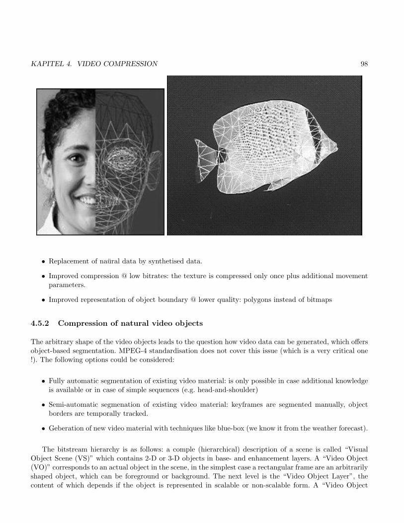
KAPITEL 4. VIDEO COMPRESSION 98
• Replacement of naural data by synthetised data.
• Improved compression @ low bitrates: the texture is compressed only once plus additional movementparameters.
• Improved representation of object boundary @ lower quality: polygons instead of bitmaps
4.5.2 Compression of natural video objects
The arbitrary shape of the video objects leads to the question how video data can be generated, which offersobject-based segmentation. MPEG-4 standardisation does not cover this issue (which is a very critical one!). The following options could be considered:
• Fully automatic segmentation of existing video material: is only possible in case additional knowledgeis available or in case of simple sequences (e.g. head-and-shoulder)
• Semi-automatic segmenation of existing video material: keyframes are segmented manually, objectborders are temporally tracked.
• Geberation of new video material with techniques like blue-box (we know it from the weather forecast).
The bitstream hierarchy is as follows: a comple (hierarchical) description of a scene is called “VisualObject Scene (VS)” which contains 2-D or 3-D objects in base- and enhancement layers. A “Video Object(VO)” corresponds to an actual object in the scene, in the simplest case a rectangular frame are an arbitrarilyshaped object, which can be foreground or background. The next level is the “Video Object Layer”, thecontent of which depends if the object is represented in scalable or non-scalable form. A “Video Object

KAPITEL 4. VIDEO COMPRESSION 99
Plane (VOP)” is a temporal sample of a VO, several VOPs can be grouped to a “Group of Video ObjectPlanes (GOV)”.
VOPs can be compressed in different manners, the classical mode a VOP contains shape information,motion parameters, and texture information. As an alternative, a VOP can be represented as “sprite” (seebelow). Single VO are processed and compressed indenpendent of each other.
Coding of shape information: In case of binary shape information, shape is defined by a binary matrixwhich covers the objects’ shape. The matrix is tiled into 16x16 blocks, the binary alpha blocks BAB, valuesoutside of the object are set to 0, the other values are set to 1. In addition to BABs at the border of theobject, two special types of blocks have all identical values 0 – transparent or 1 – opaque which are encodedby a single symbol. BABs are encoded by motion compensation, arithmentic encoding and DPCM of motionvectors. In case of storing transparency information, gray scales with 8bpp are used instead of binary valuesand DCT-based coding is done instead of AC.
Motion compensation: beside a technique for global motion compensation which computes a MV for eachpixel based on warping a grid the classical ME / MC concept of MPEG is used, only adapted to the VOPconcept. ME is done only for macroblocks, which are situated in a rectangle surrounding the shape of theobject. In case of blocks situated entirely inside the object, there is small difference to MPEG-2 (overlappedME / MC can be used and MV can be computed for each 8x8 block). For macroblocks being positionedonly partially inside the VOP, “modified block (polygon) matching technique” is used, which means thatonly pixel values inside the VOP are used for evaluating the difference; if the reference block is outside theVOP, pixel values are filled according to a fixed scheme.

KAPITEL 4. VIDEO COMPRESSION 100
Texture coding: For texture blocks inside the VOP, compression is conceptually identical to MPEG-2.Blocks positioned at the border of the VOP are pasted with values: for B or P-VOPs, 0 is used for pasting,for I-VOPs the mean of the VOP (with some slight modifications) is used. Alternatively, a shape adaptiveDCT can be used, providing better compression (no pasted values !) but causing more complex computations(hardware support is difficult to achieve). DC and large AC coefficients can be used to predict the coefficientsof the block to be encoded. There are three scan variants (following the prediction of the coefficients): zig-zag,alternate-horizontal and alternate-vertical.
Sprite coding: a sprite is a large VO which is present during an entire scene and which is usually largerthan the current field of view of a single frame. A classical example is a background sprite. A VO like thisis transmitted / decoded at the start of a scene and modified according to the needs of the current frames.Coding a sprite is done as for I-VOPs.
In extending error concealment capabilities of MPEG-2, MPEG-4 is also aimed towards mobile environ-ments and their even more problematic transmission errors:
• Resynchronisation: unique markers are embedded into the bitstream indicating synchronisation pointsfrom which decoding can be restarted.
• Data partitioning: Motion vector data and texture data are separated in order to facilitate moreefficient error concealment. In case one of the two data types is lost, the dislocated other type can be

KAPITEL 4. VIDEO COMPRESSION 101
used for concealment.
• Header extension Code: additional redundant header information is inserted into the bitstream.
• Reversible VLC: codewords have been developed, which can be decoded from both sides. in case thefront part is lost, decoding can start from the end.
Scalability is adapted to the VOP concept. Scalability is implemented by multiple VOL. Scalability onan object basis is achieved by the VOP concept itself in a natural manner. For temporal scalability, twotypes are supported:
• Enhancement layer improves temporal resolution of a part of the base layer only (the important one)
• Enhancement layer improves temporal resolution of the entire base layer

KAPITEL 4. VIDEO COMPRESSION 102
The most well known implementations of MPEG-4 Part 2 are DivX and Xvid, however, they only supportrectangular VOP. There are no implementations and applications which support all functionalities. It seemsthat object-based interactivity is not really required for video consumption.
4.6 H.264 / MPEG-4 AVC
An inofficial experimental coding scheme was named “H.26L” which is still seen in some result charts andpapers. H.264 follows a two layer design: a network abstraction layer (NAL) and a video coding layer (VCL).NAL is designed in order to provide “network friendliness” in the sense of enabling the use of the VCL fora broad variety of systems (e.g. RTP/IP, file formats (ISO MP4), H.32X, DVB-X). The video is organisedin NAL units, each of which is a packet of data preceeded by a header byte indicating the type of data.Data is interleaved with emulation prevention bytes to prevent the “start code prefix” to be generated. Thisdefinition is used for data transport in both packet-oriented and bitstream oriented transport systems.
4.6.1 NAL
For byte-stream format (e.g. video conferencing H.320), the data is transported as an ordered stream

KAPITEL 4. VIDEO COMPRESSION 103
of bytes within which the location of the NAL unit boundaries is identifiable from the start code prefix. Inother systems (e.g. RTP) the coded data is carried in packets that are framed by the transport protocol,so identification of the boundaries of the NAL units can be established without the the start code prefixpatterns. NAL units are classified into VCL units (containing actual video data) and non-VCL units (contai-ning header information like parameter sets or timing information). A parameter set is supposed to containinformation that is expected to change rarely and can be used to decode a significant number of VCL NALunits, sequence and picture parameter sets are distinguished. Each VCL NAL unit contains an identifier tothe relevant sequence and picture parameter sets.
An access unit composed of several NAL units can be decoded to one entire frame – called a primarycoded picture. These data consists of “slices” that represent samples of the video. Additional redundantrepresentations of some areas of the same frame can be included for error concealment purposes – redundantcoded pictures. Decoders are not required to decode these data. If the frame is the last of a coded videosequence (a group of picture that is indenpendently deocidable and refers to a single sequence parameterset) an “end of sequence” NAL unit may be present; if it is the end of the entire NAL unit stream, an “endof stream” NAL unit may be present.
A coded video sequence consists of a series of access units, at the beginning of which an “instantaneousdecoding refresh (IDR)” access unit is found. This IDR access unit contains an intra frame – a frame whichcan be decoded without reference to any other frame in the NAL unit stream. There are no references in thesequence to frames before the IDR access unit. A NAL unit stream may contain one or more coded videosequences.
4.6.2 VCL
The basic idea is identical to former standards since it follows the idea of block-based hybrid video coding,where the video is represented by squared units of data, the macroblocks, consisting of 16x16 samplesluminance with the additional associated chroma samples. Of course there is support for progressive andinterlaced video as it is for MPEG-2,4. It has to be noted that improved coding efficiency is not caused byjust few single new techniques, it is the sum of many smaller enhancements that lead to the gain in R/Dperformance.
Slices are sequences of macroblocks which are processed in raster scan order (except if FMO is used, seebelow). A frame can be split into one or several slices as shown in the figure. Slices are self-contained in thesense that in case of available picture and sequence parameter sets their syntax elements can be parsed fromthe bitstream and the pixel data can be correctly decoded without the use of data from other slices (giventhat correct reference frames are available).
Flexible macroblock ordering (FMO) modifies the way frames are partitioned into slices and macroblocksby using the technique “slice group”. Each macroblock can be assigned to any slice independent of its scan-order position based on the “macroblock to slice group” map (which contains a slice group ID for eachmacroblock). The purpose of doing this can be a region of interest coding type or, like in the example ofthe checkerbord pattern, a tool for error concealment if these two slice groups are transmitted in separatepackets. In addition to the classical I, P, and B slices, SP and SI slices are defined: an SP slice is a so-calledswitching P slice which enables efficient switching between pre-coded pictures of different bitrate. An SIslice is used to enhance an SP slice for a perfect macroblock match to enable random access.

KAPITEL 4. VIDEO COMPRESSION 104
With respect to interlaced video, we again have frame pictures, field pictures, or an adaptive mixture,where for two vertically adjacent macroblocks the decision can be taken how to process them (interleavedor non-interleaved). The choice between the three options can be made adaptively for each frame in thesequence – the choice between the first two is called picture adaptive frame/field (PAFF) coding. The thirdoption is called macroblock adaptive frame/field coding (MBAFF) and is applied in case a frame consistsof areas with high motion and other areas with low motion content. The distinction between PAFF andMBAFF frames leads also to different scan oders, motion vector coding etc. for the two modes. While ingeneral MBAFF is more effieicent in terms of compression due to its adaptivity, for some rare cases likerapid global motion, scene change etc. PAFF can be superior.
Intra-Frame Prediction: In all slice coding types, three different types of intra coding are supported.Intra 4x4 mode, Intra 16x16 mode, and I PCM mode. I PCM mode bypasses prediction and transformcoding and directly encodes the values of the encoded samples (for lossles coding, representation of anomalouspicture content without expansion). Intra-prediction is done in the spatial domain.
When using Intra 4x4 mode each 4x4 pixels block is predicted from spatially neighbouring samples.One out of nine prediction patterns is employed – the way how to choose the most appropriate one is notstandardised and is subject to current research. The aim is to exploit the redundancy of edge-like structures.When utilising Intra 16x16 mode (full macroblock prediction), the whole luma component of a macroblock
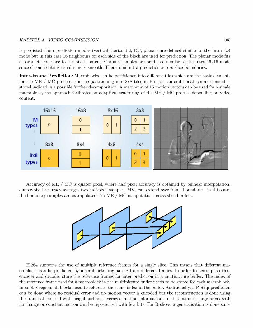
KAPITEL 4. VIDEO COMPRESSION 105
is predicted. Four prediction modes (vertical, horizontal, DC, planar) are defined similar to the Intra 4x4mode but in this case 16 neighbours on each side of the block are used for prediction. The planar mode fitsa parametric surface to the pixel content. Chroma samples are predicted similar to the Intra 16x16 modesince chroma data is usually more smooth. There is no intra prediction across slice boundaries.
Inter-Frame Prediction: Macroblocks can be partitioned into different tiles which are the basic elementsfor the ME / MC process. For the partitioning into 8x8 tiles in P slices, an additional syntax element isstored indicating a possible further decomposition. A maximum of 16 motion vectors can be used for a singlemacroblock, the approach facilitates an adaptive structuring of the ME / MC process depending on videocontent.
Accuracy of ME / MC is quater pixel, where half pixel accuracy is obtained by bilinear interpolation,quater-pixel accuracy averages two half-pixel samples. MVs can extend over frame boundaries, in this case,the boundary samples are extrapolated. No ME / MC computations cross slice borders.
H.264 supports the use of multiple reference frames for a single slice. This means that different ma-croblocks can be predicted by macroblocks originating from different frames. In order to accomplish this,encoder and decoder store the reference frames for inter prediction in a multipicture buffer. The index ofthe reference frame used for a macroblock in the multipicture buffer needs to be stored for each macroblock.In an 8x8 region, all blocks need to reference the same index in the buffer. Additionally, a P Skip predictioncan be done where no residual error and no motion vector is encoded but the reconstruction is done usingthe frame at index 0 with neighbourhood averaged motion information. In this manner, large areas withno change or constant motion can be represented with few bits. For B slices, a generalisation is done since

KAPITEL 4. VIDEO COMPRESSION 106
corresponding blocks may serve as prediction for other blocks (contrasting to earlier standards). B slices usetwo different multipicture buffers. In B slices, 8x8 blocks are not further subdivided and B Skip is similarto the corresponding P slice mode.
Transform: H.264 employs transform coding of the prediction residual (note that also I-slice blocks areencoded in predictive manner !). The transform is applied to 4x4 blocks and an integer-operation basedtransform similar to the DCT is used instead of the DCT. This leads to faster execution and the avoidanceof rounding errors in the inverse transform. For Intra 16x16 prediction, the DC coefficients of the 16 blocksare transformed a second time (recall the similarity to JPEG XR), also for the 2x2 chroma DC coefficientsa dedicated smaller transform kernel is provided. The smaller blocksize of the transform can be justified bythe lower amount of spatial correlation present in residual errors due to improved prediction. Additionally,blocking artifacts are less pronounced and the transform is simply faster.
Entropy coding can be done in two ways: Context-adaptive VLC (CAVLC, which chooses codewordtables according to the statistics of already encoded values in a process similar to JPEG XR coding) andContext-adaptive binary arithmetic coding (CABAC), where the latter is more expensive but improvescompression performance significantly. Coding of other syntax elements in headers is done with fixed lengthcoding or a simple universal VLC (UVLC) code table.
Typical artifacts in block-based video coding are found at the edges of the blocks. To compensate this,H.264 defines an adaptive in-loop deblocking filter, where the strength of the filtering is controlled bysample values. The principle is illustrated in the figure: whether p0 and q0 as well as p1 and q1 are filtered isdetermined using quantisation parameter (QP) dependent thresholds. The idea is that if a large differencebetween samples close to the edge is observed, it is likely that this results from blocking artifacts. However,if the difference is so large that it cannot be explained by the coarseness of QP, the edge is probably theresult of actual image content and is not smoothed. So blockiness is reduced while maintaining sharpness ofthe image (contrasting to global smoothing at blockborders).
Similar to MPEG-2,4 profiles and levels have been defined for various application scenarios. The Baselineprofile supports all features except the following two feature sets:
• Set 1: B slices, weighted prediction, CABAC, field coding, picture or macroblock adaptive switching

KAPITEL 4. VIDEO COMPRESSION 107
between frame and field coding.
• Set 2: SP/SI slices and slice data partitioning.
Set 1 supported by the Main Profile, which on the other hand does not support FMO, ASO (arbitraryslice ordering), and redundant pictures which is supported by baseline. Thus, not all baseline video sequencescan be decoded by a Main Profile decoder. The Extended Profile supports baseline features, Set 1 and Set2 features, but not CABAC. All 15 levels can be used for each profile. Typical application areas are:
• Baseline Profile: low latency applications below 1 Mbps, like H.320 video conferencing, 3GPP conver-sational services, H.323 with best effort IP/RTP protocols.
• Main Profile: entertainment video applications with moderate latency in the are of 1 to 8 Mbps, likeDVB-C,T,S, DVD, BluRay, Video on demand.
• Extended Profile: streaming applications with latency of 2s and more, like internet streaming usingIP/RTP and RTSP
In 2004, the fidelity range extensions have been standardised as Amendement 1 (FRExt). Besides pro-viding support for higher bitdepth (up to 12 bit) and for chroma sampling up to 4:4:4, several additionalfunctionalities have been introduced:
• Adaptive block size in the transform (now also 8x8 blocks are supported); transform block size is thesame or smaller than the block size of prediction;
• 8x8 luma prediction in intra-prediction, technically similar to 4x4;
• Encoder-specified perceptual-based quantisation scaling matrices;
• Efficient lossless compression using prediction and entropy coding for specific regions (enhancing thePCM raw mode);
• Losselss color transform;
• More colour spaces;
In the figure, we see an example for the improvement in terms of rate-distortion performance as comparedto older standards, which is impressive given the fact that many people thought that after MPEG-4 visual,no more significant improvements will be possible.

KAPITEL 4. VIDEO COMPRESSION 108
4.7 Scalable Video Coding
Although scalable video coding has been defined in the corresponding Scalable Profiles of MPEG-2 andMPEG-4, these techniques have hardly been adopted due to a dramatic decrease of compression performancein case of more enhancement layers being applied. The basic idea of scalable video coding (SVC) is (again)illustrated in the figure, where an SV extractor is applied to generate a much smaller bitstream out ofthe larger one which can be decoded by the SV decoder to a full video at reduced resolution and reducedtemporal rate (spatial and temporal scalability).
The idea is that the organisation of the video file enables a fast extraction of video data with lowertemporal, spatial and quality “resolution”. The example of a bitstream based on GOPs shows a scalableorganisation of data in each GOP, where successive quality layers with respect to spatial resolution can beseen. In each spatial layer, several temporal layers are organised in a hierarchical manner. It is also shownwhich parts of the data are required for decoding at CIF resolution @ 15 fps.

KAPITEL 4. VIDEO COMPRESSION 109
4.7.1 H.264 SVC
This video codec is the youngest child of the JVT (Joint Video Team, a common pool of people fromthe MPEG and ITU-T video standardisation groups). During the standardisation, a majority of proposalswas based on scalable wavelet video coding (see next section), only two H.264 based schemes have beensubmitted. Close to the date where the final candidate algorithm should have been fixed, still the wavelet-based schemes have been considered the best candidates. At this time, a team from the Berlin Heinrich HertzInstitute (HHI) improved their submitted H.264 variant significantly in a tremendously fast developmentprocess which finally lead to the current H.264 SVC standard (in short SVC). One major argument forthe decision was that the baselayer of the entire scheme uses H.264 which is a very attractive feature ofcourse enabling backwards compatibility and the possibility to (partially) decode a SVC video on each H.264decoder.
The following example shows sensible application context for resolution and quality scalability. Resolutionscalability is required in case we want to support a heterogeneous pool of display devices with screens

KAPITEL 4. VIDEO COMPRESSION 110
supporting various resolutions, while quality scalability perfectly supports transmission (to identical displays)over a heterogeneous network structure.
Temporal scalability is provided when the set of corresponding access units can be partitioned into atemporal base layer and one or more temporal enhancement layers. Temporal layers are indentified by anidentifier T which starts at 0 at the base layer and is incremented for each additional enhancement layer.In general temporal scalability can be achieved by restricting motion-compensated prediction to referenceframes with a temporal identifier that is less or equal to the identifier of the frame to be predicted. Whileall older MPEG standards offer temporal scalability to some degree, SVC offers more flexibility due to thereference picture memory control, which allows the coding of sequences with arbitrary temporal dependency.Therefore, H.264 did not need to be changed for this approach, only the NAL signalling has been extended.
Temporal scalability with dyadic temporal enhancement is efficiently provided by hierarchical B framesas shown in the upper example in the figure. Enhancement layer frames are typically coded as B frames,where the reference frame lists 0 and 1 are restricted to the temporally preceding and succeeding frame,with a temporal layer identifier less the the identifier of the predicted picture. The set of frames betweentwo frames at the temporal base layer is called group of pictures (GOP) here.
The reference picture lists can contain more than a single frame in each direction and they can also containframes with the same layer identifier as the predicted picture. Further, also non-dyadic hierarchical predictionstructures are possible as shown in the middle example in the figure, which provides two independentlydecodeable subsequences with 1/9th and 1/3rd of the full frame rate. The chosen temporal predictionstructure does not need to be constant over time, i.e. it can be made adaptive to video content.
The third example in the figure shows a structure without coding delay where the coding order of theframes corresponds to the “natural order in the video”. In order to guarantee an optimal quality, the fidelityof the base layer has to be the highest one, since it is the base for all predictions. There are several heuristicshow to adjust quantisation among layers but this can also be done with costzly rate-distotion optimisation.
Spatial scalability is achieved in the same way as it is done in the older standards based on multi layercoding where each layer corresponds to a supported spatial resolution and is referred to by a dependencyidentifier D (again 0 for the base layer and incremented for each successive enhancement layer). In eachspatial layer, inter-frame prediction and intra prediction is done as for single layer coding. But in order

KAPITEL 4. VIDEO COMPRESSION 111
to improve coding efficiency as compared to simulcasting different spatial resolutions, inter-layer predictiontechniques are introduced as shown in the figure.
In order to limit memory requirements, the same coding order has to be used in all layers. The represen-tations with different spatial resolutions at a given time instance form an access unit, but as can be seen inthe figure, lower layer frames do not need to be present in all access units, thus enabling the combination oftemporal and spatial scalability. In order to optimize coding efficiency it is a must to use as much informationfrom the lower statial resolution in the prediction process in addition to exploitation of redundancy withina layer. An SVC encoder can mix these strategies in a flexible way.
The are basically three modes supported to do inter-layer prediction (which are indicated in the corre-sponding header information):
• Inter-layer motion prediction: the macroblock partitioning and associated motion vectors for the en-hancement layer are derived from the reference layer, only a residual is encoded. Also scaled MV fromthe reference layer can be used as predictors for conventional macroblock types.
• Inter-layer residual prediction: residual data from the reference layer is upsampled and used as predic-tion for the residuals of the predicted layer data.
• Inter-layer intra prediction: the corresponding signal from the reference layer is upsampled and usedin the intra-prediction process as it is done within a single frame. This is only allowed in case thereference layer data is coded in intra-prediction mode to limit complexity of the decoder. Note thatthis is similar to the spatial scalability modes in MPEG-2 and MPEG-4, however here this is neatlyintegrated with the H.264 intra-prediction scheme.
There is no restriction to dyadic resultion steps and there is also a mode where the enhancement layer

KAPITEL 4. VIDEO COMPRESSION 112
only contains higher resolution data for a selected part of the base layer, which can even be modified fromframe to frame (“enhancement layer cropping”).
Quality scalability can be achieved in two ways. “Coarse grain quality scalable coding (CGS)” usesalmost the identical concept of spatial scalability except for the fact that the different layers exhibit anidentical resolution. Apart from that, very similar techniques for inter-layer prediction are used in addition tothe intra-layer prediction techniques. Refinement of texture information is usually obtained by re-quantisingthe residual in the enhancement layer with a smaller quantiser step size as is being used in the precedingCGS layer. The number of supported rate-points is limited by the number of layers and increasing thenumber of layers decreases compression performance. Therefore, the second mode, “medium-grain qualityscalability (MGS)” is included in the standard. In MGS, any enhancement layer NAL unit can be discardedfrom the stream thus leading to a packet-based quality scalable coding scheme.
A critical issue in packet-based quality-scalable coding is the design of the motion-compensated predictionprocess, since it determines the trade-off between enhancement layer coding efficiency and “drift”. Driftdescribes the effect of desynchronisation of the motion-compensated prediction loops at the encoder and thedecoder due to missing enhancement layer data which is used in the prediction process. The figure illustratesdifferent ways how to cope with this problem.
In the figure, (a) corresponds to MPEG-4 fine-grained scalability (FGS) where drift is completely omittedsince only base layer information is used in the prediction process. The drawback is reduced coding efficiency.The approach as used in the Scalable Profile of MPEG-2 shown as (b) in the figure is the other extremesince always the highest quality reconstruction is used for motion-compensated prediction. This is highlyefficient, since only a single reference picture is used at a single time instance. On the other hand, anyloss of enhancement layer data causes drift. The approach shown as (c) in the figure is similar to spatialscalable coding in MPEG-2 and MPEG-4 and uses two motion compensation loops. While the base layeris not influenced by missing enhancement layer data, the enhancement layer is. SVC employs a strategyillustrated as (d) in the figure which is based on “key frames”. For such frames, both the base layer as wellas the enhancement layer reconstructions are potentially available for motion compensated prediction anda flag indicates which one is used. All frames of the coarsest temporal resolution are coded as key framesand only for these frames the base layer reconstruction is inserted in the reference frame buffer. Thus, nodrift is introduced in this lowest layer. All temporal refinement layers use the highest available quality forreference, which enables high coding efficiency for these frames. Drift propagation is limited to neighbouringframes of higher temporal layers.
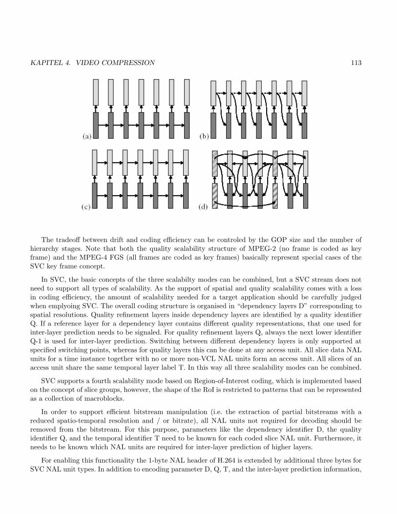
KAPITEL 4. VIDEO COMPRESSION 113
The tradeoff between drift and coding efficiency can be controled by the GOP size and the number ofhierarchy stages. Note that both the quality scalability structure of MPEG-2 (no frame is coded as keyframe) and the MPEG-4 FGS (all frames are coded as key frames) basically represent special cases of theSVC key frame concept.
In SVC, the basic concepts of the three scalabilty modes can be combined, but a SVC stream does notneed to support all types of scalability. As the support of spatial and quality scalability comes with a lossin coding efficiency, the amount of scalability needed for a target application should be carefully judgedwhen emplyoing SVC. The overall coding structure is organised in “dependency layers D” corresponding tospatial resolutions. Quality refinement layers inside dependency layers are identified by a quality identifierQ. If a reference layer for a dependency layer contains different quality representations, that one used forinter-layer prediction needs to be signaled. For quality refinement layers Q, always the next lower identifierQ-1 is used for inter-layer prediction. Switching between different dependency layers is only supported atspecified switching points, whereas for quality layers this can be done at any access unit. All slice data NALunits for a time instance together with no or more non-VCL NAL units form an access unit. All slices of anaccess unit share the same temporal layer label T. In this way all three scalability modes can be combined.
SVC supports a fourth scalability mode based on Region-of-Interest coding, which is implemented basedon the concept of slice groups, however, the shape of the RoI is restricted to patterns that can be representedas a collection of macroblocks.
In order to support efficient bitstream manipulation (i.e. the extraction of partial bitstreams with areduced spatio-temporal resolution and / or bitrate), all NAL units not required for decoding should beremoved from the bitstream. For this purpose, parameters like the dependency identifier D, the qualityidentifier Q, and the temporal identifier T need to be known for each coded slice NAL unit. Furthermore, itneeds to be known which NAL units are required for inter-layer prediction of higher layers.
For enabling this functionality the 1-byte NAL header of H.264 is extended by additional three bytes forSVC NAL unit types. In addition to encoding parameter D, Q, T, and the inter-layer prediction information,
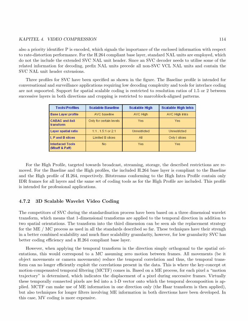
KAPITEL 4. VIDEO COMPRESSION 114
also a priority identifier P is encoded, which signals the importance of the enclosed information with respectto rate-distortion performance. For the H.264 compliant base layer, standard NAL units are employed, whichdo not the include the extended SVC NAL unit header. Since an SVC decoder needs to utilise some of therelated information for decoding, prefix NAL units precede all non-SVC VCL NAL units and contain theSVC NAL unit header extensions.
Three profiles for SVC have been specified as shown in the figure. The Baseline profile is intended forconversational and surveillance applications requiring low decoding complexity and tools for interlace codingare not supoorted. Support for spatial scalable coding is restricted to resolution ratios of 1.5 or 2 betweensuccessive layers in both directions and cropping is restricted to marcoblock-aligned patterns.
For the High Profile, targeted towards broadcast, streaming, storage, the described restrictions are re-moved. For the Baseline and the High profiles, the included H.264 base layer is compliant to the Baselineand the High profile of H.264, respectively. Bitstreams conforming to the High Intra Profile contain onlyIDR frames for all layers and the same set of coding tools as for the High Profile are included. This profileis intended for professional applications.
4.7.2 3D Scalable Wavelet Video Coding
The competitors of SVC during the standardisation process have been based on a three dimensioal wavelettransform, which means that 1-dimensional transforms are applied to the temporal direction in addition totwo spatial orientations. The transform into the third dimension can be seen als the replacement strategyfor the ME / MC process as used in all the standards described so far. These techniques have their strenghin a better combined scalability and much finer scalability granularity, however, for low granularity SVC hasbetter coding efficiency and a H.264 compliant base layer.
However, when applying the temporal transform in the direction simply orthogonal to the spatial ori-entations, this would correspond to a MC assuming zero motion between frames. All movements (be itobject movements or camera movements) reduce the temporal correlation and thus, the temporal trans-form can no longer efficiently exploit the correlations present in the data. This is where the key-concept otmotion-compensated temporal filtering (MCTF) comes in. Based on a ME process, for each pixel a “motiontrajectory” is determined, which indicates the displacement of a pixel during successive frames. Virtuallythese temporally connected pixels are fed into a 1-D vector onto which the temporal decomposition is ap-plied. MCTF can make use of ME information in one direction only (the Haar transform is then applied),but also techniques for longer filters involving ME information in both directions have been developed. Inthis case, MV coding is more expensive.

KAPITEL 4. VIDEO COMPRESSION 115
Of course, some problems arise related to “unconnected pixels” which are due to occlusions or suddenlyappearing objects. Motion compensated prediction is used locally to “filll the gaps” arising from this phe-nonemon. There are two basic architectures supporting this idea which are differentiated depending on inwhich stage of the process ME and the temporal decomposition is conducted. In t+2D schemes, ME is ap-plied in the spatial domain followed by the MCTF process. Subsequently, the resulting temporal frames aredecomposed in a 2-D wavelet transform for further decorrelation. In this approach it is very easy to integrate2-D wavelet coding schemes since these can be directly applied to the temporal frames (e.g. JPEG2000 andother scalable schemes can be applied here).
The second approach 2D+t is based on first applying a spatial 2-D wavelet transform to the framesof the original video. Subsequently, ME is done in the wavelet domain and the temporal decomposition isapplied along motion tranjectories filled with wavelet transform coefficients. Both approaches have somedisadvantages: t+2D cannot support spatial scalability well, since the motions vectors derived from fullresolution are not optimal for the lower spatial resolution (this problem is tackled by using scaled MV forexample). On the other hand, 2D+t suffers from the fact the ME cannot be done easily in the waveletdomain due to the lack if shift invariance in decimated schemes. Therefore overcomplate representations

KAPITEL 4. VIDEO COMPRESSION 116
without downsampling need to the applied for the ME process. There have been proposals suggesting tocombine both schemes in an adaptive process based on the nature of the video content.
A further improvement has been done by incorporating multi-scale pyramids in coding schemes of thistype which are usually called “2D+t+2D” schemes. Here, spatially scaled versions of the video are used whilethe coding scheme uses inter-scale prediction (ISP) in order to exploit multi-scale representation redundancy.As it was the case before, two different architecures have been designed which can be differnetiated dependingon where the pyramidal residue information is generated, before or after the MCTF.
One of the solutions discussed in SVC standardisation is similar to the latter technique, however, theISP technique is slightly different due to an additional wavelet transform being conducted to the temporalframes before ISP.
An additional argument against this type of techniques during standardisation was the higher memoryrequirements compared to SVC which makes hardware implementations more cost intensive. Also, is wasfound to be questionable if the superiority in terms of flexibility with respect to scalability is actually neededin applications. As we have seen in JPEG2000 or MPEG-4, not all capabilities of standardised codecs are

KAPITEL 4. VIDEO COMPRESSION 117
actually application relevant.
4.8 Non-standard Video Coding
Many video coding algorithms have been developed which never made it into standardisation due to variousreasons, since standardisation is always a political issue involving major companies and their correspondinginterests also with respect to patent issues. Therefore, superior technology is only one argument duringstandardisation.
Besides the multitude of 2-D schemes with ME/MC based on block-based DCT, a similar scheme basedon 2D global wavelet transform has been developed by the BBC (the DIRAC codec) which is also availableas open source and does a reasonable well job. This is just to show that it is also possible in principle to useother transforms instead of the DCT with good results.
3D video coding schemes have been proposed applying a wide variety of techniques (Wavelet, Fractal,DCT) among which 3D fractal video coding is again interesting from a scientific point of view since here, 3Dblock self similarities are exploited and decoding is conducted on arbitrary 3D blocks by applying the storedtransformations. In all of these schemes, the high computational encoding complexity and high momoryrequirements make them unsuited for general purpose standardisation despite of sometimes excellent codingperformance.
4.8.1 Distributed Video Coding
All video coding schemes discussed so far are highly assymetric in terms of computational complexity sinceencoding is much more demanding (usually orders of magnitude) as compared to decoding. While this isno problem in common streaming and retrieval-based applications, more recent application contexts likesensor networks or mobile capturing devices exhibit weak capturing and encoding devices which makes

KAPITEL 4. VIDEO COMPRESSION 118
the algorithms available so far entirely unsuited for these environments. Distributed video coding aimsat distributing the computational load in different manner between encoder and decoder thus enablingschemes with lightweight encoding but heavy decoding. In the figure a scheme including network basedtranscoding is shown which results in lightweight encoding and decoding in mobile capturing and displaydevices.
The basic facts behind this recent technology are based on the Slepian-Wolf (lossless) and Wyner-Ziv(lossy) coding principles. The fundamental idea is that correlated source signals X and Y can be compressedindependently – in case they are jointly decoded based on side information derived from their correlationthe same rate distortion performance can be achieved as in case of joint encoding.
When talking about video coding, the correlated signals X and Y represent temporally correlated framesof a video. In classical video coding, they are jointly encoded using ME / MC to exploit the temporalcorrelation. In distributed video coding the main idea is to shift ME to the decoder side and using thegenerated motion information is the side information required for joint decoding.
The two classical architectures have been developed at Stanford and UC Berkeley, repspectively. Webriefly describe the former. So-called key frames are encoded using a conventional intra-frame encodingscheme which are passed to the decoder. The Wyner-Ziv frames (which are the ones where the distributedcoding principle is applied) are subject to (optional) DCT transform and quantisation. The coefficientsare fed into a Turbo encoder (efficient error correcting coding scheme) on a bitplane basis, the resultingdata is fed into a buffer. In the decoder, the Turbo decoder starts decoding the MSB of the coefficients.Based on the side information coming from the decoded key frames it can be determined after some morerequested bit layers from the buffer, what a good quality reconstruction will be (ME is done based on

KAPITEL 4. VIDEO COMPRESSION 119
the coefficients approximation coming from the Turbo decoder and the decoded key frames and the higherbitplayer information is taken from the found match in the key frames).
To enable a more effective ME in the decoder, it has been suggested to transfer also additional (robust)hash values from the encoder to the decoder. Hash values can be generated quickly and only generate asmall bitrate overhead. They can be used to aid ME since when hashing is also applied to the key frames,corresponding hash values between those sent by the encoder (generated from the Wyner-Ziv frames) andthose computed by the decoder indicate a possible match between key frame block and Wyner-Ziv block.
While the overall concept is appealing, it has to be stated that compression performance is far belowthat of classical MC-based schemes used in standardisation, however, clearly improving upon compressionperformance of purely intra-coding scheme. Therefore, for specific application scenarios this technology isan interesting alternative – significant research efforts are still going on in this area.

Kapitel 5
Audio Coding
120
Related Documents