Lecture Notes 2: Matrices - Courant Institute of …cfgranda/pages/OBDA_fall17/notes... · 2017-09-20 · Optimization-based data analysis Fall 2017 Lecture Notes 2: Matrices Matrices

Optimization-based data analysis Fall 2017

Lecture Notes 2: Matrices

Matrices are rectangular arrays of numbers, which are extremely useful for data analysis.They can be interpreted as vectors in a vector space, linear functions or sets of vectors.

1 Basic properties

1.1 Column and row space

A matrix can be used to represent a set of vectors stored as columns or rows. The spanof these vectors are called the column and row space of the matrix respectively.

Definition 1.1 (Column and row space). The column space col (A) of a matrix A is thespan of its columns. The row space row (A) is the span of its rows.

Interestingly, the row space and the column space of all matrices have the same dimension.We name this quantity the rank of the matrix.

Definition 1.2 (Rank). The rank of a matrix is the dimension of its column and of itsrow space.

Theorem 1.3 (Proof in Section 5.1). The rank is well defined. For any matrix A

dim (col (A)) = dim (row (A)) . (1)

If the dimension of the row and column space of an m× n matrix where m < n is equalto m then the the rows are all linearly independent. Similarly, if m > n and the rankis n then the columns are all linearly independent. In general, when the rank equalsmin {n,m} we say that the matrix is full rank.

Recall that the inner product between two matrices A,B ∈ Rm×n is given by the trace ofATB, and the norm induced by this inner product is the Frobenius norm. If the columnspaces of two matrices are orthogonal, then the matrices are also orthogonal.

Lemma 1.4. If the column spaces of any pair of matrices A,B ∈ Rm×n are orthogonalthen

〈A,B〉 = 0. (2)

Proof. We can write the inner product as a sum of products between the columns of A

1

and B, which are all zero under the assumption of the lemma

〈A,B〉 := tr(ATB

)(3)

=n∑

i=1

〈A:,i, B:,i〉 (4)

= 0. (5)

The following corollary follows immediately from Lemma 1.4 and the Pythagorean theo-rem.

Corollary 1.5. If the column spaces of any pair of matrices A,B ∈ Rm×n are orthogonal

||A+B||2F = ||A||2F + ||B||2F . (6)

1.2 Linear maps

A map is a transformation that assigns a vector to another vector, possible belonging toa different vector space. The transformation is linear if it maps any linear combinationof input vectors to the same linear combination of the corresponding outputs.

Definition 1.6 (Linear map). Given two vector spaces V and R associated to the samescalar field, a linear map f : V → R is a map from vectors in V to vectors in R such thatfor any scalar α and any vectors ~x1, ~x2 ∈ V

f (~x1 + ~x2) = f (~x1) + f (~x2) , (7)

f (α~x1) = α f (~x1) . (8)

Every complex or real matrix of dimensions m × n defines a map from the space of n-dimensional vectors to the space of m-dimensional vectors through an operation calledmatrix-vector product. We denote the ith row of a matrix A by Ai:, the jth column byA:j and the (i, j) entry by Aij.

Definition 1.7 (Matrix-vector product). The product of a matrix A ∈ Cm×n and a vector~x ∈ Cn is a vector A~x ∈ Cm, such that

(A~x) [i] =n∑

j=1

Aij~x [j] . (9)

For real matrices, each entry in the matrix-vector product is the dot product between arow of the matrix and the vector,

(A~x) [i] = 〈Ai:, ~x〉 . (10)

2

The matrix-vector product can also be interpreted in terms of the column of the matrix,

A~x =n∑

j=1

~x [j]A:j. (11)

A~x is a linear combination of the columns of A weighted by the entries in ~x.

Matrix-vector multiplication is clearly linear. Perhaps surprisingly, the converse is alsotrue: any linear map between Cn and Cm (or between Rn and Rm) can be represented bya matrix.

Theorem 1.8 (Equivalence between matrices and linear maps). For finite m,n everylinear map f : Cm → Cn can be uniquely represented by a matrix F ∈ Cm×n.

Proof. The matrix is

F :=[f (~e1) f (~e2) · · · f (~en)

], (12)

i.e., the columns of the matrix are the result of applying f to the standard basis. Indeed,for any vector ~x ∈ Cn

f (x) = f

(n∑

i=1

~x[i]~ei

)(13)

=n∑

i=1

~x[i]f (~ei) by (7) and (8) (14)

= F~x. (15)

The ith column of any matrix that represents the linear map must equal f (~ei) by (11),so the representation is unique.

When a matrix Cm×n is fat, i.e., n > m, we often say that it projects vectors onto alower dimensional space. Note that such projections are not the same as the orthogonalprojections we described in Lecture Notes 1. When a matrix is tall, i.e., m > n, we saythat it lifts vectors to a higher-dimensional space.

1.3 Adjoint

The adjoint of a linear map f from an inner-product space V and another inner productspace R maps elements of R back to V in a way that preserves their inner product withimages of f .

Definition 1.9 (Adjoint). Given two vector spaces V and R associated to the same scalarfield with inner products 〈·, ·〉V and 〈·, ·〉R respectively, the adjoint f ∗ : R → V of a linearmap f : V → R satisfies

〈f (~x) , ~y〉R = 〈~x, f ∗ (~y)〉V (16)

for all ~x ∈ V and ~y ∈ R.

3

In the case of finite-dimensional spaces, the adjoint corresponds to the conjugate Hermi-tian transpose of the matrix associated to the linear map.

Definition 1.10 (Conjugate transpose). The entries of the conjugate transpose A∗ ∈Cn×m of a matrix A ∈ Cm×n are of the form

(A∗)ij = Aji, 1 ≤ i ≤ n, 1 ≤ j ≤ m. (17)

If the entries of the matrix are all real, this is just the transpose of the matrix.

Lemma 1.11 (Equivalence between conjugate transpose and adjoint). For finite m,nthe adjoint f ∗ : Cn → Cm of a linear map f : Cm → Cn represented by a matrix Fcorresponds to the conjugate transpose of the matrix F ∗.

Proof. For any ~x ∈ Cn and ~y ∈ Cm,

〈f (~x) , ~y〉Cm =m∑i=1

f (~x)i ~yi (18)

=m∑i=1

~yi

n∑j=1

Fij~xj (19)

=n∑

j=1

~xj

m∑i=1

Fij~yi (20)

= 〈~x, F ∗~y〉Cn . (21)

By Theorem 1.8 a linear map is represented by a unique matrix (you can check that theadjoint map is linear), which completes the proof.

A matrix that is equal to its adjoint is called self-adjoint. Self-adjoint real matricesare symmetric: they are equal to their transpose. Self-adjoint complex matrices areHermitian: they are equal to their conjugate transpose.

1.4 Range and null space

The range of a linear map is the set of all possible vectors that can be reached by applyingthe map.

Definition 1.12 (Range). Let V and R be vector spaces associated to the same scalarfield, the range of a map f : V → R is the set of vectors in R that can be reached byapplying f to a vector in V:

range (f) := {~y | ~y = f (~x) for some ~x ∈ V} . (22)

The range of a matrix is the range of its associated linear map.

4

The range of a matrix is the same as its column space.

Lemma 1.13 (The range is the column space). For any matrix A ∈ Cm×n

range (A) = col (A) . (23)

Proof. For any ~x, A~x is a linear combination of the columns of A, so the range is a subsetof the column space. In addition, every column of A is in the range, since A:i = A~ei for1 ≤ i ≤ n, so the column space is a subset of the range and both sets are equal.

The null space of a map is the set of vectors that are mapped to zero.

Definition 1.14 (Null space). Let V and R be vector spaces associated to the same scalarfield, the null space of a map f : V → R is the set of vectors in V that are mapped to thezero vector in R by f :

null (f) :={~x | f (~x) = ~0

}. (24)

The null space of a matrix is the null space of its associated linear map.

It is not difficult to prove that the null space of a map is a vector space, as long as themap is linear, since in that case scaling or adding elements of the null space yield vectorsthat are mapped to zero by the map.

The following lemma shows that for real matrices the null space is the orthogonal com-plement of the row space of the matrix.

Lemma 1.15. For any matrix A ∈ Rm×n

null (A) = row (A)⊥ . (25)

Proof. Any vector ~x in the row space of A can be written as ~x = AT~z, for some vector~z ∈ Rm. If y ∈ null (A) then

〈~y, ~x〉 =⟨~y, AT~z

⟩(26)

= 〈A~y, ~z〉 (27)

= 0. (28)

So null (A) ⊆ row (A)⊥.

If x ∈ row (A)⊥ then in particular it is orthogonal to every row of A, so Ax = 0 androw (A)⊥ ⊆ null (A).

An immediate corollary of Lemmas 1.13 and 1.15 is that the dimension of the range andthe null space add up to the ambient dimension of the row space.

Corollary 1.16. Let A ∈ Rm×n

dim (range (A)) + dim (null (A)) = n. (29)

This means that for every matrix A ∈ Rm×n we can decompose any vector in Rn into twocomponents: one is in the row space and is mapped to a nonzero vector in Cm, the otheris in the null space and is mapped to the zero vector.

5

1.5 Identity matrix and inverse

The identity matrix is a matrix that maps any vector to itself.

Definition 1.17 (Identity matrix). The identity matrix of dimensions n× n is

I =

1 0 · · · 00 1 · · · 0

· · ·0 0 · · · 1

. (30)

For any ~x ∈ Cn, I~x = ~x.

Square matrices have a unique inverse if they are full rank, since in that case the nullspace has dimension 0 and the associated linear map is a bijection. The inverse is a matrixthat reverses the effect of the matrix on any vector.

Definition 1.18 (Matrix inverse). The inverse of a square matrix A ∈ Cn×n is a matrixA−1 ∈ Cn×n such that

AA−1 = A−1A = I. (31)

1.6 Orthogonal and projection matrices

We often use the letters U ∈ Rm×n or V ∈ Rm×n for matrices with orthonormal columns.If such matrices are square then they are said to be orthogonal. Orthogonal matricesrepresent linear maps that do not affect the magnitude of a vector, just its direction.

Definition 1.19 (Orthogonal matrix). An orthogonal matrix is a real-valued square ma-trix such that its inverse is equal to its transpose,

UTU = UUT = I. (32)

By definition, the columns U:1, U:2, . . . , U:n of any n×n orthogonal matrix have unit normand orthogonal to each other, so they form an orthonormal basis (it’s somewhat confusingthat orthogonal matrices are not called orthonormal matrices instead). Applying UT to avector ~x ∈ Rn is equivalent to computing the coefficients of its representation in the basisformed by the columns of U . Applying U to UT~x recovers ~x by scaling each basis vectorwith the corresponding coefficient:

~x = UUT~x =n∑

i=1

〈U:i, ~x〉U:i. (33)

Since orthogonal matrices only rotate vectors, it is quite intuitive that the product of twoorthogonal matrices yields another orthogonal matrix.

6

Lemma 1.20 (Product of orthogonal matrices). If U, V ∈ Rn×n are orthogonal matrices,then UV is also an orthogonal matrix.

Proof.

(UV )T (UV ) = V TUTUV = I. (34)

The following lemma proves that orthogonal matrices preserve the `2 norms of vectors.

Lemma 1.21. Let U ∈ Rn×n be an orthogonal matrix. For any vector ~x ∈ Rn,

||U~x||2 = ||~x||2 . (35)

Proof. By the definition of orthogonal matrix

||U~x||22 = ~xTUTU~x (36)

= ~xT~x (37)

= ||~x||22 . (38)

Matrices with orthonormal columns can also be used to construct orthogonal-projectionmatrices, which represent orthogonal projections onto a subspace.

Lemma 1.22 (Orthogonal-projection matrix). Given a subspace S ⊆ Rn of dimensiond, the matrix

P := UUT , (39)

where the columns of U:1, U:2, . . . , U:d are an orthonormal basis of S, maps any vector ~xto its orthogonal projection onto S.

Proof. For any vector ~x ∈ Rn

P~x = UUT~x (40)

=d∑

i=1

〈U:i, ~x〉U:i (41)

= PS ~x by (64) in the lecture notes on vector spaces. (42)

2 Singular-value decomposition

In this section we introduce the singular-value decomposition, a fundamental tool formanipulating matrices, and describe several applications in data analysis.

7

2.1 Definition

Every real matrix has a singular-value decomposition.

Theorem 2.1. Every rank r real matrix A ∈ Rm×n, has a singular-value decomposition(SVD) of the form

A =[~u1 ~u2 · · · ~ur

]σ1 0 · · · 00 σ2 · · · 0

. . .

0 0 · · · σr

~v T1

~vT2...~vTr

(43)

= USV T , (44)

where the singular values σ1 ≥ σ2 ≥ · · · ≥ σr are positive real numbers, the left singularvectors ~u1, ~u2, . . .~ur form an orthonormal set, and the right singular vectors ~v1, ~v2, . . .~vralso form an orthonormal set. The SVD is unique if all the singular values are different.If several singular values are the same, their left singular vectors can be replaced by anyorthonormal basis of their span, and the same holds for the right singular vectors.

The SVD of an m× n matrix with m ≥ n can be computed in O (mn2). We refer to anygraduate linear algebra book for the proof of Theorem 2.1 and for the details on how tocompute the SVD.

The SVD provides orthonormal bases for the column and row spaces of the matrix.

Lemma 2.2. The left singular vectors are an orthonormal basis for the column space,whereas the right singular vectors are an orthonormal basis for the row space.

Proof. We prove the statement for the column space, the proof for the row space isidentical. All left singular vectors belong to the column space because ~ui = A

(σ−1i ~vi

). In

addition, every column of A is in their span because A:i = U(SV T~ei

). Since they form

an orthonormal set by Theorem 2.1, this completes the proof.

The SVD presented in Theorem 2.1 can be augmented so that the number of singularvalues equals min (m,n). The additional singular values are all equal to zero. Their cor-responding left and right singular vectors are orthonormal sets of vectors in the orthogonalcomplements of the column and row space respectively. If the matrix is tall or square,the additional right singular vectors are a basis of the null space of the matrix.

Corollary 2.3 (Singular-value decomposition). Every rank r real matrix A ∈ Rm×n,

8

where m ≥ n, has a singular-value decomposition (SVD) of the form

A := [ ~u1 ~u2 · · · ~ur︸ ︷︷ ︸Basis of range(A)

~ur+1 · · · ~un]

σ1 0 · · · 0 0 · · · 00 σ2 · · · 0 0 · · · 0

· · ·0 0 · · · σr 0 · · · 00 0 · · · 0 0 · · · 0

· · ·0 0 · · · 0 0 · · · 0

[~v1 ~v2 · · · ~vr︸ ︷︷ ︸Basis of row(A)

~vr+1 · · · ~vn︸ ︷︷ ︸Basis of null(A)

]T ,

(45)

where the singular values σ1 ≥ σ2 ≥ · · · ≥ σr are positive real numbers, the left singularvectors ~u1, ~u2, . . . , ~um form an orthonormal set in Rm, and the right singular vectors ~v1,~v2, . . . , ~vm form an orthonormal basis for Rn.

If the matrix is fat, we can define a similar augmentation, where the additional left singularvectors form an orthonormal basis of the orthogonal complement of the range.

By the definition of rank and Lemma 2.2 the rank of a matrix is equal to the number ofnonzero singular values.

Corollary 2.4. The rank of a matrix is equal to the number of nonzero singular values.

This interpretation of the rank allows to define an alternative definition that is very usefulin practice, since matrices are often full rank due to numerical error, even if their columnsor rows are almost linearly dependent.

Definition 2.5 (Numerical rank). Given a tolerance ε > 0, the numerical rank of a matrixis the number of singular values that are greater than ε.

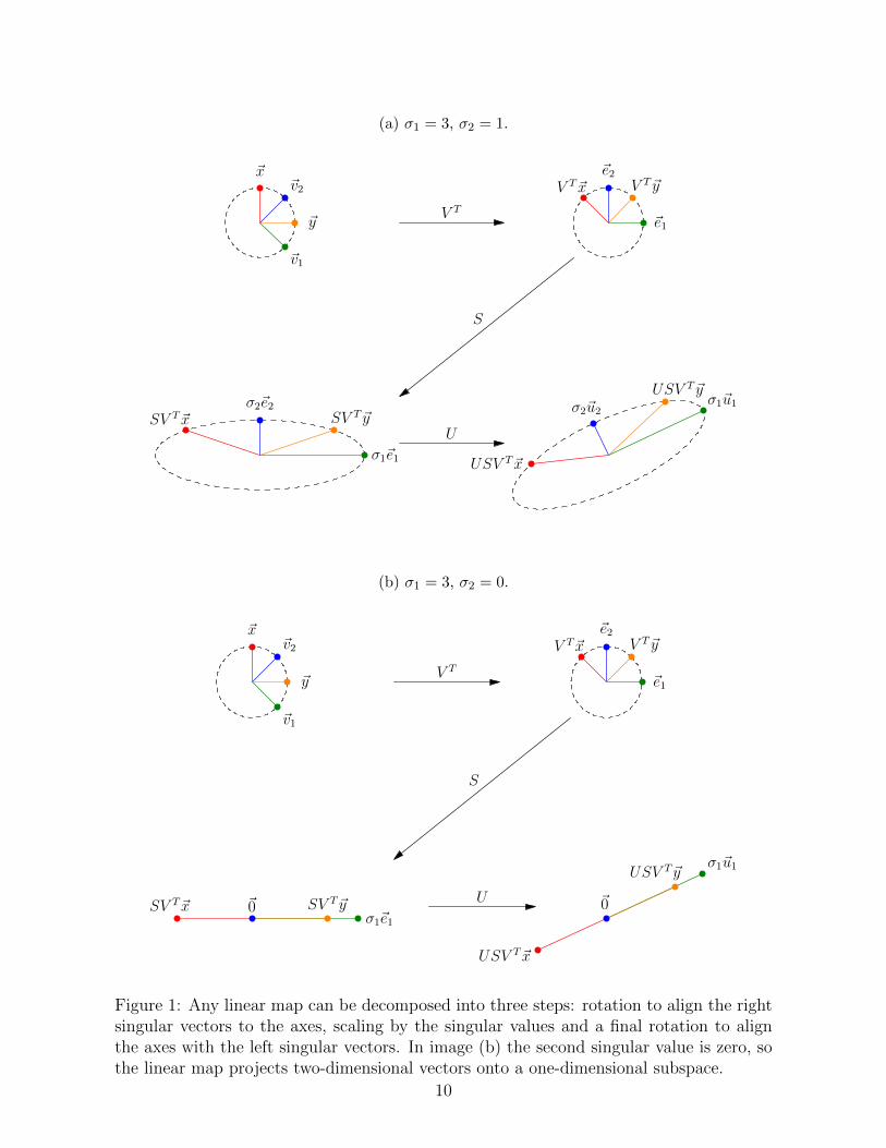
The SVD decomposes the action of a matrix A ∈ Rm×n on a vector ~x ∈ Rn into threesimple steps:

1. Rotation of ~x to align the component of ~x in the direction of the ith right singularvector ~vi with the ith axis:

V T~x =n∑

i=1

〈~vi, ~x〉~ei. (46)

2. Scaling of each axis by the corresponding singular value

SV T~x =n∑

i=1

σi 〈~vi, ~x〉~ei. (47)

3. Rotation to align the ith axis with the ith left singular vector

USV T~x =n∑

i=1

σi 〈~vi, ~x〉 ~ui. (48)

9

(a) σ1 = 3, σ2 = 1.

~x

~v1

~v2

~y

V T~x

~e1

~e2V T~y

SV T~x

σ1~e1

σ2~e2SV T~y

USV T~x

σ1~u1σ2~u2

USV T~y

V T

S

U

(b) σ1 = 3, σ2 = 0.

~x

~v1

~v2

~y

V T~x

~e1

~e2V T~y

SV T~xσ1~e1

~0 SV T~y

USV T~x

σ1~u1

~0

USV T~y

V T

S

U

Figure 1: Any linear map can be decomposed into three steps: rotation to align the rightsingular vectors to the axes, scaling by the singular values and a final rotation to alignthe axes with the left singular vectors. In image (b) the second singular value is zero, sothe linear map projects two-dimensional vectors onto a one-dimensional subspace.

10

Figure 1 illustrates this geometric analysis of the action of a linear map.

We end the section by showing that multiplying a matrix by an orthogonal matrix doesnot affect its singular values. This makes sense since it just modifies the rotation carriedout by the left or right singular vectors.

Lemma 2.6. For any matrix A ∈ Rm×n and any orthogonal matrices U ∈ Rm×m andV ∈ Rm×m the singular values of UA and AV are the same as the singular values of A.

Proof. Let A = USV T be the SVD of A. By Lemma 1.20 the matrices U := UU and

VT

:= V T V are orthogonal matrices, so USV T and USVT

are valid SVDs for UA andAV respectively. The result follows by unicity of the SVD.

2.2 Optimal approximations via the SVD

In the previous section, we show that linear maps rotate vectors, scale them according tothe singular values and then rotate them again. This means that the maximum scalingpossible is equal to the maximum singular value and occurs in the direction of the rightsingular vector ~v1. The following theorem makes this precise, showing that if we restrictour attention to the orthogonal complement of ~v1, then the maximum scaling is the secondsingular value, due to the orthogonality of the singular vectors. In general, the directionof maximum scaling orthogonal to the first i − 1 left singular vectors is equal to the ithsingular value and occurs in the direction of the ith singular vector.

Theorem 2.7. For any matrix A ∈ Rm×n, with SVD given by (45), the singular valuessatisfy

σ1 = max{||~x||2=1 | ~x∈Rn}

||A~x||2 (49)

= max{||~y||2=1 | ~y∈Rm}

∣∣∣∣AT~y∣∣∣∣

2, (50)

σi = max{||~x||2=1 | ~x∈Rn, ~x⊥~v1,...,~vi−1}

||A~x||2 , (51)

= max{||~y||2=1 | ~y∈Rm, ~y⊥~u1,...,~ui−1}

∣∣∣∣AT~y∣∣∣∣2, 2 ≤ i ≤ min {m,n} , (52)

the right singular vectors satisfy

~v1 = arg max{||~x||2=1 | ~x∈Rn}

||A~x||2 , (53)

~vi = arg max{||~x||2=1 | ~x∈Rn, ~x⊥~v1,...,~vi−1}

||A~x||2 , 2 ≤ i ≤ m, (54)

11

and the left singular vectors satisfy

~u1 = arg max{||~y||2=1 | ~y∈Rm}

∣∣∣∣AT~y∣∣∣∣2, (55)

~ui = arg max{||~y||2=1 | ~y∈Rm, ~y⊥~u1,...,~ui−1}

∣∣∣∣AT~y∣∣∣∣2, 2 ≤ i ≤ n. (56)

Proof. Consider a vector ~x ∈ Rn with unit `2 norm that is orthogonal to ~v1, . . . , ~vi−1,where 1 ≤ i ≤ n (if i = 1 then ~x is just an arbitrary vector). We express ~x in terms ofthe right singular vectors of A and a component that is orthogonal to their span

~x =n∑

j=i

αj~vj + Prow(A)⊥ ~x (57)

where 1 = ||~x||22 ≥∑n

j=i α2j . By the ordering of the singular values in Theorem 2.1

||A~x||22 =

⟨n∑

k=1

σk 〈~vk, ~x〉 ~uk,n∑

k=1

σk 〈~vk, ~x〉 ~uk

⟩by (48) (58)

=n∑

k=1

σ2k 〈~vk, ~x〉

2 because ~u1, . . . , ~un are orthonormal (59)

=n∑

k=1

σ2k

⟨~vk,

n∑j=i

αj~vj + Prow(A)⊥ ~x

⟩2

(60)

=n∑

j=i

σ2jα

2j because ~v1, . . . , ~vn are orthonormal (61)

≤ σ2i

n∑j=i

α2j because σi ≥ σi+1 ≥ . . . ≥ σn (62)

≤ σ2i by (57). (63)

This establishes (49) and (51). To prove (53) and (54) we show that ~vi achieves themaximum

||A~vi||22 =n∑

k=1

σ2k 〈~vk, ~vi〉

2 (64)

= σ2i . (65)

The same argument applied to AT establishes (50), (55), (56) and (52).

Given a set of vectors, it is often of interest to determine whether they are oriented inparticular directions of the ambient space. This can be quantified in terms of the `2norms of their projections on low-dimensional subspaces. The SVD provides an optimalk-dimensional subspace in this sense for any value of k.

12

Theorem 2.8 (Optimal subspace for orthogonal projection). For any matrix

A :=[~a1 ~a2 · · · ~an

]∈ Rm×n, (66)

with SVD given by (45), we have

n∑i=1

∣∣∣∣Pspan(~u1,~u2,...,~uk)~ai∣∣∣∣22≥

n∑i=1

||PS ~ai||22 , (67)

for any subspace S of dimension k ≤ min {m,n}.

Proof. Note that

n∑i=1

∣∣∣∣Pspan(~u1,~u2,...,~uk)~ai∣∣∣∣22

=n∑

i=1

k∑j=1

〈~uj,~ai〉2 (68)

=k∑

j=1

∣∣∣∣AT~uj∣∣∣∣22. (69)

We prove the result by induction on k. The base case k = 1 follows immediately from (55).To complete the proof we show that if the result is true for k − 1 ≥ 1 (the inductionhypothesis) then it also holds for k. Let S be an arbitrary subspace of dimension k. Theintersection of S and the orthogonal complement to the span of ~u1, ~u2,. . . , ~uk−1 containsa nonzero vector ~b due to the following lemma.

Lemma 2.9 (Proof in Section 5.2). In a vector space of dimension n, the intersectionof two subspaces with dimensions d1 and d2 such that d1 + d2 > n has dimension at leastone.

We choose an orthonormal basis ~b1,~b2, . . . ,~bk for S such that ~bk := ~b is orthogonal to~u1, ~u2, . . . , ~uk−1 (we can construct such a basis by Gram-Schmidt, starting with ~b). Bythe induction hypothesis,

k−1∑i=1

∣∣∣∣AT~ui∣∣∣∣2

2=

n∑i=1

∣∣∣∣Pspan(~u1,~u2,...,~uk−1)~ai∣∣∣∣22

(70)

≥n∑

i=1

∣∣∣∣∣∣Pspan(~b1,~b2,...,~bk−1)~ai

∣∣∣∣∣∣22

(71)

=k−1∑i=1

∣∣∣∣∣∣AT~bi

∣∣∣∣∣∣22. (72)

By (56) ∣∣∣∣AT~uk∣∣∣∣22≥∣∣∣∣∣∣AT~bk

∣∣∣∣∣∣22. (73)

13

Combining (72) and (73) we conclude

n∑i=1

∣∣∣∣Pspan(~u1,~u2,...,~uk)~ai∣∣∣∣22

=k∑

i=1

∣∣∣∣AT~ui∣∣∣∣22

(74)

≥k∑

i=1

∣∣∣∣∣∣AT~bi

∣∣∣∣∣∣22

(75)

=n∑

i=1

||PS ~ai||22 . (76)

The SVD also allows to compute the optimal k-rank approximation to a matrix in Frobe-nius norm, for any value of k. For any matrix A, we denote by A1:i,1:j to denote the i× jsubmatrix formed by taking the entries that are both in the first i rows and the first jcolumns. Similarly, we denote by A:,i:j the matrix formed by columns i to j.

Theorem 2.10 (Best rank-k approximation). Let USV T be the SVD of a matrix A ∈Rm×n. The truncated SVD U:,1:kS1:k,1:kV

T:,1:k is the best rank-k approximation of A in the

sense that

U:,1:kS1:k,1:kVT:,1:k = arg min

{A | rank(A)=k}

∣∣∣∣∣∣A− A∣∣∣∣∣∣F. (77)

Proof. Let A be an arbitrary matrix in Rm×n with rank(A) = k, and let U ∈ Rm×k be a

matrix with orthonormal columns such that col(U) = col(A). By Theorem 2.8,∣∣∣∣U:,1:kUT:,1:kA

∣∣∣∣2F

=n∑

i=1

∣∣∣∣∣∣Pcol(U:,1:k)~ai

∣∣∣∣∣∣22

(78)

≥n∑

i=1

∣∣∣∣∣∣Pcol(U)~ai

∣∣∣∣∣∣22

(79)

=∣∣∣∣∣∣U UTA

∣∣∣∣∣∣2F. (80)

The column space of A − U UTA is orthogonal to the column space of A and U , so byCorollary 1.5 ∣∣∣∣∣∣A− A∣∣∣∣∣∣2

F=∣∣∣∣∣∣A− U UTA

∣∣∣∣∣∣2F

+∣∣∣∣∣∣A− U UTA

∣∣∣∣∣∣2F

(81)

≥∣∣∣∣∣∣A− U UTA

∣∣∣∣∣∣2F

(82)

= ||A||2F −∣∣∣∣∣∣U UTA

∣∣∣∣∣∣2F

also by Corollary 1.5 (83)

≥ ||A||2F −∣∣∣∣U:,1:kU

T:,1:kA

∣∣∣∣2F

by (80) (84)

=∣∣∣∣A− U:,1:kU

T:,1:kA

∣∣∣∣2F

again by Corollary 1.5. (85)

14

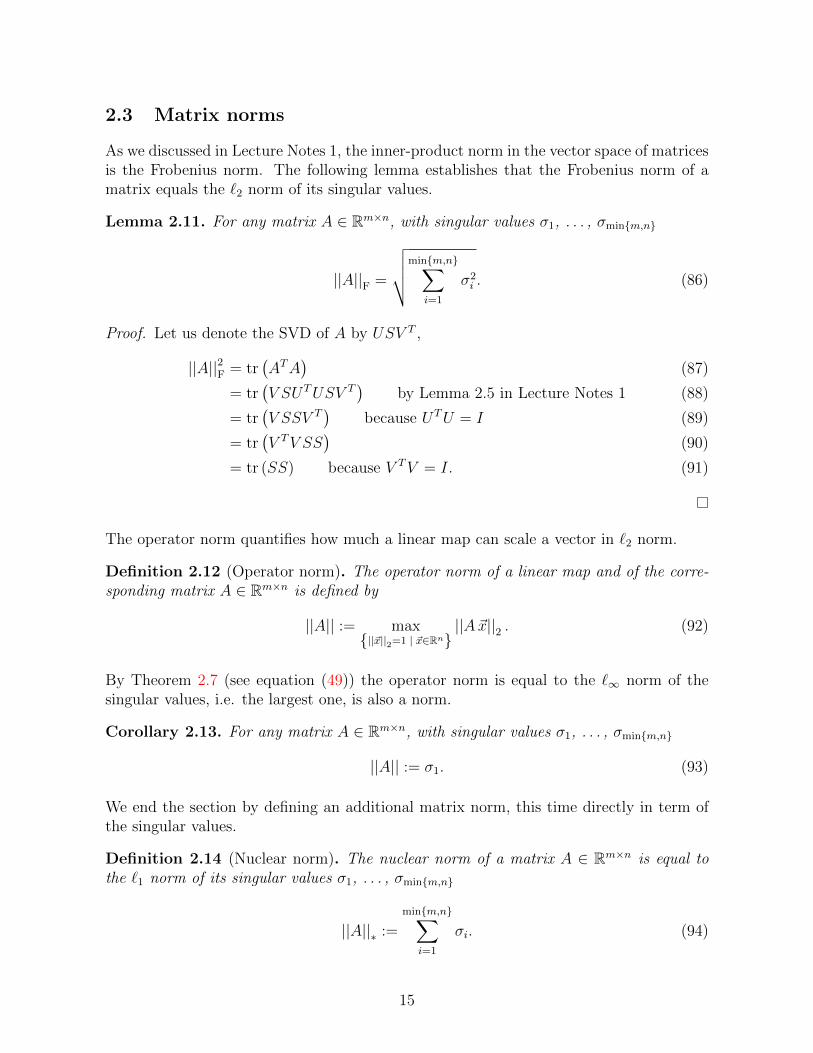
2.3 Matrix norms

As we discussed in Lecture Notes 1, the inner-product norm in the vector space of matricesis the Frobenius norm. The following lemma establishes that the Frobenius norm of amatrix equals the `2 norm of its singular values.

Lemma 2.11. For any matrix A ∈ Rm×n, with singular values σ1, . . . , σmin{m,n}

||A||F =

√√√√min{m,n}∑i=1

σ2i . (86)

Proof. Let us denote the SVD of A by USV T ,

||A||2F = tr(ATA

)(87)

= tr(V SUTUSV T

)by Lemma 2.5 in Lecture Notes 1 (88)

= tr(V SSV T

)because UTU = I (89)

= tr(V TV SS

)(90)

= tr (SS) because V TV = I. (91)

The operator norm quantifies how much a linear map can scale a vector in `2 norm.

Definition 2.12 (Operator norm). The operator norm of a linear map and of the corre-sponding matrix A ∈ Rm×n is defined by

||A|| := max{||~x||2=1 | ~x∈Rn}

||A~x||2 . (92)

By Theorem 2.7 (see equation (49)) the operator norm is equal to the `∞ norm of thesingular values, i.e. the largest one, is also a norm.

Corollary 2.13. For any matrix A ∈ Rm×n, with singular values σ1, . . . , σmin{m,n}

||A|| := σ1. (93)

We end the section by defining an additional matrix norm, this time directly in term ofthe singular values.

Definition 2.14 (Nuclear norm). The nuclear norm of a matrix A ∈ Rm×n is equal tothe `1 norm of its singular values σ1, . . . , σmin{m,n}

||A||∗ :=

min{m,n}∑i=1

σi. (94)

15

Any matrix norm that is a function of the singular values of a matrix is preserved aftermultiplication by an orthogonal matrix. This is a direct corollary of Lemma 2.6.

Corollary 2.15. For any matrix A ∈ Rm×n and any orthogonal matrices U ∈ Rm×m andV ∈ Rn×n the operator, Frobenius and nuclear norm of UA and AV are the same as thoseof A.

The following theorem is analogous to Holder’s inequality for vectors.

Theorem 2.16 (Proof in Section 5.3). For any matrix A ∈ Rm×n,

||A||∗ = sup{||B||≤1 | B∈Rm×n}

〈A,B〉 . (95)

A direct consequence of the result is that the nuclear norm satisfies the triangle inequality.This implies that it is a norm, since it clearly satisfies the remaining properties.

Corollary 2.17. For any m× n matrices A and B

||A+B||∗ ≤ ||A||∗ + ||B||∗ . (96)

Proof.

||A+B||∗ = sup{||C||≤1 | C∈Rm×n}

〈A+B,C〉 (97)

≤ sup{||C||≤1 | C∈Rm×n}

〈A,C〉+ sup{||D||≤1 | D∈Rm×n}

〈B,D〉 (98)

= ||A||∗ + ||B||∗ . (99)

2.4 Denoising via low-rank matrix estimation

In this section we consider the problem of denoising a set of n m-dimensional signals ~x1,~x2, . . . , ~xn ∈ Rm. We model the noisy data as the sum between each signal and a noisevector

~yi = ~xi + ~zi, 1 ≤ i ≤ n. (100)

Our first assumption is that the signals are similar, in the sense that they approximatelyspan a low-dimensional subspace due to the correlations between them. If this is the case,then the matrix

X :=[~x1 ~x2 · · · ~xn

](101)

obtained by stacking the signals as columns is approximately low rank. Note that incontrast to the subspace-projection denoising method described in Lecture Notes 1, wedo not assume that the subspace is known.

16

Our second assumption is that the noise vectors are independent from each other, so thatthe noise matrix

Z :=[~z1 ~z2 · · · ~zn

](102)

is full rank. If the noise is not too large with respect to the signals, under these assump-tions a low-rank approximation to the data matrix

Y :=[~y1 ~y2 · · · ~yn

](103)

= X + Z (104)

should mostly suppress the noise and extract the component corresponding to the signals.Theorem 2.10 establishes that the best rank-k approximation to a matrix in Frobeniusnorm is achieved by truncating the SVD, for any value of k.

Algorithm 2.18 (Denoising via SVD truncation). Given n noisy data vectors ~y1, ~y2, . . . , ~yn ∈Rm, we denoise the data by

1. Stacking the vectors as the columns of a matrix Y ∈ Rm×n.

2. Computing the SVD of Y = USV T .

3. Truncating the SVD to produce the low-rank estimate L

L := U:,1:kS1:k,1:kVT:,1:k, (105)

for a fixed value of k ≤ min {m,n}.

An important decision is what rank k to choose. Higher ranks yield more accurate approx-imations to the original signals than lower-rank approximations, but they do not suppressthe noise component in the data as much. The following example illustrates this tradeoff.

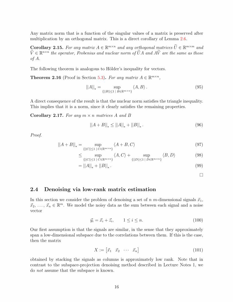
Example 2.19 (Denoising of digit images). In this example we use the MNIST data set1

to illustrate image denoising using SVD truncation. The signals consist of 6131 28 × 28images of the number 3. The images are corrupted by noise sampled independently froma Gaussian distribution and scaled so that the signal-to-noise ratio (defined as the ratiobetween the `2 norms of the clean image and the noise) is 0.5 (there is more noise thansignal!). Our assumption is that because of their similarities, the images interpretedas vectors in R784 form a low-dimensional (but unknown subspace), whereas the noiseis uncorrelated and therefore is not restricted to a subspace. This assumption holds:Figure 11 shows the singular values of matrix formed by stacking the clean images, thenoisy images and the noise.

We center each noisy image by subtracting the average of all the noisy images. Subtractingthe average is a common preprocessing step in low-rank approximations (see Figure 5 fora geometric justification). We then apply SVD truncation to obtain a low-rank estimateof the image matrix. The noisy average is then added back to the images to produce thefinal estimate of the images. Figure 3 shows the results for rank-10 and rank-40 estimates.The lower-rank estimate suppresses the noise more, but does not approximate the originalsignals as effectively. 41Available at http://yann.lecun.com/exdb/mnist/

17

0 10 20 30 40 500

500

1,000

1,500

i

σi

0 200 400 6000

500

1,000

1,500

i

σi

DataSignalsNoise

Figure 2: Plots of the singular values of the clean images, the noisy images and the noisein Example 2.19.

Signals

Rank 40approx.

Rank 10approx.

Rank 40est.

Rank 10est.

Data

Figure 3: The images show 9 examples from the 6131 images used in Example 2.19. Thetop row shows the original clean images. The second and third rows show rank-40 andrank-10 approximations to the clean images. The fourth and fifth rows shows the resultsof applying SVD truncation to obtain rank-40 and rank-10 estimates respectively. Thesixth row shows the noisy data.

18

2.5 Collaborative filtering

The aim of collaborative filtering is to pool together information from many users to obtaina model of their behavior. To illustrate the use of low-rank models in this application weconsider a toy example. Bob, Molly, Mary and Larry rate the following six movies from1 to 5,

A :=

Bob Molly Mary Larry

1 1 5 4 The Dark Knight2 1 4 5 Spiderman 34 5 2 1 Love Actually5 4 2 1 Bridget Jones’s Diary4 5 1 2 Pretty Woman1 2 5 5 Superman 2

(106)

A common assumption in collaborative filtering is that there are people that have similartastes and hence produce similar ratings, and that there are movies that are similar andhence elicit similar reactions. Interestingly, this tends to induce low-rank structure in thematrix of ratings. To uncover this low-rank structure, we first subtract the average rating

µ :=1

mn

m∑i=1

n∑j=1

Aij, (107)

from each entry in the matrix to obtain a centered matrix C and then compute its singular-value decomposition

A− µ~1~1T = USV T = U

7.79 0 0 0

0 1.62 0 00 0 1.55 00 0 0 0.62

V T . (108)

where ~1 ∈ R4 is a vector of ones. The fact that the first singular value is significantlylarger than the rest suggests that the matrix may be well approximated by a rank-1matrix. This is indeed the case:

µ~1~1T + σ1~u1~vT1 =

Bob Molly Mary Larry

1.34 (1) 1.19 (1) 4.66 (5) 4.81 (4) The Dark Knight1.55 (2) 1.42 (1) 4.45 (4) 4.58 (5) Spiderman 34.45 (4) 4.58 (5) 1.55 (2) 1.42 (1) Love Actually4.43 (5) 4.56 (4) 1.57 (2) 1.44 (1) Bridget Jones’s Diary4.43 (4) 4.56 (5) 1.57 (1) 1.44 (2) Pretty Woman1.34 (1) 1.19 (2) 4.66 (5) 4.81 (5) Superman 2

(109)

19

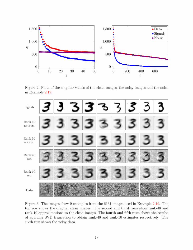
For ease of comparison the values of A are shown in brackets. The first left singular vectoris equal to

~u1 :=D. Knight Spiderman 3 Love Act. B.J.’s Diary P. Woman Superman 2

( )−0.45 −0.39 0.39 0.39 0.39 −0.45 .

This vector allows us to cluster the movies: movies with negative entries are similar (inthis case they correspond to action movies) and movies with positive entries are similar(in this case they are romantic movies).

The first right singular vector is equal to

~v1 =Bob Molly Mary Larry

( )0.48 0.52 −0.48 −0.52 . (110)

This vector allows to cluster the users: negative entries indicate users that like actionmovies but hate romantic movies (Bob and Molly), whereas positive entries indicate thecontrary (Mary and Larry).

For larger data sets, the model generalizes to a rank-k approximation, which approximateseach ranking by a sum of k terms

rating (movie i, user j) =k∑

l=1

σl~ul [i]~vl [j] . (111)

The singular vectors cluster users and movies in different ways, whereas the singular valuesweight the importance of the different factors.

3 Principal component analysis

In Lecture Notes 1 we introduced the sample variance of a set of one-dimensional data,which measures the variation of measurements in a one-dimensional data set, as well as thesample covariance, which measures the joint fluctuations of two features. We now considerdata sets where each example contains m features, and can therefore be interpreted as avector in an m-dimensional ambient space. We are interested in analyzing the variationof the data in different directions of this space.

3.1 Sample covariance matrix

The sample covariance matrix of a data set contains the pairwise sample covariance be-tween every pair of features in a data set. If the data are sampled from a multivariatedistribution, then the sample covariance matrix can be interpreted as an estimate of thecovariance matrix (see Section 3.3).

20

Definition 3.1 (Sample covariance matrix). Let {~x1, ~x2, . . . , ~xn} be a set of m-dimensionalreal-valued data vectors, where each dimension corresponds to a different feature. Thesample covariance matrix of these vectors is the m×m matrix

Σ (~x1, . . . , ~xn) :=1

n− 1

n∑i=1

(~xi − av (~x1, . . . , ~xn)) (~xi − av (~x1, . . . , ~xn))T , (112)

where the center or average is defined as

av (~x1, ~x2, . . . , ~xn) :=1

n

n∑i=1

~xi (113)

contains the sample mean of each feature. The (i, j) entry of the covariance matrix, where1 ≤ i, j ≤ d, is given by

Σ (~x1, . . . , ~xn)ij =

{var (~x1 [i] , . . . , ~xn [i]) if i = j,

cov ((~x1 [i] , ~x1 [j]) , . . . , (~xn [i] , ~xn [j])) if i 6= j.(114)

In order to characterize the variation of a multidimensional data set around its center,we consider its variation in different directions. The average variation of the data in acertain direction is quantified by the sample variance of the projections of the data ontothat direction. Let ~d ∈ Rm be a unit-norm vector aligned with a direction of interest, thesample variance of the data set in the direction of ~d is given by

var(~d T~x1, . . . , ~d

T~xn

)=

1

n− 1

n∑i=1

(~d T~xi − av

(~d T~x1, . . . , ~d

T~xn

))2(115)

=1

n− 1

n∑i=1

(~d T (~xi − av (~x1, . . . , ~xn))

)2(116)

= ~d T

(1

n− 1

n∑i=1

(~xi − av (~x1, . . . , ~xn)) (~xi − av (~x1, . . . , ~xn))T)~d

= ~d TΣ (~x1, . . . , ~xn) ~d. (117)

Using the sample covariance matrix we can express the variation in every direction! Thisis a deterministic analog of the fact that the covariance matrix of a random vector encodesits variance in every direction.

3.2 Principal component analysis

Principal-component analysis is a popular tool for data analysis, which consists of com-puting the singular-value decomposition of a set of vectors grouped as the columns of amatrix.

21

σ1/√n− 1 = 0.705,

σ2/√n− 1 = 0.690

σ1/√n− 1 = 0.983,

σ2/√n− 1 = 0.356

σ1/√n− 1 = 1.349,

σ2/√n− 1 = 0.144

~u1

~u2

v1

v2

~u1

~u2

~u1

~u2

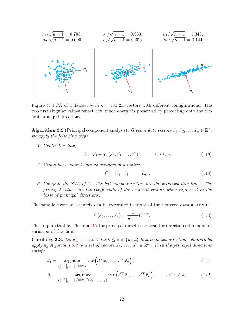
Figure 4: PCA of a dataset with n = 100 2D vectors with different configurations. Thetwo first singular values reflect how much energy is preserved by projecting onto the twofirst principal directions.

Algorithm 3.2 (Principal component analysis). Given n data vectors ~x1, ~x2, . . . , ~xn ∈ Rd,we apply the following steps.

1. Center the data,

~ci = ~xi − av (~x1, ~x2, . . . , ~xn) , 1 ≤ i ≤ n. (118)

2. Group the centered data as columns of a matrix

C =[~c1 ~c2 · · · ~cn

]. (119)

3. Compute the SVD of C. The left singular vectors are the principal directions. Theprincipal values are the coefficients of the centered vectors when expressed in thebasis of principal directions.

The sample covariance matrix can be expressed in terms of the centered data matrix C

Σ (~x1, . . . , ~xn) =1

n− 1CCT . (120)

This implies that by Theorem 2.7 the principal directions reveal the directions of maximumvariation of the data.

Corollary 3.3. Let ~u1, . . . , ~uk be the k ≤ min {m,n} first principal directions obtained byapplying Algorithm 3.2 to a set of vectors ~x1, . . . , ~xn ∈ Rm. Then the principal directionssatisfy

~u1 = arg max{||~d||

2=1 | ~d∈Rn}

var(~d T~x1, . . . , ~d

T~xn

), (121)

~ui = arg max{||~d||

2=1 | ~d∈Rn, ~d⊥~u1,...,~ui−1}

var(~d T~x1, . . . , ~d

T~xn

), 2 ≤ i ≤ k, (122)

22

σ1/√n− 1 = 5.077 σ1/

√n− 1 = 1.261

σ2/√n− 1 = 0.889 σ2/

√n− 1 = 0.139

~u1

~u2

~u2

~u1

Uncentered data Centered data

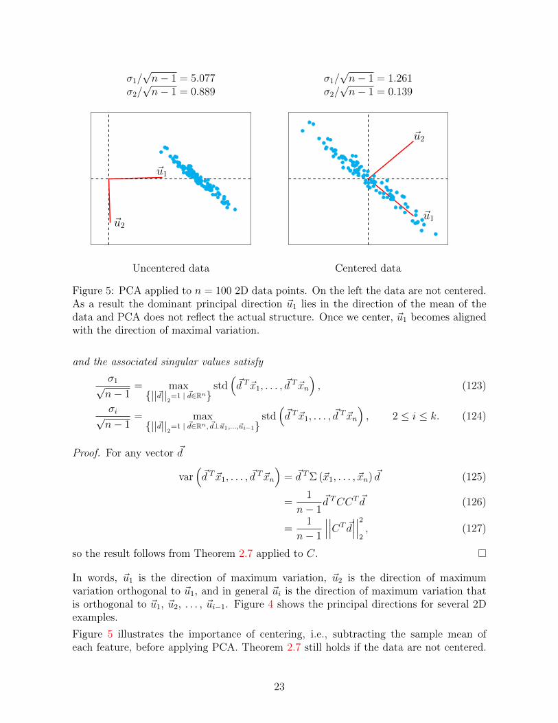
Figure 5: PCA applied to n = 100 2D data points. On the left the data are not centered.As a result the dominant principal direction ~u1 lies in the direction of the mean of thedata and PCA does not reflect the actual structure. Once we center, ~u1 becomes alignedwith the direction of maximal variation.

and the associated singular values satisfy

σ1√n− 1

= max{||~d||

2=1 | ~d∈Rn}

std(~d T~x1, . . . , ~d

T~xn

), (123)

σi√n− 1

= max{||~d||

2=1 | ~d∈Rn, ~d⊥~u1,...,~ui−1}

std(~d T~x1, . . . , ~d

T~xn

), 2 ≤ i ≤ k. (124)

Proof. For any vector ~d

var(~d T~x1, . . . , ~d

T~xn

)= ~d TΣ (~x1, . . . , ~xn) ~d (125)

=1

n− 1~d TCCT ~d (126)

=1

n− 1

∣∣∣∣∣∣CT ~d∣∣∣∣∣∣22, (127)

so the result follows from Theorem 2.7 applied to C.

In words, ~u1 is the direction of maximum variation, ~u2 is the direction of maximumvariation orthogonal to ~u1, and in general ~ui is the direction of maximum variation thatis orthogonal to ~u1, ~u2, . . . , ~ui−1. Figure 4 shows the principal directions for several 2Dexamples.

Figure 5 illustrates the importance of centering, i.e., subtracting the sample mean ofeach feature, before applying PCA. Theorem 2.7 still holds if the data are not centered.

23

Center PD 1 PD 2 PD 3 PD 4 PD 5

σi/√n− 1 330 251 192 152 130

PD 10 PD 15 PD 20 PD 30 PD 40 PD 50

90.2 70.8 58.7 45.1 36.0 30.8

PD 100 PD 150 PD 200 PD 250 PD 300 PD 359

19.0 13.7 10.3 8.01 6.14 3.06

Figure 6: Average and principal directions (PD) of the faces data set in Example 3.4,along with their associated singular values.

However, the norm of the projection onto a certain direction no longer reflects the variationof the data. In fact, if the data are concentrated around a point that is far from theorigin, the first principal direction tends be aligned with that point. This makes sense asprojecting onto that direction captures more energy. As a result, the principal directionsdo not reflect the directions of maximum variation within the cloud of data. Centeringthe data set before applying PCA solves the issue.

In the following example, we apply PCA to a set of images.

Example 3.4 (PCA of faces). In this example we consider the Olivetti Faces data set,which we described in Lecture Notes 1. We apply Algorithm 3.2 to a data set of 40064 × 64 images taken from 40 different subjects (10 per subject). We vectorize each im-age so that each pixel is interpreted as a different feature. Figure 6 shows the centerof the data and several principal directions, together with their associated singular val-ues. The principal directions corresponding to the larger singular values seem to capturelow-resolution structure, whereas the ones corresponding to the smallest singular valuesincorporate more intricate details.

24

Center PD 1 PD 2 PD 3

= 8613 - 2459 + 665 - 180

+ 301 + 566 + 638 + 403

PD 4 PD 5 PD 6 PD 7

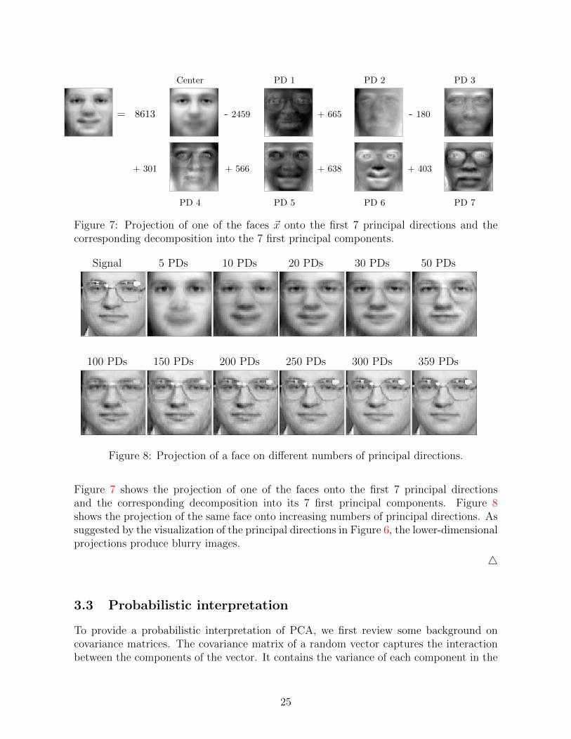
Figure 7: Projection of one of the faces ~x onto the first 7 principal directions and thecorresponding decomposition into the 7 first principal components.

Signal 5 PDs 10 PDs 20 PDs 30 PDs 50 PDs

100 PDs 150 PDs 200 PDs 250 PDs 300 PDs 359 PDs

Figure 8: Projection of a face on different numbers of principal directions.

Figure 7 shows the projection of one of the faces onto the first 7 principal directionsand the corresponding decomposition into its 7 first principal components. Figure 8shows the projection of the same face onto increasing numbers of principal directions. Assuggested by the visualization of the principal directions in Figure 6, the lower-dimensionalprojections produce blurry images.

4

3.3 Probabilistic interpretation

To provide a probabilistic interpretation of PCA, we first review some background oncovariance matrices. The covariance matrix of a random vector captures the interactionbetween the components of the vector. It contains the variance of each component in the

25

diagonal and the covariances between different components in the off diagonals.

Definition 3.5. The covariance matrix of a random vector ~x is defined as

Σ~x :=

Var (~x [1]) Cov (~x [1] , ~x [2]) · · · Cov (~x [1] , ~x [n])

Cov (~x [2] , ~x [1]) Var (~x [2]) · · · Cov (~x [2] , ~x [n])...

.... . .

...Cov (~x [n] , ~x [1]) Cov (~x [n] , ~x [2]) · · · Var (~x [n])

(128)

= E(~x~xT

)− E(~x)E(~x)T . (129)

Note that if all the entries of a vector are uncorrelated, then its covariance matrix isdiagonal. Using linearity of expectation, we obtain a simple expression for the covariancematrix of the linear transformation of a random vector.

Theorem 3.6 (Covariance matrix after a linear transformation). Let ~x be a randomvector of dimension n with covariance matrix Σ. For any matrix A ∈ Rm×n ,

ΣA~x = AΣ~xAT . (130)

Proof. By linearity of expectation

ΣA~x = E(

(A~x) (A~x)T)− E (A~x) E (A~x)T (131)

= A(E(~x~xT

)− E(~x)E(~x)T

)AT (132)

= AΣ~xAT . (133)

An immediate corollary of this result is that we can easily decode the variance of therandom vector in any direction from the covariance matrix. Mathematically, the varianceof the random vector in the direction of a unit vector ~v is equal to the variance of itsprojection onto ~v.

Corollary 3.7. Let ~v be a unit-`2-norm vector,

Var(~v T~x

)= ~v TΣ~x~v. (134)

Consider the SVD of the covariance matrix of an n-dimensional random vector X

Σ~x = UΛUT (135)

=[~u1 ~u2 · · · ~un

] σ1 0 · · · 00 σ2 · · · 0

· · ·0 0 · · · σn

[~u1 ~u2 · · · ~un]T. (136)

Covariance matrices are symmetric by definition, so by Theorem 4.3 the eigenvectors ~u1,~u2, . . . , ~un can be chosen to be orthogonal. These singular vectors and singular valuescompletely characterize the variance of the random vector in different directions. Thetheorem is a direct consequence of Corollary 3.7 and Theorem 2.7.

26

√σ1 = 1.22,

√σ2 = 0.71

√σ1 = 1,

√σ2 = 1

√σ1 = 1.38,

√σ2 = 0.32

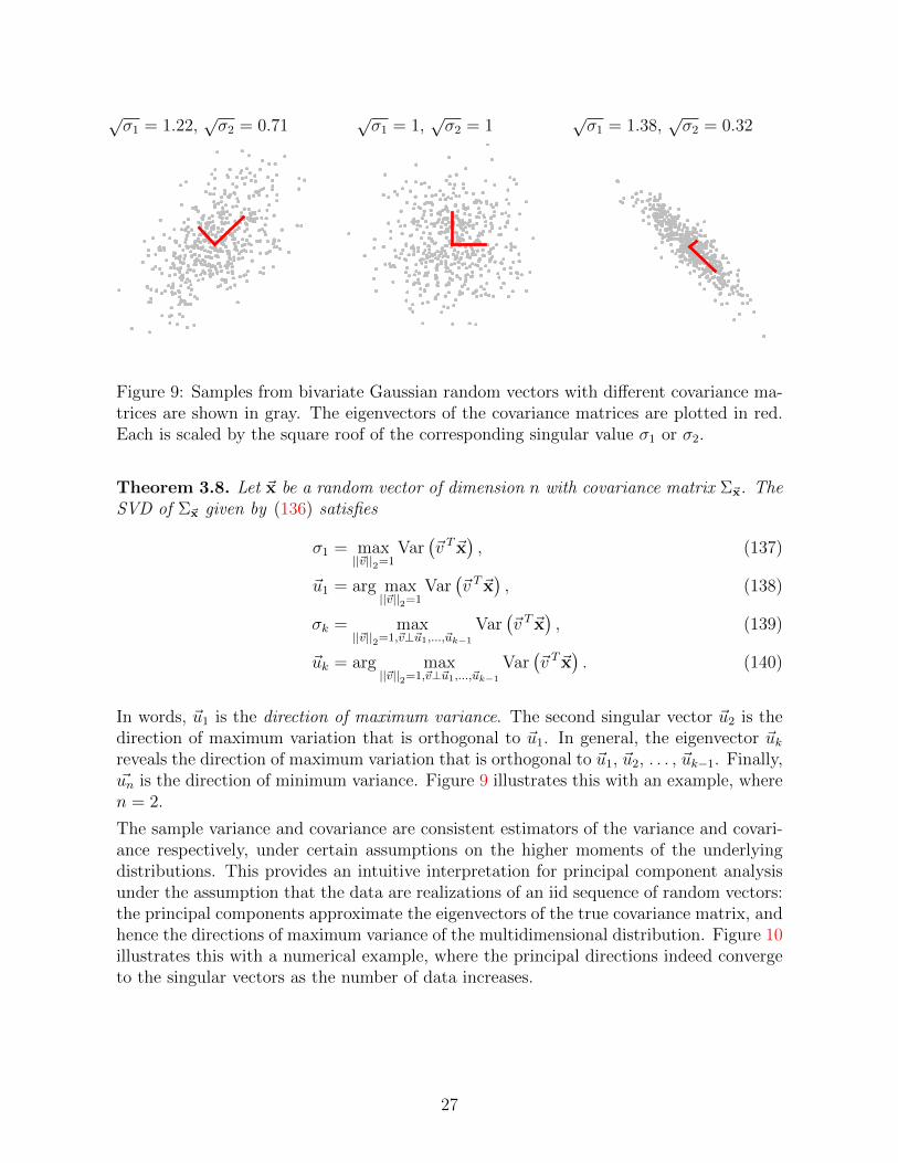
Figure 9: Samples from bivariate Gaussian random vectors with different covariance ma-trices are shown in gray. The eigenvectors of the covariance matrices are plotted in red.Each is scaled by the square roof of the corresponding singular value σ1 or σ2.

Theorem 3.8. Let ~x be a random vector of dimension n with covariance matrix Σ~x. TheSVD of Σ~x given by (136) satisfies

σ1 = max||~v||2=1

Var(~v T~x

), (137)

~u1 = arg max||~v||2=1

Var(~v T~x

), (138)

σk = max||~v||2=1,~v⊥~u1,...,~uk−1

Var(~v T~x

), (139)

~uk = arg max||~v||2=1,~v⊥~u1,...,~uk−1

Var(~v T~x

). (140)

In words, ~u1 is the direction of maximum variance. The second singular vector ~u2 is thedirection of maximum variation that is orthogonal to ~u1. In general, the eigenvector ~ukreveals the direction of maximum variation that is orthogonal to ~u1, ~u2, . . . , ~uk−1. Finally,~un is the direction of minimum variance. Figure 9 illustrates this with an example, wheren = 2.

The sample variance and covariance are consistent estimators of the variance and covari-ance respectively, under certain assumptions on the higher moments of the underlyingdistributions. This provides an intuitive interpretation for principal component analysisunder the assumption that the data are realizations of an iid sequence of random vectors:the principal components approximate the eigenvectors of the true covariance matrix, andhence the directions of maximum variance of the multidimensional distribution. Figure 10illustrates this with a numerical example, where the principal directions indeed convergeto the singular vectors as the number of data increases.

27

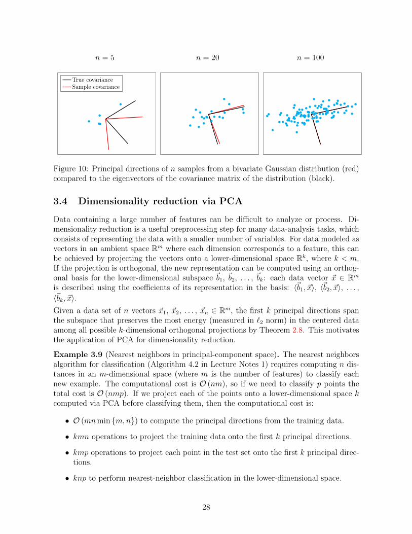
n = 5 n = 20 n = 100

True covarianceSample covariance

Figure 10: Principal directions of n samples from a bivariate Gaussian distribution (red)compared to the eigenvectors of the covariance matrix of the distribution (black).

3.4 Dimensionality reduction via PCA

Data containing a large number of features can be difficult to analyze or process. Di-mensionality reduction is a useful preprocessing step for many data-analysis tasks, whichconsists of representing the data with a smaller number of variables. For data modeled asvectors in an ambient space Rm where each dimension corresponds to a feature, this canbe achieved by projecting the vectors onto a lower-dimensional space Rk, where k < m.If the projection is orthogonal, the new representation can be computed using an orthog-onal basis for the lower-dimensional subspace ~b1, ~b2, . . . , ~bk: each data vector ~x ∈ Rm

is described using the coefficients of its representation in the basis: 〈~b1, ~x〉, 〈~b2, ~x〉, . . . ,

〈~bk, ~x〉.Given a data set of n vectors ~x1, ~x2, . . . , ~xn ∈ Rm, the first k principal directions spanthe subspace that preserves the most energy (measured in `2 norm) in the centered dataamong all possible k-dimensional orthogonal projections by Theorem 2.8. This motivatesthe application of PCA for dimensionality reduction.

Example 3.9 (Nearest neighbors in principal-component space). The nearest neighborsalgorithm for classification (Algorithm 4.2 in Lecture Notes 1) requires computing n dis-tances in an m-dimensional space (where m is the number of features) to classify eachnew example. The computational cost is O (nm), so if we need to classify p points thetotal cost is O (nmp). If we project each of the points onto a lower-dimensional space kcomputed via PCA before classifying them, then the computational cost is:

• O (mnmin {m,n}) to compute the principal directions from the training data.

• kmn operations to project the training data onto the first k principal directions.

• kmp operations to project each point in the test set onto the first k principal direc-tions.

• knp to perform nearest-neighbor classification in the lower-dimensional space.

28

0 10 20 30 40 50 60 70 80 90 100

10

20

30

4

Number of principal components

Err

ors

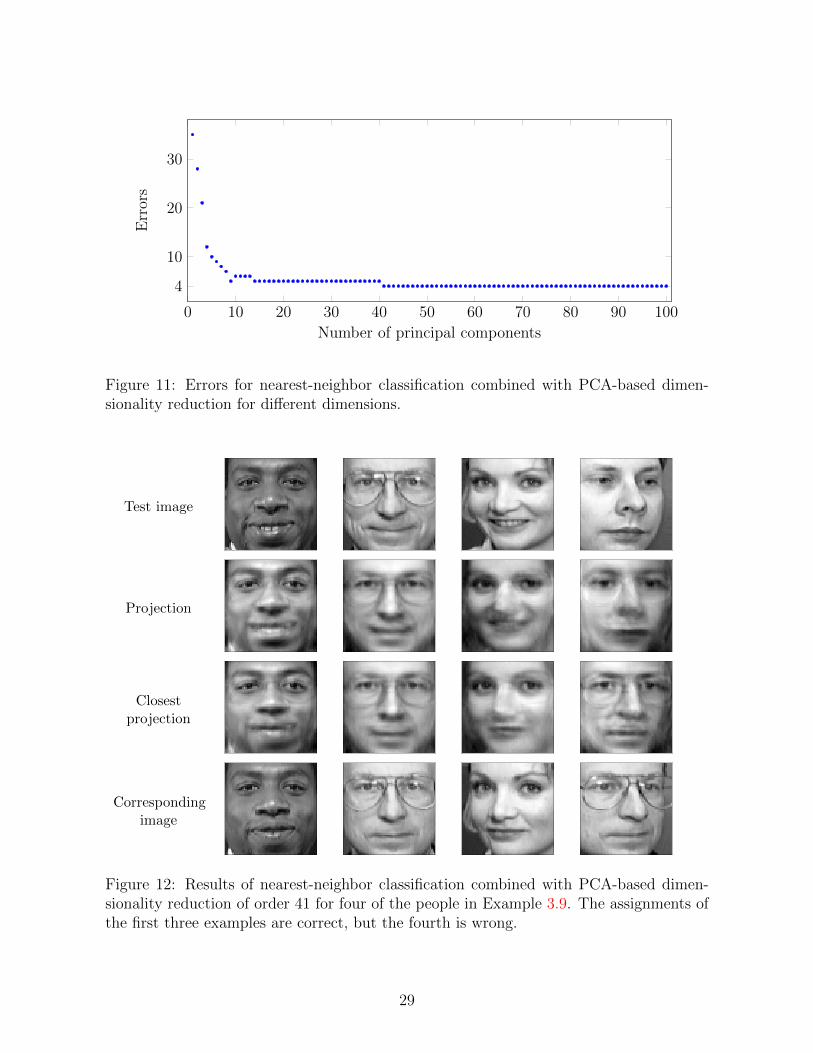
Figure 11: Errors for nearest-neighbor classification combined with PCA-based dimen-sionality reduction for different dimensions.

Test image

Projection

Closestprojection

Correspondingimage

Figure 12: Results of nearest-neighbor classification combined with PCA-based dimen-sionality reduction of order 41 for four of the people in Example 3.9. The assignments ofthe first three examples are correct, but the fourth is wrong.

29

First two PCs Last two PCs

2.5 2.0 1.5 1.0 0.5 0.0 0.5 1.0 1.5 2.0

Projection onto first PC

2.5

2.0

1.5

1.0

0.5

0.0

0.5

1.0

1.5

2.0Pro

ject

ion o

nto

seco

nd P

C

2.5 2.0 1.5 1.0 0.5 0.0 0.5 1.0 1.5 2.0

Projection onto (d-1)th PC

2.5

2.0

1.5

1.0

0.5

0.0

0.5

1.0

1.5

2.0

Pro

ject

ion o

nto

dth

PC

Figure 13: Projection of 7-dimensional vectors describing different wheat seeds onto thefirst two (left) and the last two (right) principal dimensions of the data set. Each colorrepresents a variety of wheat.

If we have to classify a large number of points (i.e. p � max {m,n}) the computationalcost is reduced by operating in the lower-dimensional space.

Figure 11 shows the accuracy of the algorithm on the same data as Example 4.3 in LectureNotes 1. The accuracy increases with the dimension at which the algorithm operates. Thisis not necessarily always the case because projections may actually be helpful for taskssuch as classification (for example, factoring out small shifts and deformations). The sameprecision as in the ambient dimension (4 errors out of 40 test images) is achieved usingjust k = 41 principal components (in this example n = 360 and m = 4096). Figure 12shows some examples of the projected data represented in the original m-dimensionalspace along with their nearest neighbors in the k-dimensional space. 4

Example 3.10 (Dimensionality reduction for visualization). Dimensionality reduction isoften useful for visualization. The objective is to project the data onto 2D or 3D in away that preserves its structure as much as possible. In this example, we consider a dataset where each data point corresponds to a seed with seven features: area, perimeter,compactness, length of kernel, width of kernel, asymmetry coefficient and length of kernelgroove. The seeds belong to three different varieties of wheat: Kama, Rosa and Canadian.2

To visualize the data in 2D, we project each point onto the two first principal dimensionsof the data set.

Figure 13 shows the projection of the data onto the first two and the last two principaldirections. In the latter case, there is almost no discernible variation. As predicted byour theoretical analysis of PCA, the structure in the data is much better conserved by thetwo first directions, which allow to clearly visualize the difference between the three typesof seeds. Note however that projection onto the first principal directions only ensures

2The data can be found at https://archive.ics.uci.edu/ml/datasets/seeds.

30

~x1, . . . , ~xn UT~x1, . . . , UT~xn S−1UT~x1, . . . , S−1UT~xn

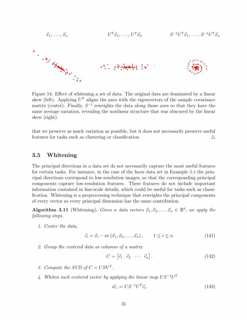
Figure 14: Effect of whitening a set of data. The original data are dominated by a linearskew (left). Applying UT aligns the axes with the eigenvectors of the sample covariancematrix (center). Finally, S−1 reweights the data along those axes so that they have thesame average variation, revealing the nonlinear structure that was obscured by the linearskew (right).

that we preserve as much variation as possible, but it does not necessarily preserve usefulfeatures for tasks such as clustering or classification. 4

3.5 Whitening

The principal directions in a data set do not necessarily capture the most useful featuresfor certain tasks. For instance, in the case of the faces data set in Example 3.4 the prin-cipal directions correspond to low-resolution images, so that the corresponding principalcomponents capture low-resolution features. These features do not include importantinformation contained in fine-scale details, which could be useful for tasks such as classi-fication. Whitening is a preprocessing technique that reweights the principal componentsof every vector so every principal dimension has the same contribution.

Algorithm 3.11 (Whitening). Given n data vectors ~x1, ~x2, . . . , ~xn ∈ Rd, we apply thefollowing steps.

1. Center the data,

~ci = ~xi − av (~x1, ~x2, . . . , ~xn) , 1 ≤ i ≤ n. (141)

2. Group the centered data as columns of a matrix

C =[~c1 ~c2 · · · ~cn

]. (142)

3. Compute the SVD of C = USV T .

4. Whiten each centered vector by applying the linear map US−1UT

~wi := US−1UT~ci. (143)

31

~x

US−1UT~x

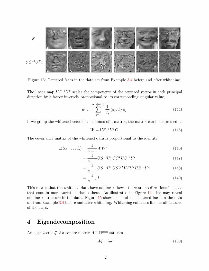
Figure 15: Centered faces in the data set from Example 3.4 before and after whitening.

The linear map US−1UT scales the components of the centered vector in each principaldirection by a factor inversely proportional to its corresponding singular value,

~wi :=

min(m,n)∑j=1

1

σj〈~uj,~ci〉 ~uj. (144)

If we group the whitened vectors as columns of a matrix, the matrix can be expressed as

W = US−1UTC. (145)

The covariance matrix of the whitened data is proportional to the identity

Σ (~c1, . . . ,~cn) =1

n− 1WW T (146)

=1

n− 1US−1UTCCTUS−1UT (147)

=1

n− 1US−1UTUSV TV SUTUS−1UT (148)

=1

n− 1I, (149)

This means that the whitened data have no linear skews, there are no directions in spacethat contain more variation than others. As illustrated in Figure 14, this may revealnonlinear structure in the data. Figure 15 shows some of the centered faces in the dataset from Example 3.4 before and after whitening. Whitening enhances fine-detail featuresof the faces.

4 Eigendecomposition

An eigenvector ~q of a square matrix A ∈ Rn×n satisfies

A~q = λ~q (150)

32

for a scalar λ which is the corresponding eigenvalue. Even if A is real, its eigenvectorsand eigenvalues can be complex. If a matrix has n linearly independent eigenvectors thenit is diagonalizable.

Lemma 4.1 (Eigendecomposition). If a square matrix A ∈ Rn×n has n linearly inde-pendent eigenvectors ~q1, . . . , ~qn with eigenvalues λ1, . . . , λn it can be expressed in terms ofa matrix Q, whose columns are the eigenvectors, and a diagonal matrix containing theeigenvalues,

A =[~q1 ~q2 · · · ~qn

] λ1 0 · · · 00 λ2 · · · 0

· · ·0 0 · · · λn

[~q1 ~q2 · · · ~qn]−1

(151)

= QΛQ−1 (152)

Proof.

AQ =[A~q1 A~q2 · · · A~qn

](153)

=[λ1~q1 λ2~q2 · · · λ2~qn

](154)

= QΛ. (155)

If the columns of a square matrix are all linearly independent, then the matrix has aninverse, so multiplying the expression by Q−1 on both sides completes the proof.

Lemma 4.2. Not all matrices have an eigendecomposition.

Proof. Consider the matrix [0 10 0

]. (156)

Assume an eigenvector ~q associated to an eigenvalue λ, then[~q [2]

0

]=

[0 10 0

] [~q [1]~q [2]

]=

[λ~q [1]λ~q [2]

], (157)

which implies that ~q [2] = 0 and ~q [1] = 0, so the matrix does not have eigenvectorsassociated to nonzero eigenvalues.

Symmetric matrices are always diagonalizable.

Theorem 4.3 (Spectral theorem for symmetric matrices). If A ∈ Rn is symmetric, thenit has an eigendecomposition of the form

A = UΛUT (158)

where the matrix of eigenvectors U is an orthogonal matrix.

33

This is a fundamental result in linear algebra that can be used to prove Theorem 2.1. Werefer to any graduate-level linear-algebra text for the proof.

Together, Theorems 2.1 and 4.3 imply that the SVD A = USV T and the eigendecomposi-tion A = UΛUT of a symmetric matrix are almost the same. The left singular vectors canbe taken to be equal to the eigenvectors. Nonnegative eigenvalues are equal to the singularvectors, and their right singular vectors are equal to the corresponding eigenvectors. Thedifference is that if an eigenvalue λi corresponding to an eigenvector ~ui is negative, thenσi = −λi and the corresponding right-singular vector ~vi = −~ui.A useful application of the eigendecomposition is computing successive matrix products.Assume that we are interested in computing

AA · · ·A~x = Ak~x, (159)

i.e., we want to apply A to ~x k times. Ak cannot be computed by taking the powerof its entries (try out a simple example to convince yourself). However, if A has aneigendecomposition,

Ak = QΛQ−1QΛQ−1 · · ·QΛQ−1 (160)

= QΛkQ−1 (161)

= Q

λk1 0 · · · 00 λk2 · · · 0

· · ·0 0 · · · λkn

Q−1, (162)

using the fact that for diagonal matrices applying the matrix repeatedly is equivalent totaking the power of the diagonal entries. This allows to compute the k matrix productsusing just 3 matrix products and taking the power of n numbers.

Let A ∈ Rn×n be a matrix with eigendecomposition QΛQ−1 and let ~x be an arbitraryvector in Rn. Since the eigenvectors are linearly independent, they form a basis for Rn,so we can represent ~x as

~x =n∑

i=1

αi~qi, αi ∈ R, 1 ≤ i ≤ n. (163)

Now let us apply A to ~x k times,

Ak~x =n∑

i=1

αiAk~qi (164)

=n∑

i=1

αiλki ~qi. (165)

If we assume that the eigenvectors are ordered according to their magnitudes and thatthe magnitude of one of them is larger than the rest, |λ1| > |λ2| ≥ . . ., and that α1 6= 0

34

~q1

~x1~q2

~q1

~x2

~q2

~q1

~x3

~q2

Figure 16: Illustration of the first three iterations of the power method for a matrix witheigenvectors ~q1 and ~q2, with corresponding eigenvalues λ1 = 1.05 and λ2 = 0.1661.

(which happens with high probability if we draw a random ~x) then as k grows larger theterm α1λ

k1~q1 dominates. The term will blow up or tend to zero unless we normalize every

time before applying A. Adding the normalization step to this procedure results in thepower method or power iteration, an algorithm for estimating the eigenvector of a matrixthat corresponds to the largest eigenvalue.

Algorithm 4.4 (Power method).Set ~x1 := ~x/ ||~x||2, where the entries of ~x are drawn at random. For i = 1, 2, 3, . . .,compute

~xi :=A~xi−1||A~xi−1||2

. (166)

Figure 16 illustrates the power method on a simple example, where the matrix is equal to

A =

[0.930 0.3880.237 0.286

]. (167)

The convergence to the eigenvector corresponding to the eigenvalue with the largest mag-nitude is very fast.

We end this section with an example that applies a decomposition to analyze the evolutionof the populations of two animals.

Example 4.5 (Deer and wolfs). A biologist is studying the populations of deer and wolfsin Yellowstone. She concludes that a reasonable model for the populations in year n+ 1is the linear system of equations

dn+1 =5

4dn −

3

4wn, (168)

wn+1 =1

4dn +

1

4wn, n = 0, 1, 2, . . . (169)

where dn and wn denote the number of deer and wolfs in year n. She is interested indetermining the evolution of the populations in the future so she computes an eigende-

35

0 2 4 6 8 10Year

0

200

400

600

800

1000

1200

1400

1600

Popula

tion

0 2 4 6 8 10Year

0

20

40

60

80

100

Popula

tion

0 2 4 6 8 10Year

0

20

40

60

80

100

Popula

tion

Deer

Wolfs

Figure 17: Evolution of the populations of deer and wolfs for different initial populationsin Example 4.5.

composition of the matrix

A :=

[5/4 −3/41/4 1/4

](170)

=

[3 11 1

] [1 00 0.5

] [3 11 1

]−1:= QΛQ−1. (171)

If we denote the initial populations of deer and wolfs as d0 and w0 respectively, thepopulations in year n are given by[

dnwn

]= QΛnQ−1

[d0w0

](172)

=

[3 11 1

] [1 00 0.5n

] [0.5 −0.5−0.5 1.5

] [d0w0

](173)

=d0 − w0

2

[31

]+

3w0 − d08n

[11

]. (174)

As n→∞, if the number of deer is larger than the number of wolfs, then the populationof deer will converge to be three times the population of wolfs, which will converge to ahalf of the difference between their original populations. Since the populations cannot benegative, if the original population of wolfs is larger than that of deer, then both specieswill go extinct. This is confirmed by the simulations shown in Figure 17. 4

5 Proofs

5.1 Proof of Theorem 1.3

It is sufficient to prove

dim (row (A)) ≤ dim (col (A)) (175)

36

for any arbitrary matrix A. Since the row space of A is equal to the column space of AT

and vice versa, applying (175) to AT yields dim (row (A)) ≥ dim (col (A)) which completesthe proof.

To prove (175) let r := dim (row (A)) and let ~x1, . . . , ~xr be a basis for row (A). Consider thevectors A~x1, . . . , A~xr. They belong to col (A) by (11), so if they are linearly independentthen dim (col (A)) ≥ r. We prove that this is the case by contradiction.

Assume that A~x1, . . . , A~xr are linearly dependent. Then there exist scalar coefficientsα1, . . . , αr such that

~0 =r∑

i=1

αiA~xi = A

(r∑

i=1

αi~xi

)by linearity of the matrix product, (176)

This implies that∑r

i=1 αi~xi is orthogonal to every row of A and hence to every vectorin row (A). However it is in the span of a basis of row (A) by construction! This is onlypossible if

∑ri=1 αi~xi = 0, which is a contradiction because ~x1, . . . , ~xr are assumed to be

linearly independent.

5.2 Proof of Lemma 2.9

Let ~a1,~a2, . . . ,~ad1 be a basis for the first subspace and~b1, ~b2, . . . , ~bd2 a basis for the second.

Because the dimension of the vector space is n, the set of vectors ~a1, . . . , ~ad1 ,~b1, . . . , ~bd2

are not linearly independent. There must exist scalars α1, . . . , αd1 , β1, . . . , βd2 , whichare not all equal to zero, such that

d1∑i=1

αi~ai +

d2∑j=1

βi~bi = 0. (177)

The vector

~x :=

d1∑i=1

αi~ai = −d2∑j=1

βi~bi (178)

cannot equal zero because both ~a1, . . . , ~ad1 and ~b1, . . . , ~bd2 are bases by assumption. ~xbelongs to the intersection of the two subspaces, which completes the proof.

5.3 Proof of Theorem 2.16

The proof relies on the following lemma.

Lemma 5.1. For any Q ∈ Rn×n

max1≤i≤n

|Qii| ≤ ||Q|| . (179)

37

Proof. Since ||~ei||2 = 1,

max1≤i≤n

|Qii| ≤ max1≤i≤n

√√√√ n∑j=1

Q2ji (180)

= max1≤i≤n

||Q~ei||2 (181)

≤ ||Q|| . (182)

We denote the SVD of A by USV T ,

sup{||B||≤1 | B∈Rm×n}

tr(ATB

)= sup{||B||≤1 | B∈Rm×n}

tr(V S UTB

)(183)

= sup{||B||≤1 | B∈Rm×n}

tr(S BUTV

)by Lemma 2.5 in Lecture Notes 1

≤ sup{||M ||≤1 |M∈Rm×n}

tr (SM) ||B|| =∣∣∣∣BUTV

∣∣∣∣ by Corollary 2.15

≤ sup{max1≤i≤n|Mii|≤1 |M∈Rm×n}

tr (SM) by Lemma 5.1

≤ sup{max1≤i≤n|Mii|≤1 |M∈Rm×n}

n∑i=1

Mii σi (184)

≤n∑

i=1

σi (185)

= ||A||∗ . (186)

To complete the proof, we need to show that the equality holds. Note that UV T hasoperator norm equal to one because its r singular values (recall that r is the rank of A)are equal to one. We have⟨

A,UV T⟩

= tr(ATUV T

)(187)

= tr(V S UTUV T

)(188)

= tr(V TV S

)by Lemma 2.5 in Lecture Notes 1 (189)

= tr (S) (190)

= ||A||∗ . (191)

38