Lecture Image Enhancement and Spatial Filtering Harvey Rhody Chester F. Carlson Center for Imaging Science Rochester Institute of Technology [email protected] September 29, 2005 Abstract Applications of point processing to image segmentation by global and regional segmentation are constructed and demonstrated. An adaptive threshold algorithm is presented. Illumination compensation is shown to improve global segmentation. Finally, morphological waterfall region segmentation is demonstrated. DIP Lecture 7

Welcome message from author
This document is posted to help you gain knowledge. Please leave a comment to let me know what you think about it! Share it to your friends and learn new things together.
Transcript
Lecture Image Enhancement and SpatialFiltering
Harvey RhodyChester F. Carlson Center for Imaging Science
Rochester Institute of [email protected]
September 29, 2005
AbstractApplications of point processing to image segmentation by global
and regional segmentation are constructed and demonstrated. Anadaptive threshold algorithm is presented. Illumination compensationis shown to improve global segmentation. Finally, morphologicalwaterfall region segmentation is demonstrated.
DIP Lecture 7

Spatial FilteringUses of spatial filtering
• Image enhancement
• Feature detection.
Spatial filtering may be:
• Linear
• Nonlinear
• Spatially invariant
• Spatially varying
DIP Lecture 7 1
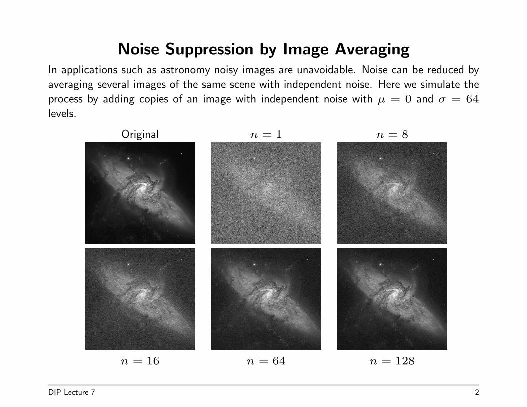
Noise Suppression by Image AveragingIn applications such as astronomy noisy images are unavoidable. Noise can be reduced by
averaging several images of the same scene with independent noise. Here we simulate the
process by adding copies of an image with independent noise with µ = 0 and σ = 64
levels.
Original n = 1 n = 8
n = 16 n = 64 n = 128
DIP Lecture 7 2

Effect of Averaging
Shown at the right is the histogram of the pixel noise
after 8, 16, 64 and 128 images have been averaged.
The standard deviation, which is proportional to the
width of each curve, is reduced by√
n. The reduction
factors are 2.8, 4, 8, 11.3 for n = 8, 16, 64, 128,
respectively.
Averaging is clearly a very effective tool for the reduction of noise provided that enough
independent samples are available.
DIP Lecture 7 3

Region Averaging
Suppose that only a single noisy image is available. Can averaging still be employed for
noise reduction?
Strategy:Average the noise from pixels in a neighborhood.
This necessarily involves averaging of the image as well as the noise.
DIP Lecture 7 4
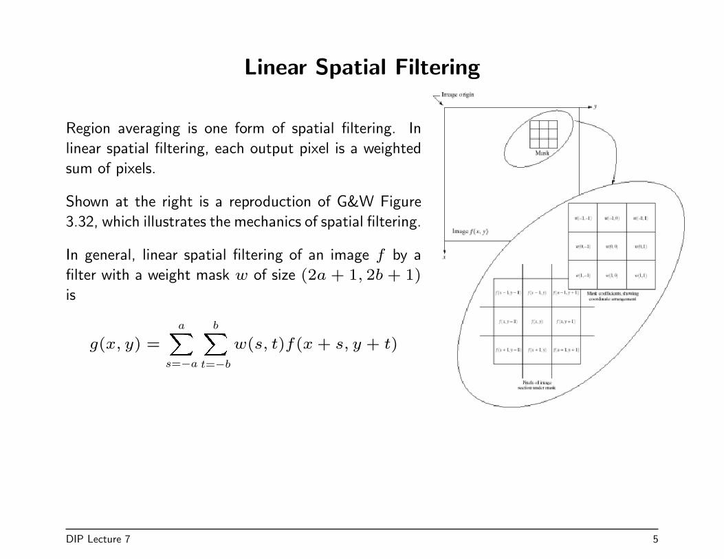
Linear Spatial Filtering
Region averaging is one form of spatial filtering. In
linear spatial filtering, each output pixel is a weighted
sum of pixels.
Shown at the right is a reproduction of G&W Figure
3.32, which illustrates the mechanics of spatial filtering.
In general, linear spatial filtering of an image f by a
filter with a weight mask w of size (2a + 1, 2b + 1)
is
g(x, y) =
aXs=−a
bXt=−b
w(s, t)f(x + s, y + t)
DIP Lecture 7 5

Filters
A linear spatially invariant filter can be represented with a mask that is convolved with the
image array. The weights are represented by the values wi.
w1 w2 w3
w4 w5 w6
w7 w8 w9
If the gray levels of the pixels under the mask are denoted by z1, z2, . . . , z9 then the
response of the linear mask is the sum
R = w1z1 + w2z2 + · · ·+ w9z9
The result R is written to the output array at the position of the filter origin (usually the
center of the filter).
DIP Lecture 7 6

Smoothing Filters
Smoothing filters are used for blurring and noise reduction.
Blurring is a common preprocessing step to remove small details when the objective is
location of large objects.
High-frequency noise is reduced by the lowpass characteristic of smoothing filters.
Smoothing filters have all positive weights. The weights are typically chosen to sum to
unity so that the average brightness values is maintained.
19×
1 1 1
1 1 1
1 1 1
125×
1 1 1 1 1
1 1 1 1 1
1 1 1 1 1
1 1 1 1 1
1 1 1 1 1
149×
1 1 1 1 1 1 1
1 1 1 1 1 1 1
1 1 1 1 1 1 1
1 1 1 1 1 1 1
1 1 1 1 1 1 1
1 1 1 1 1 1 1
1 1 1 1 1 1 1
DIP Lecture 7 7

Smoothing Filters
Smoothing filters calculate a weighted average of the pixels under the mask. The low
frequency response becomes more pronounced as the filter size is increased.
Masks are usually chosen to have odd dimensions to provide a center pixel location. The
output is written to that pixel.
Larger filters do more smoothing but also produce more blurring. An example is shown
below.
Original Image Noisy Image 3× 3 smoothing 5× 5 smoothing
DIP Lecture 7 8

Smoothing Filters
Smoothing is linear and spatially invariant. It is equivalent to convolution of the image
and the mask.
In the frequency domain this is equivalent to multiplication of the image transform with
the mask transform.
The frequency response of smoothing filters of several sizes is shown below. The frequency
range is in normalized units.
Note how the frequency response becomes narrower as the smoothing filter becomes larger.
DIP Lecture 7 9

Frequency Response of Smoothing Filters
M=3 M=5
M=7 M=9
DIP Lecture 7 10
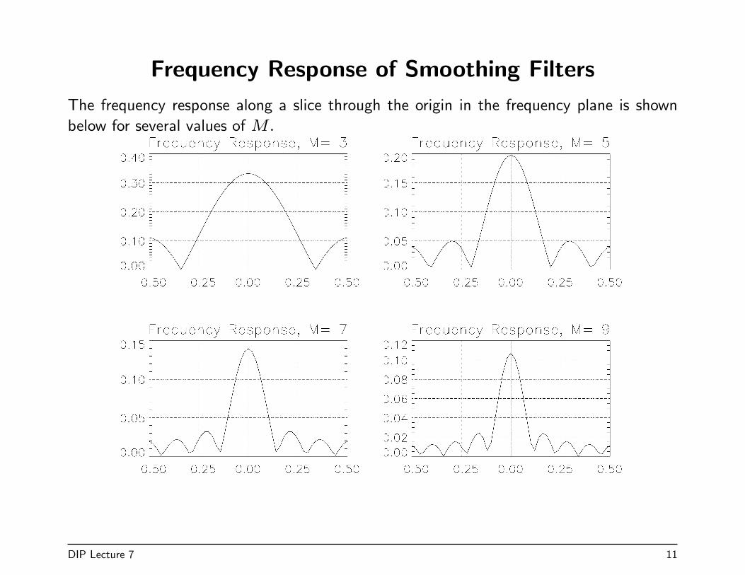
Frequency Response of Smoothing Filters
The frequency response along a slice through the origin in the frequency plane is shown
below for several values of M.
DIP Lecture 7 11

Filter Design
The larger smoothing filters remove more high-frequency energy. This removes more of
the noise and it also removes detail information from edges and other image features.
Averaging filters can emphasize some pixels more than others. Here is a mask that
emphasizes the center pixels more than the edges.
1
25×
1 1 2 1 1
1 2 3 2 1
2 3 4 3 2
1 2 3 2 1
1 1 2 1 1
DIP Lecture 7 12
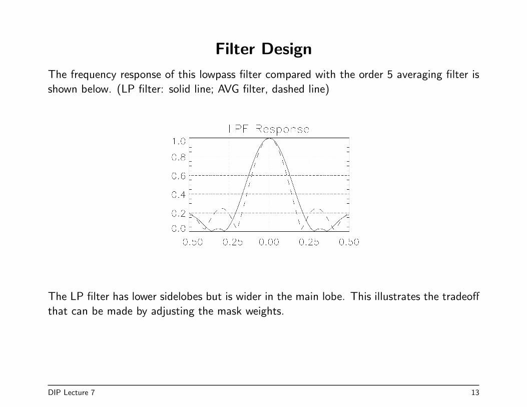
Filter Design
The frequency response of this lowpass filter compared with the order 5 averaging filter is
shown below. (LP filter: solid line; AVG filter, dashed line)
The LP filter has lower sidelobes but is wider in the main lobe. This illustrates the tradeoff
that can be made by adjusting the mask weights.
DIP Lecture 7 13

Filtered Images
The effect of the lowpass filter compared with the order 5 averaging filter is illustrated
below with filtered noisy images. The LP filter has a slightly broader frequency response,
which shows up as slightly less blurring in the right-hand picture.
Averaging Filter Lowpass Filter
DIP Lecture 7 14
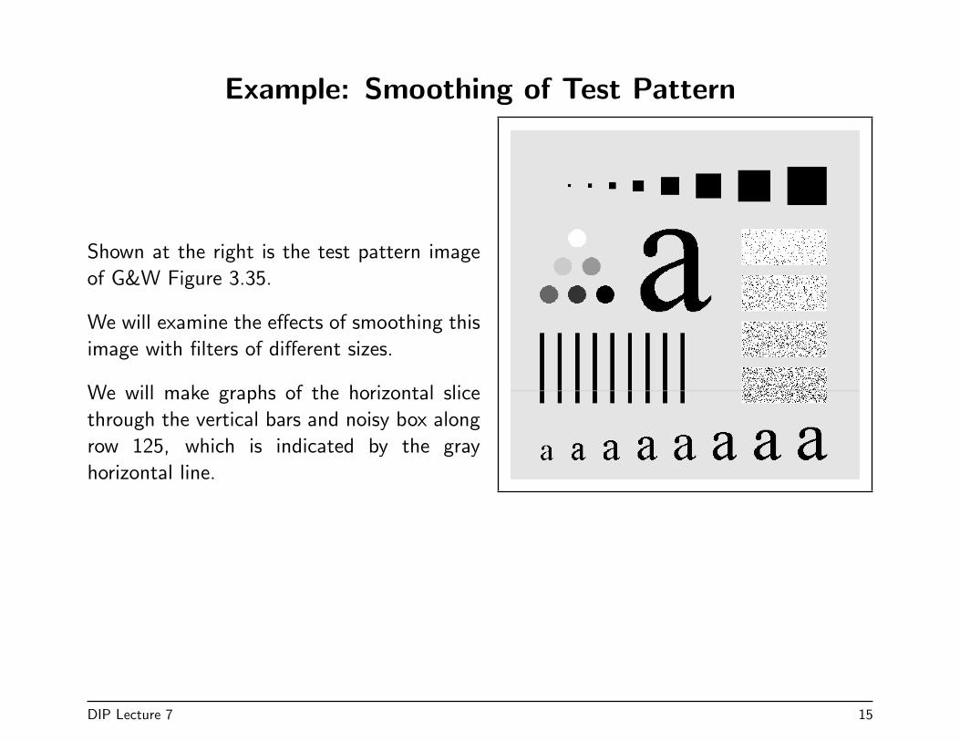
Example: Smoothing of Test Pattern
Shown at the right is the test pattern image
of G&W Figure 3.35.
We will examine the effects of smoothing this
image with filters of different sizes.
We will make graphs of the horizontal slice
through the vertical bars and noisy box along
row 125, which is indicated by the gray
horizontal line.
DIP Lecture 7 15

Smoothing Filter of Size 3× 3
(Right Top) original image; (Right Bottom) result
of smoothing with a 3 × 3 filter; (Below) Plots
along row 125 (top) entire row, (middle) a section
of the vertical bars, (bottom) a section of the noisy
box.
DIP Lecture 7 16
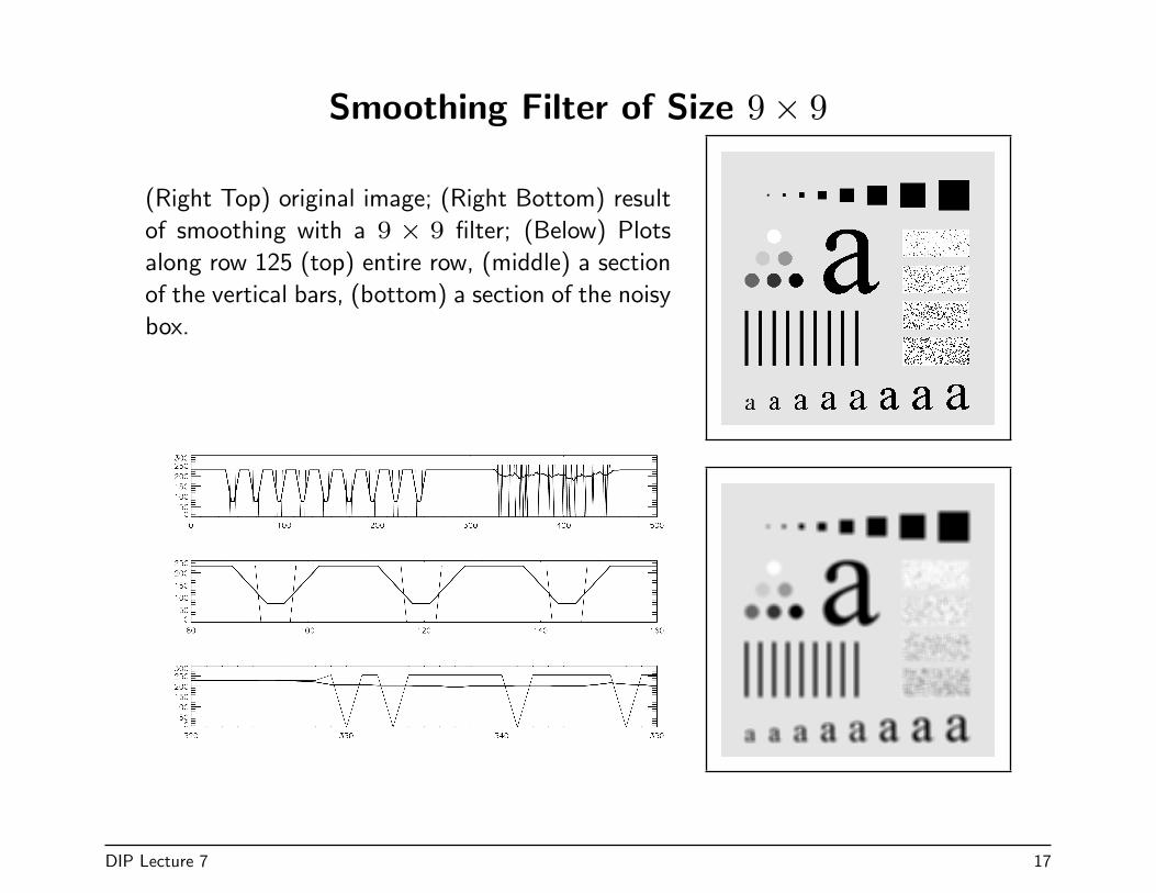
Smoothing Filter of Size 9× 9
(Right Top) original image; (Right Bottom) result
of smoothing with a 9 × 9 filter; (Below) Plots
along row 125 (top) entire row, (middle) a section
of the vertical bars, (bottom) a section of the noisy
box.
DIP Lecture 7 17
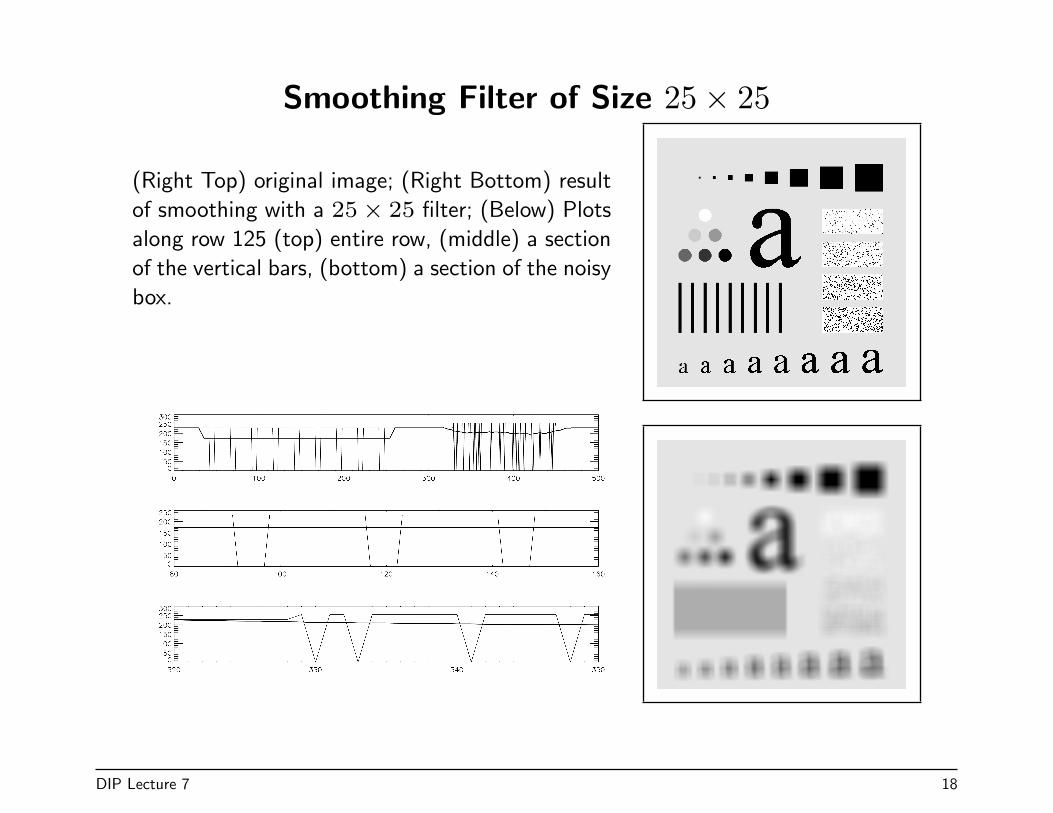
Smoothing Filter of Size 25× 25
(Right Top) original image; (Right Bottom) result
of smoothing with a 25× 25 filter; (Below) Plots
along row 125 (top) entire row, (middle) a section
of the vertical bars, (bottom) a section of the noisy
box.
DIP Lecture 7 18

Smoothing Filter of Size 35× 35
(Right Top) original image; (Right Bottom) result
of smoothing with a 35× 35 filter; (Below) Plots
along row 125 (top) entire row, (middle) a section
of the vertical bars, (bottom) a section of the noisy
box.
DIP Lecture 7 19
Programming
Linear filtering programs are quite easy to write in IDL by using the built-in function,
CONVOL. When all of the filter weights are equal then one can use the function,
SMOOTH.
It is worthwhile using these functions because they run much faster than any user functions
that would be written in IDL.
CONVOL is related to mathematical convolution and to filter weighting. How it works
depends upon the choices of some keyword parameters.
DIP Lecture 7 20

CONVOL
The CONVOL function convolves an array with a kernel, and returns the result. If A
is an N × M array and K is a n × m kernel, with n < N and m < M , then
B=CONVOL(A,K,S) computes an output array B by
B[t, u] =1
S
n−1Xi=0
m−1Xj=0
A[t + i− n/2, u + j −m/2]K[i, j]
Example 1: B=CONVOL(A,K,1) where
A =
26666666664
0 0 0 0 0 0 0
0 0 0 0 0 0 0
0 0 1 0 0 0 0
0 0 0 0 0 0 0
0 0 0 0 0 0 0
0 0 0 0 0 0 0
0 0 0 0 0 0 0
37777777775
and K =
24
1 2 3
4 5 6
7 8 9
35
DIP Lecture 7 21

Example 1 (cont)
Since n = m = 3 we have n/2 = m/2 = 1 (integer division). Since A is zero
everywhere except A[2, 2] = 1 we can write A[r, s] = δ[r − 2, s− 2]. Then
A[t + i− 1, u + j − 1] = δ[t + i− 3, u + j − 3]
so that
B[t, u] =
2Xi=0
2Xj=0
δ[t + i− 3, u + j − 3]K[i, j] = K[3− t, 3− u]
A =
26666666664
0 0 0 0 0 0 0
0 0 0 0 0 0 0
0 0 1 0 0 0 0
0 0 0 0 0 0 0
0 0 0 0 0 0 0
0 0 0 0 0 0 0
0 0 0 0 0 0 0
37777777775
K =
24
1 2 3
4 5 6
7 8 9
35⇒ B =
26666666664
0 0 0 0 0 0 0
0 9 8 7 0 0 0
0 6 5 4 0 0 0
0 3 2 1 0 0 0
0 0 0 0 0 0 0
0 0 0 0 0 0 0
0 0 0 0 0 0 0
37777777775
DIP Lecture 7 22

Example 1 (cont)
The result B contains the kernel pattern, reversed in rows and columns, and centered on
the location of the “impulse” in the array A.
The kernel is reversed in the result because it is not reversed in the equation, as it would
be with true convolution.
Mathematical convolution is carried out by unsetting the CENTER keyword.
C=C0NVOL(A,K,S,CENTER=0) with S=1 produces
A =
26666666664
0 0 0 0 0 0 0
0 0 0 0 0 0 0
0 0 1 0 0 0 0
0 0 0 0 0 0 0
0 0 0 0 0 0 0
0 0 0 0 0 0 0
0 0 0 0 0 0 0
37777777775
K =
24
1 2 3
4 5 6
7 8 9
35⇒ B =
26666666664
0 0 0 0 0 0 0
0 0 0 0 0 0 0
0 0 1 2 3 0 0
0 0 4 5 6 0 0
0 0 7 8 9 0 0
0 0 0 0 0 0 0
0 0 0 0 0 0 0
37777777775
DIP Lecture 7 23

CONVOL with CENTER=0
When the keyword CENTER is explicitly set to zero, then the equation computed by the
routine is (in 2D)
C[t, u] =
n−1Xi=0
m−1Xj=0
A[t− i, u− j]K[i, j]
In the case A[r, s] = δ[r − 2, s− 2] we have
C[t, u] =
n−1Xi=0
m−1Xj=0
δ[t− i− 2, s− j − 2]K[i, j] = K[t− 2, s− 2]
The result has the kernel “unflipped” but shifted so that its corner is in the position of the
impulse in A.
DIP Lecture 7 24

Using CONVOL
CONVOL uses the keywords CENTER, EDGE TRUNCATE, and EDGE WRAP to control
the computation. We will do several computation examples in class to illustrate the
different results.
The result returned by CONVOL is always of the same size as the input array, namely,
N × M . True convolution produces an output of size N + n − 1, M + m − 1. It
is necessary to use zero-padding to achieve this result. This will be discussed further in
connection with the FFT.
The kernel must be smaller than the array.
DIP Lecture 7 25
SMOOTH
The IDL function SMOOTH implements a strictly uniform kernel. It is useful to achieve
uniform smoothing.
The code has been written to take advantage of the uniform kernel, which makes it faster
than CONVOL.
DIP Lecture 7 26

Discrete 1D Convolution
Let f(x) be defined for x = 0, 1, 2, . . . , A − 1 and h(x) be defined forx = 0, 1, 2, . . . , B − 1. Let M be an integer such that
M ≥ A + B − 1
Let fe(x) and he(x) be extended by zero padding such that
fe(x) ={
f(x) 0 ≤ x ≤ A− 10 A < x ≤ M − 1
he(x) ={
h(x) 0 ≤ x ≤ B − 10 B < x ≤ M − 1
for the interval 0 ≤ x ≤ M − 1. Then extend fe(x) and he(x) for allintegers x by repeating the basic interval with period M .
DIP Lecture 7 1
Discrete 1D Convolution (cont)
fe(x + kM) = fe(x)
he(x + kM) = he(x)
Then the discrete convolution of f and h is
g(x) = f ? h =M−1∑m=0
fe(x)he(m− x)
Note that g(x) is periodic with period M and is defined for all x ∈ Z. Howwould you show that?
DIP Lecture 7 2

Matrix Expression for 1D Convolution
The main period of g(x), 0 ≤ x ≤ M − 1 can be computed by
g = Hf
where g and f are column vectors of length M and H is a M ×M matrix
[g(0)g(1)
...g(M − 1)
]=
he(0) he(−1) he(−2) . . . he(−M + 1)he(1) he(0) he(−1) . . . he(−M + 2)he(2) he(1) he(0) . . . he(−M + 3)
...he(M − 1) he(M − 2) he(M − 3) . . . he(0)
fe(0)fe(1)fe(2)
...fe(M − 1)
By making use of periodicity of he we have the equivalent expression
[g(0)g(1)
...g(M − 1)
]=
he(0) he(M − 1) he(M − 2) . . . he(1)he(1) he(0) he(M − 1) . . . he(2)he(2) he(1) he(0) . . . he(3)
...he(M − 1) he(M − 2) he(M − 3) . . . he(0)
fe(0)fe(1)fe(2)
...fe(M − 1)
Each row of H is a circular shift of the one above. This form is called acirculant matrix.
DIP Lecture 7 3

2D Convolution
In this case f(x, y) and h(x, y) are 2D discrete arrays.
fe(x, y) ={
f(x, y) 0 ≤ x ≤ A− 1 0 ≤ y ≤ B − 10 A ≤ x ≤ M − 1 B ≤ y ≤ N − 1
he(x, y) ={
h(x, y) 0 ≤ x ≤ C − 1 0 ≤ y ≤ D − 10 C < x ≤ M − 1 C ≤ y ≤ N − 1
where M = A+C−1 and N = B+D−1 The function repeats periodicallyin a tiling fashion with tiles of size M ×N .
g(x, y) =M−1∑m=0
N−1∑n=0
fe(m,n)he(x−m, y − n)
DIP Lecture 7 4
Related Documents