Artificial Neural Networks and Pattern Recognition For students of HI 5323 “Image Processing” Willy Wriggers, Ph.D. School of Health Information Sciences http://biomachina.org/courses/processing/13.html T H E U N I V E R S I T Y of T E X A S H E A L T H S C I E N C E C E N T E R A T H O U S T O N S C H O O L of H E A L T H I N F O R M A T I O N S C I E N C E S

Lecture artificial neural networks and pattern recognition
Jun 26, 2015
Welcome message from author
This document is posted to help you gain knowledge. Please leave a comment to let me know what you think about it! Share it to your friends and learn new things together.
Transcript

Artificial Neural Networks and Pattern RecognitionFor students of HI 5323 “Image Processing”
Willy Wriggers, Ph.D.School of Health Information Sciences
http://biomachina.org/courses/processing/13.html
T H E U N I V E R S I T Y of T E X A S
H E A L T H S C I E N C E C E N T E R A T H O U S T O N
S C H O O L of H E A L T H I N F O R M A T I O N S C I E N C E S

Biology

What are Neural Networks?
• Models of the brain and nervous system
• Highly parallelProcess information much more like the brain than a serial computer
• Learning
• Very simple principles
• Very complex behaviours
• ApplicationsAs powerful problem solversAs biological models
© [email protected], users.ox.ac.uk/~quee0818/teaching/Neural_Networks.ppt

Neuro-Physiological Background
• 10 billion neurons in human cortex
• 60 trillion synapses
• In first two years from birth ~1 million synapses / sec. formed
pyramidal cell

Organizing Principle

Various Types of Neurons

Neuron Models

Modeling the Neuron
bias
inputs
h(w0,wi , xi ) y = f h( )y
x1 w1
xiwi
xnwn
1w0 f : activation function
output
h : combine wi & xi
© Leonard Studer, humanresources.web.cern.ch/humanresources/external/training/ tech/special/DISP2003/DISP-2003_L21A_30Apr03.ppt
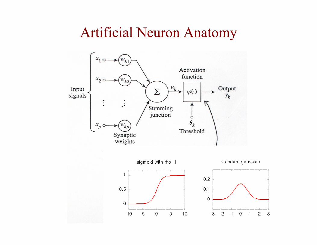
Artificial Neuron Anatomy

Common Activation Functions
• Sigmoidal Function:
• Radial Function, e.g.. Gaussian:
• Linear Function
y = f h = w0 ⋅1+ wi ⋅ xii=1
n
∑ ; ρ⎛
⎝ ⎜
⎞
⎠ ⎟ =
1
1+ e−h
ρ
y = f h = xi − wi( )2
i=1
n
∑ ; σ = w0
⎛
⎝ ⎜
⎞
⎠ ⎟ =
12πσ
e−
h 2
2σ 2
y = w0 ⋅1+ wi ⋅ xii=1
n
∑
© Leonard Studer, humanresources.web.cern.ch/humanresources/external/training/ tech/special/DISP2003/DISP-2003_L21A_30Apr03.ppt

Supervised Learning

Artificial Neural Networks• ANNs incorporate the two fundamental components of
biological neural nets:
1. Neurones (nodes)
2. Synapses (weights)
© [email protected], users.ox.ac.uk/~quee0818/teaching/Neural_Networks.ppt
Input Output

“Pidgeon” ANNs• Pigeons as art experts (Watanabe et al. 1995)
• Experiment:- Pigeon in Skinner box- Present paintings of two different artists (e.g. Chagall / Van Gogh)- Reward for pecking when presented a particular artist (e.g. Van Gogh)
© [email protected], users.ox.ac.uk/~quee0818/teaching/Neural_Networks.ppt

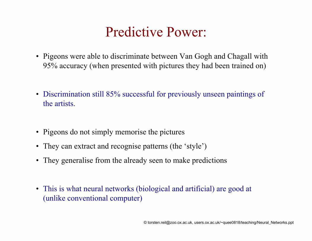
• Pigeons were able to discriminate between Van Gogh and Chagall with 95% accuracy (when presented with pictures they had been trained on)
• Discrimination still 85% successful for previously unseen paintings of the artists.
• Pigeons do not simply memorise the pictures
• They can extract and recognise patterns (the ‘style’)
• They generalise from the already seen to make predictions
• This is what neural networks (biological and artificial) are good at (unlike conventional computer)
© [email protected], users.ox.ac.uk/~quee0818/teaching/Neural_Networks.ppt
Predictive Power:

Real ANN Applications
• Recognition of hand-written letters
• Predicting on-line the quality of welding spots
• Identifying relevant documents in corpus
• Visualizing high-dimensional space
• Tracking on-line the position of robot arms
• … etc
© Leonard Studer, humanresources.web.cern.ch/humanresources/external/training/ tech/special/DISP2003/DISP-2003_L21A_30Apr03.ppt

ANN Design1. Get a large amount of data: inputs and outputs2. Analyze data on the PC
Relevant inputs ?Linear correlations (ANN necessary) ?Transform and scale variablesOther useful preprocessing ?Divide in 3 data sets:
Training setTest setValidation set
© Leonard Studer, humanresources.web.cern.ch/humanresources/external/training/ tech/special/DISP2003/DISP-2003_L21A_30Apr03.ppt

3. Set the ANN architecture: What type of ANN ?Number of inputs, outputs ?Number of hidden layersNumber of neurons Learning schema « details »
4. Tune/optimize internal parameters by presenting training data set to ANN
5. Validate on test / validation dataset
© Leonard Studer, humanresources.web.cern.ch/humanresources/external/training/ tech/special/DISP2003/DISP-2003_L21A_30Apr03.ppt
ANN Design

Main Types of ANNSupervised Learning:
Feed-forward ANN- Multi-Layer Perceptron (with sigmoid hidden neurons)
Recurrent Networks- Neurons are connected to self and others- Time delay of signal transfer- Multidirectional information flow
Unsupervised Learning:
Self-organizing ANN- Kohonen Maps- Vector Quantization - Neural Gas

Feed-Forward ANN
• Information flow is unidirectional• Data is presented to Input layer
• Passed on to Hidden Layer
• Passed on to Output layer
• Information is distributed
• Information processing is parallel
Internal representation (interpretation) of data
© [email protected], users.ox.ac.uk/~quee0818/teaching/Neural_Networks.ppt

Supervised Learning
Training set: {(µxin, µtout);
1 ≤ µ ≤ P}
µ xout
desired output(supervisor) µ t out
µ xin
error=µ xout −µ t out
Typically: backprop. of errors
© Leonard Studer, humanresources.web.cern.ch/humanresources/external/training/ tech/special/DISP2003/DISP-2003_L21A_30Apr03.ppt
-

Important Properties of FFN
• Assumeg(x): bounded and sufficiently regular fct.FFN with 1 hidden layer of finite N neurons (Transfer function is identical for every neurons)
• => FFN is an Universal Approximator of g(x)Theorem by Cybenko et al. in 1989
In the sense of uniform approximation For arbitrary precision ε
© Leonard Studer, humanresources.web.cern.ch/humanresources/external/training/ tech/special/DISP2003/DISP-2003_L21A_30Apr03.ppt

• AssumeFFN as before
(1 hidden layer of finite N neurons, non linear transfer function)
Approximation precision ε
• => #{wi} ~ # inputsTheorem by Barron in 1993
ANN is more parsimonious in #{wi} than a linear approximator[linear approximator: #{wi} ~ exp(# inputs) ]
© Leonard Studer, humanresources.web.cern.ch/humanresources/external/training/ tech/special/DISP2003/DISP-2003_L21A_30Apr03.ppt
Important Properties of FFN
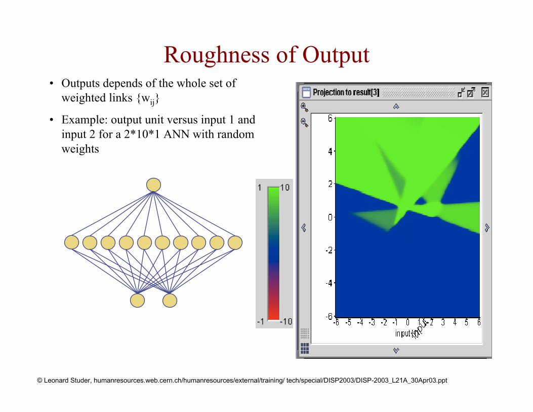
Roughness of Output• Outputs depends of the whole set of
weighted links {wij}
• Example: output unit versus input 1 and input 2 for a 2*10*1 ANN with random weights
© Leonard Studer, humanresources.web.cern.ch/humanresources/external/training/ tech/special/DISP2003/DISP-2003_L21A_30Apr03.ppt

(1 × 0.25) + (0.5 × (-1.5)) = 0.25 + (-0.75) = - 0.5
0.37751
15.0
=+ e
Squashing:
© [email protected], users.ox.ac.uk/~quee0818/teaching/Neural_Networks.ppt
Feeding Data Through the FNN

• Data is presented to the network in the form of activations in the input layer
• ExamplesPixel intensity (for pictures)Molecule concentrations (for artificial nose)Share prices (for stock market prediction)
• Data usually requires preprocessingAnalogous to senses in biology
• How to represent more abstract data, e.g. a name?Choose a pattern, e.g.- 0-0-1 for “Chris”- 0-1-0 for “Becky”
© [email protected], users.ox.ac.uk/~quee0818/teaching/Neural_Networks.ppt
Feeding Data Through the FNN

How do we adjust the weights?
• BackpropagationRequires training set (input / output pairs)Starts with small random weightsError is used to adjust weights (supervised learning)Gradient descent on error landscape
© [email protected], users.ox.ac.uk/~quee0818/teaching/Neural_Networks.ppt
Training the Network


• AdvantagesIt works!Relatively fast
• DownsidesRequires a training setCan be slow to convergeProbably not biologically realistic
• Alternatives to BackpropagationHebbian learning- Not successful in feed-forward nets
Reinforcement learning- Only limited success in FFN
Artificial evolution- More general, but can be even slower than backprop
© [email protected], users.ox.ac.uk/~quee0818/teaching/Neural_Networks.ppt
Backpropagation

Pattern recognition- Character recognition- Face Recognition
Sonar mine/rock recognition (Gorman & Sejnowksi, 1988)
Navigation of a car (Pomerleau, 1989)
Stock-market prediction
Pronunciation (NETtalk)(Sejnowksi & Rosenberg, 1987)
© [email protected], users.ox.ac.uk/~quee0818/teaching/Neural_Networks.ppt
Applications of FFN

Protein Secondary Structure Prediction
(Holley-Karplus, Ph.D., etc):
Supervised learning:Adjust weight vectors so output of network matches desired result
coil
α-helical
amin
o ac
id s
eque
nce
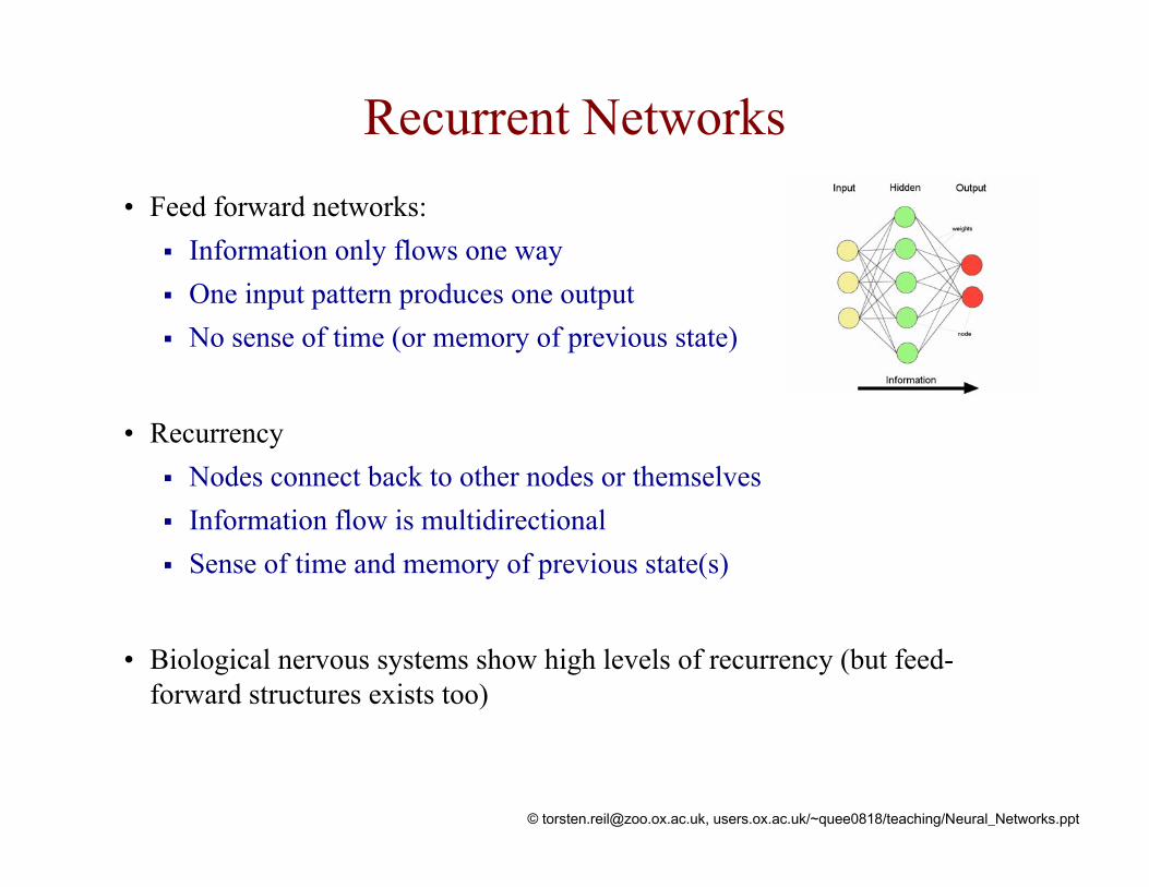
Recurrent Networks• Feed forward networks:
Information only flows one wayOne input pattern produces one outputNo sense of time (or memory of previous state)
• RecurrencyNodes connect back to other nodes or themselvesInformation flow is multidirectionalSense of time and memory of previous state(s)
• Biological nervous systems show high levels of recurrency (but feed-forward structures exists too)
© [email protected], users.ox.ac.uk/~quee0818/teaching/Neural_Networks.ppt

Elman Nets
• Elman nets are feed forward networks with partial recurrency
• Unlike feed forward nets, Elman nets have a memory or sense of time
© [email protected], users.ox.ac.uk/~quee0818/teaching/Neural_Networks.ppt

Classic experiment on language acquisition and processing (Elman, 1990)
• TaskElman net to predict successive words in sentences.
• DataSuite of sentences, e.g.
- “The boy catches the ball.”- “The girl eats an apple.”
Words are input one at a time
• RepresentationBinary representation for each word, e.g.
- 0-1-0-0-0 for “girl”
• Training methodBackpropagation
© [email protected], users.ox.ac.uk/~quee0818/teaching/Neural_Networks.ppt
Elman Nets

© [email protected], users.ox.ac.uk/~quee0818/teaching/Neural_Networks.ppt
Elman Nets
Internal representation of words

Hopfield Networks
• Sub-type of recurrent neural netsFully recurrentWeights are symmetricNodes can only be on or offRandom updating
• Learning: Hebb rule (cells that fire together wire together)
• Can recall a memory, if presented with a
corrupt or incomplete version
auto-associative or
content-addressable memory
© [email protected], users.ox.ac.uk/~quee0818/teaching/Neural_Networks.ppt

Task: store images with resolution of 20x20 pixels
Hopfield net with 400 nodes
Memorise:1. Present image2. Apply Hebb rule (cells that fire together, wire together)
- Increase weight between two nodes if both have same activity, otherwise decrease
3. Go to 1
Recall:1. Present incomplete pattern2. Pick random node, update3. Go to 2 until settled
© [email protected], users.ox.ac.uk/~quee0818/teaching/Neural_Networks.ppt
Hopfield Networks


• Memories are attractors in state space
© [email protected], users.ox.ac.uk/~quee0818/teaching/Neural_Networks.ppt
Hopfield Networks

• Problem: memorising new patterns corrupts the memory of older onesOld memories cannot be recalled, or spurious memories arise
• Solution: allow Hopfield net to sleep
© [email protected], users.ox.ac.uk/~quee0818/teaching/Neural_Networks.ppt
Catastrophic Forgetting

Unlearning (Hopfield, 1986)
- Recall old memories by random stimulation, but use an inverseHebb rule‘Makes room’ for new memories (basins of attraction shrink)
Pseudorehearsal (Robins, 1995)
- While learning new memories, recall old memories by random stimulation
- Use standard Hebb rule on new and old memoriesRestructure memory
• Needs short-term + long term memory- Mammals: hippocampus plays back new memories to neo-cortex,
which is randomly stimulated at the same time
© [email protected], users.ox.ac.uk/~quee0818/teaching/Neural_Networks.ppt
Solutions

Unsupervised Learning

Unsupervised (Self-Organized) Learning
feed-forward (supervised)
feed-forward + lateral feedback(recurrent network, still supervised)
self-organizing network (unsupervised)continuous input space
discrete output space
input layer output layer
input layer output layer

Self Organizing Map (SOM)
neural lattice
input signal space
Kohonen, 1984

Illustration of Kohonen LearningInputs: coordinates (x,y) of points
drawn from a square
Display neuron j at position xj,yj where its sj is maximum
random initial positions
100 inputs 200 inputs
1000 inputs
© Leonard Studer, humanresources.web.cern.ch/humanresources/external/training/ tech/special/DISP2003/DISP-2003_L21A_30Apr03.ppt

• Image Analysis- Image Classification
• Data Visualization- By projection from high D -> 2DPreserving neighborhood relationships
• Partitioning Input SpaceVector Quantization (Coding)
© Leonard Studer, humanresources.web.cern.ch/humanresources/external/training/ tech/special/DISP2003/DISP-2003_L21A_30Apr03.ppt
Why use Kohonen Maps?

Example:Modeling of the somatosensory map of the hand (Ritter, Martinetz &
Schulten, 1992).

Example:Modeling of the somatosensory map of the hand (Ritter, Martinetz &
Schulten, 1992).

Example:Modeling of the somatosensory map of the hand (Ritter, Martinetz &
Schulten, 1992).

Example:Modeling of the somatosensory map of the hand (Ritter, Martinetz &
Schulten, 1992).

Example:Modeling of the somatosensory map of the hand (Ritter, Martinetz &
Schulten, 1992).

Example:Modeling of the somatosensory map of the hand (Ritter, Martinetz &
Schulten, 1992).

Representing Topology with the Kohonen SOM
• free neurons from lattice…
• stimulus–dependent connectivities

The “Neural Gas” Algorithm (Martinetz & Schulten, 1992)
connectivity matrix:Cij { 0, 1}age matrix:Tij {0,…,T}
stimulus

Example

Example (cont.)

More Examples: Torus and Myosin S1
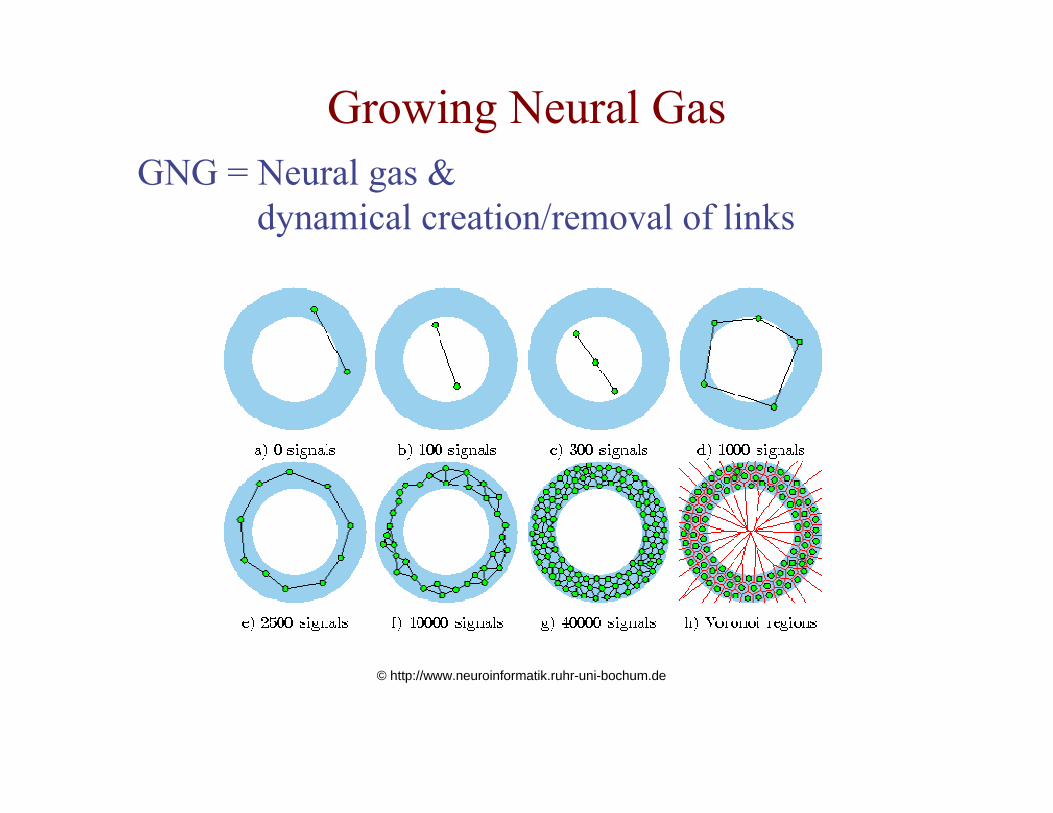
Growing Neural GasGNG = Neural gas &
dynamical creation/removal of links
© http://www.neuroinformatik.ruhr-uni-bochum.de

Why use GNG ?
• Adaptability to Data TopologyBoth dynamically and spatially
• Data Analysis
• Data Visualization
© Leonard Studer, humanresources.web.cern.ch/humanresources/external/training/ tech/special/DISP2003/DISP-2003_L21A_30Apr03.ppt

Radial Basis Function Networks
hidden layer of RBF neurons
Inputs (fan in)
Outputs aslinear
combination of
Usually apply a unsupervised learning procedure
•Set number of neurons and then adjust :
1.Gaussian centers
2.Gaussian widths
3.weights
© Leonard Studer, humanresources.web.cern.ch/humanresources/external/training/ tech/special/DISP2003/DISP-2003_L21A_30Apr03.ppt

Why use RBF ?
• Density estimation
• Discrimination
• Regression
• Good to know:Can be described as Bayesian NetworksClose to some Fuzzy Systems
© Leonard Studer, humanresources.web.cern.ch/humanresources/external/training/ tech/special/DISP2003/DISP-2003_L21A_30Apr03.ppt
Demo
Internet Java demo http://www.neuroinformatik.ruhr-uni-bochum.de/ini/VDM/research/gsn/DemoGNG/GNG.html
• Hebb Rule
• LBG / k-means
• Neural Gas
• GNG
• Kohonen SOM

Revisiting Quantization

Vector QuantizationLloyd (1957)
Linde, Buzo, & Gray (1980)Martinetz & Schulten (1993)
Digital Signal Processing,Speech and Image Compression.Neural Gas.
}
{ }jwEncode data (in ) using a finite set (j=1,…,k) of codebook vectors.DℜDelaunay triangulation divides into k Voronoi polyhedra (“receptive fields”):Dℜ
{ }V Di i jv v w v w j= ∈ ℜ − ≤ − ∀

Vector Quantization

k-Means a.k.a. Linde, Buzo & Gray (LBG)Encoding Distortion Error:
2
(data points)( ) i
i
E di j iv w= −∑
Lower iteratively: Gradient descent( ){ }( )twE j
( ) ( ) ( )( )( ) 1 .2r r r rj i i r i
ir
Ew t w t w t v w dw
ε ε δ∂∆ ≡ − − = − ⋅ = ⋅ −
∂ ∑ :r∀
Inline (Monte Carlo) approach for a sequence selected at random according to propability density function
( )tvi:id
( )( ). ~ )( )( riirjr wtvtw −⋅⋅=∆ δε
Advantage: fast, reasonable clustering.Limitations: depends on initial random positions, difficult to avoid getting trapped in the many local minima of E

Neural Gas Revisited
1 1 0 )1(10
−===
−≤≤−≤− −
ksss
wvwvwv
rrr
kjijiji …
( ) { }( )jir wtvs ,
Avoid local minima traps of k-means by smoothing of energy function:
( )( ) , ~ )( : ri
s
r wtvetwrr
−⋅⋅=∆∀−λε
Where is the closeness rank:

Neural Gas Revisited
{ }( )2k
r 1, .( )
rs
j ii
E w e di j iv wλλ
−
=
= −∑ ∑
Note: k-means.not only “winner” , also second, third, ... closest are updated.
:0→λ:0≠λ ( )ijw
Can show that this corresponds to stochastic gradient descent on
Note: k-means.parabolic (single minimum).
. ~ :0 EE →→λE~ :∞→λ } ( )t λ⇒

Codebook vector variability arises due to:• statistical uncertainty,• spread of local minima.
A small variability indicates good convergence behavior.Optimum choice of # of vectors k: variability is minimal.
Q: How do we know that we have found the global minimum of E?A: We don’t (in general).
But we can compute the statistical variability of the by repeating thecalculation with different seeds for random number generator.
{ }jw
Neural Gas Revisited

Pattern Recognition

Pattern Recognition
• A pattern is an object, process or event that can be given a name.
• A pattern class (or category) is a set of patterns sharing common attributes and usually originating from the same source.
• During recognition (or classification) given objects are assigned to prescribed classes.
• A classifier is a machine which performs classification.
Definition: “The assignment of a physical object or event to one of several prespecified categeries” -- Duda & Hart
© Voitech Franc, cmp.felk.cvut.cz/~xfrancv/talks/franc-printro03.ppt

PR Applications
• Optical Character
Recognition (OCR)
• Biometrics
• Diagnostic systems
• Handwritten: sorting letters by postal code, input device for PDA‘s.• Printed texts: reading machines for blind people, digitalization of text documents.
• Face recognition, verification, retrieval. • Finger prints recognition.• Speech recognition.
• Medical diagnosis: X-Ray, EKG analysis.• Machine diagnostics, waster detection.
© Voitech Franc, cmp.felk.cvut.cz/~xfrancv/talks/franc-printro03.ppt

Approaches
• Statistical PR: based on underlying statistical model of patterns and pattern classes.
• Structural (or syntactic) PR: pattern classes represented by means of formal structures as grammars, automata, strings, etc.
• Neural networks: classifier is represented as a network of cells modeling neurons of the human brain (connectionist approach).
© Voitech Franc, cmp.felk.cvut.cz/~xfrancv/talks/franc-printro03.ppt
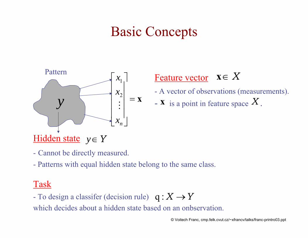
Basic Concepts
y x=
⎥⎥⎥⎥
⎦
⎤
⎢⎢⎢⎢
⎣
⎡
nx
xx
2
1 Feature vector- A vector of observations (measurements).- is a point in feature space .
Hidden state- Cannot be directly measured.- Patterns with equal hidden state belong to the same class.
X∈x
x X
Y∈y
Task- To design a classifer (decision rule) which decides about a hidden state based on an onbservation.
YX →:q
Pattern
© Voitech Franc, cmp.felk.cvut.cz/~xfrancv/talks/franc-printro03.ppt

Example
x=⎥⎦
⎤⎢⎣
⎡
2
1
xx
height
weight
Task: jockey-hoopster recognition.
The set of hidden state is
The feature space is },{ JH=Y
2ℜ=X
Training examples )},(,),,{( 11 ll yy xx …
1x
2x
Jy =
Hy =Linear classifier:
⎩⎨⎧
<+⋅≥+⋅
=0)(0)(
)q(bifJbifH
xwxw
x
0)( =+⋅ bxw
© Voitech Franc, cmp.felk.cvut.cz/~xfrancv/talks/franc-printro03.ppt

Components of a PR System
Sensors and preprocessing
Feature extraction Classifier Class
assignment
• Sensors and preprocessing.• A feature extraction aims to create discriminative features good for classification.• A classifier.• A teacher provides information about hidden state -- supervised learning.• A learning algorithm sets PR from training examples.
Learning algorithmTeacher
Pattern
© Voitech Franc, cmp.felk.cvut.cz/~xfrancv/talks/franc-printro03.ppt

Feature Extraction
Task: to extract features which are good for classification.Good features: • Objects from the same class have similar feature values.
• Objects from different classes have different values.
“Good” features “Bad” features
© Voitech Franc, cmp.felk.cvut.cz/~xfrancv/talks/franc-printro03.ppt

Feature Extraction Methods
⎥⎥⎥⎥
⎦
⎤
⎢⎢⎢⎢
⎣
⎡
km
mm
2
1
⎥⎥⎥⎥
⎦
⎤
⎢⎢⎢⎢
⎣
⎡
nx
xx
2
11φ
2φ
nφ ⎥⎥⎥⎥⎥⎥
⎦
⎤
⎢⎢⎢⎢⎢⎢
⎣
⎡
km
mmm
3
2
1
⎥⎥⎥⎥
⎦
⎤
⎢⎢⎢⎢
⎣
⎡
nx
xx
2
1
Feature extraction Feature selection
Problem can be expressed as optimization of parameters of featrure extractor .
Supervised methods: objective function is a criterion of separability (discriminability) of labeled examples, e.g., linear discriminant analysis (LDA).
Unsupervised methods: lower dimesional representation which preserves important characteristics of input data is sought for, e.g., principal component analysis (PCA).
φ(θ)
© Voitech Franc, cmp.felk.cvut.cz/~xfrancv/talks/franc-printro03.ppt

Classifier
A classifier partitions feature space X into class-labeled regions such that
||21 YXXXX ∪∪∪= … }0{||21 =∩∩∩ YXXX …and
1X 3X
2X
1X1X
2X
3X
The classification consists of determining to which region a feature vector x belongs to.
Borders between decision boundaries are called decision regions.
© Voitech Franc, cmp.felk.cvut.cz/~xfrancv/talks/franc-printro03.ppt

Representation of a Classifier
A classifier is typically represented as a set of discriminant functions
||,,1,:)(f YX …=ℜ→ ii xThe classifier assigns a feature vector x to the i-the class if )(f)(f xx ji > ij ≠∀
)(f1 x
)(f2 x
)(f || xY
maxx yFeature vector
Discriminant function
Class identifier
© Voitech Franc, cmp.felk.cvut.cz/~xfrancv/talks/franc-printro03.ppt

Bayesian Decision Making
• The Bayesian decision making is a fundamental statistical approach which allows to design the optimal classifier if complete statistical model is known.
Definition: Obsevations Hidden statesDecisions
A loss functionA decision rule A joint probability D
DX →:q)p( y,x
XY
RDYW →×:
Task: to design decision rule q which minimizes Bayesian risk
∑∑∈ ∈
=Yy Xx
yy )),W(q(),p(R(q) xx
© Voitech Franc, cmp.felk.cvut.cz/~xfrancv/talks/franc-printro03.ppt

Example of a Bayesian Task
Task: minimization of classification error.
A set of decisions D is the same as set of hidden states Y.
0/1 - loss function used ⎩⎨⎧
≠=
=yifyif
y)q(1)q(0
)),W(q(xx
x
The Bayesian risk R(q) corresponds to probability of misclassification.
The solution of Bayesian task is
)p()p()|p(maxarg)|(maxargR(q)minargq *
q
*
xxx yyypy
yy==⇒=
© Voitech Franc, cmp.felk.cvut.cz/~xfrancv/talks/franc-printro03.ppt
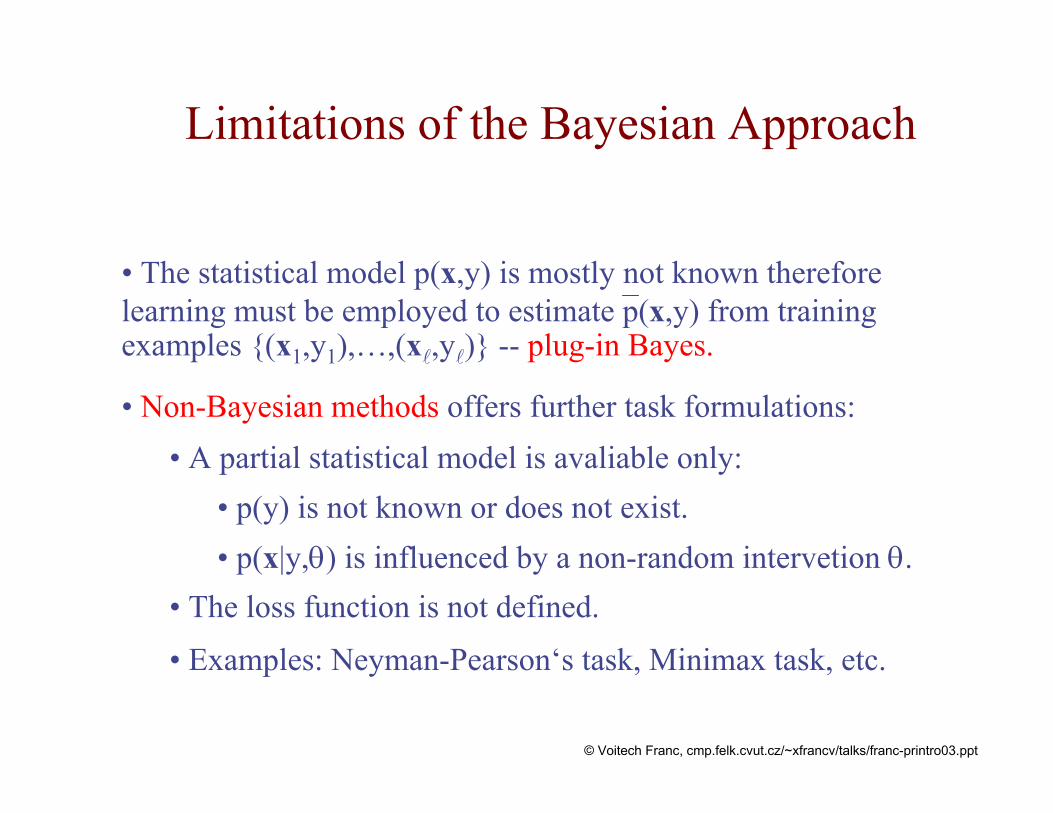
Limitations of the Bayesian Approach
• The statistical model p(x,y) is mostly not known therefore learning must be employed to estimate p(x,y) from training examples {(x1,y1),…,(x ,y )} -- plug-in Bayes.
• Non-Bayesian methods offers further task formulations:• A partial statistical model is avaliable only:
• p(y) is not known or does not exist.• p(x|y,θ) is influenced by a non-random intervetion θ.
• The loss function is not defined.
• Examples: Neyman-Pearson‘s task, Minimax task, etc.
© Voitech Franc, cmp.felk.cvut.cz/~xfrancv/talks/franc-printro03.ppt

Discriminative Approaches
Given a class of classification rules q(x;θ) parametrized by θ∈Ξthe task is to find the “best” parameter θ* based on a set of training examples {(x1,y1),…,(x ,y )} -- supervised learning.
The task of learning: recognition which classification rule is to be used.
The way how to perform the learning is determined by a selected inductive principle.
© Voitech Franc, cmp.felk.cvut.cz/~xfrancv/talks/franc-printro03.ppt

Empirical Risk Minimization Principle
The true expected risk R(q) is approximated by empirical risk
∑=
=1
emp )),;W(q(1));(q(Ri
ii yx θxθ
with respect to a given labeled training set {(x1,y1),…,(x ,y )}.
The learning based on the empirical minimization principle is defined as
));(q(Rminarg emp* θxθ
θ=
Examples of algorithms: Perceptron, Back-propagation, etc.
© Voitech Franc, cmp.felk.cvut.cz/~xfrancv/talks/franc-printro03.ppt

Overfitting and Underfitting
Problem: how rich class of classifications q(x;θ) to use.
underfitting overfittinggood fit
Problem of generalization: a small emprical risk Remp does not imply small true expected risk R.
© Voitech Franc, cmp.felk.cvut.cz/~xfrancv/talks/franc-printro03.ppt

Structural Risk Minimization Principle
An upper bound on the expected risk of a classification rule q∈Q
)1log,,1(R(q)RR(q)σ
hstremp +≤
where is number of training examples, h is VC-dimension of class of functions Q and 1-σ is confidence of the upper bound.
SRM principle: from a given nested function classes Q1,Q2,…,Qm, such that
mhhh ≤≤≤ …21
select a rule q* which minimizes the upper bound on the expected risk.
Statistical learning theory -- Vapnik & Chervonenkis.
© Voitech Franc, cmp.felk.cvut.cz/~xfrancv/talks/franc-printro03.ppt

Unsupervised Learning
Input: training examples {x1,…,x } without information about the hidden state.
Clustering: goal is to find clusters of data sharing similar properties.
Classifier
Learning algorithm
θ
},,{ 1 … xx },,{ 1 … yy
Classifier
ΘY)(X: →×L
YΘX →×:q
Learning algorithm(supervised)
A broad class of unsupervised learning algorithms:
© Voitech Franc, cmp.felk.cvut.cz/~xfrancv/talks/franc-printro03.ppt

Example
k-Means Clustering:
Classifier
1, ,q( ) arg min || ||i
i ky w
== = −x x
…
Goal is to minimize2
q( )1|| ||
iii
w=
−∑ xx
1 ,| |
i
i jji
w∈
= ∑ xII
})q(:{ ij ji == xI
Learning algorithm
1w
2w
3w
},,{ 1 … xx
1{ , , }kw w=θ …
},,{ 1 … yy© Voitech Franc, cmp.felk.cvut.cz/~xfrancv/talks/franc-printro03.ppt

Neural Network References
• Neural Networks, a Comprehensive Foundation, S. Haykin, ed. Prentice Hall (1999)
• Neural Networks for Pattern Recognition, C. M. Bishop, ed Claredon Press, Oxford (1997)
• Self Organizing Maps, T. Kohonen, Springer (2001)
Some ANN Toolboxes• Free software
SNNS: Stuttgarter Neural Network Systems & Java NNSGNG at Uni Bochum
• Matlab toolboxesFuzzy LogicArtificial Neural NetworksSignal Processing

Pattern Recognition / Vector Quantization References
TextbooksDuda, Heart: Pattern Classification and Scene Analysis. J. Wiley & Sons, New York, 1982. (2nd edition 2000).
Fukunaga: Introduction to Statistical Pattern Recognition. Academic Press, 1990.
Bishop: Neural Networks for Pattern Recognition. Claredon Press, Oxford, 1997.
Schlesinger, Hlaváč: Ten lectures on statistical and structural pattern recognition. Kluwer Academic Publisher, 2002.
Related Documents