Lecture 8: Quasi-periodicity, 3-D and higher order sys ...

Lecture notes #8 Nonlinear Dynamics YFX1520

Lecture 8: Quasi-periodicity, 3-D and higher order sys-tems, 3-D limit-cycle, introduction to chaos (determin-istic chaos, chaos theory), chaotic water wheel, Lorenzattractor, coursework requirements

Contents

1 Quasi-periodicity 21.1 Graphical way of thinking about coupled oscillations . . . . . . . . . . . . . . . . . . . . . . 21.2 Example: Decoupled case K1 = K2 = 0 . . . . . . . . . . . . . . . . . . . . . . . . . . . . . 2

1.2.1 Periodic solution for rational slope . . . . . . . . . . . . . . . . . . . . . . . . . . . . 31.2.2 Quasi-periodic solution for irrational slope . . . . . . . . . . . . . . . . . . . . . . . . 4

1.3 Example: Coupled case K1,K2 6= 0 . . . . . . . . . . . . . . . . . . . . . . . . . . . . . . . . 51.3.1 Periodic phase-locked solution, |ω1 − ω2| < K1 +K2 . . . . . . . . . . . . . . . . . . 51.3.2 Quasi-periodic solution with half-stable fixed point, |ω1 − ω2| = K1 +K2 . . . . . . . 61.3.3 Quasi-periodic or periodic solution, |ω1 − ω2| > K1 +K2 . . . . . . . . . . . . . . . . 7

2 3-D systems and introduction to chaos 72.1 Quasi-periodic solution in 3-D systems . . . . . . . . . . . . . . . . . . . . . . . . . . . . . . 72.2 Definition of chaos . . . . . . . . . . . . . . . . . . . . . . . . . . . . . . . . . . . . . . . . . 82.3 Lorenz mill . . . . . . . . . . . . . . . . . . . . . . . . . . . . . . . . . . . . . . . . . . . . . 82.4 Lorenz attractor . . . . . . . . . . . . . . . . . . . . . . . . . . . . . . . . . . . . . . . . . . 10

3 Remark on plotting 3-D phase portraits 11

4 Coursework 124.1 Coursework requirements . . . . . . . . . . . . . . . . . . . . . . . . . . . . . . . . . . . . . . 124.2 Coursework analysis tools . . . . . . . . . . . . . . . . . . . . . . . . . . . . . . . . . . . . . 13

Handout: Coursework requirementsMaterial teaching aids: Trefoil knot, cinquefoil knot

D.Kartofelev 1/13 K As of April 26, 2021


1 Quasi-periodicity

1.1 Graphical way of thinking about coupled oscillations

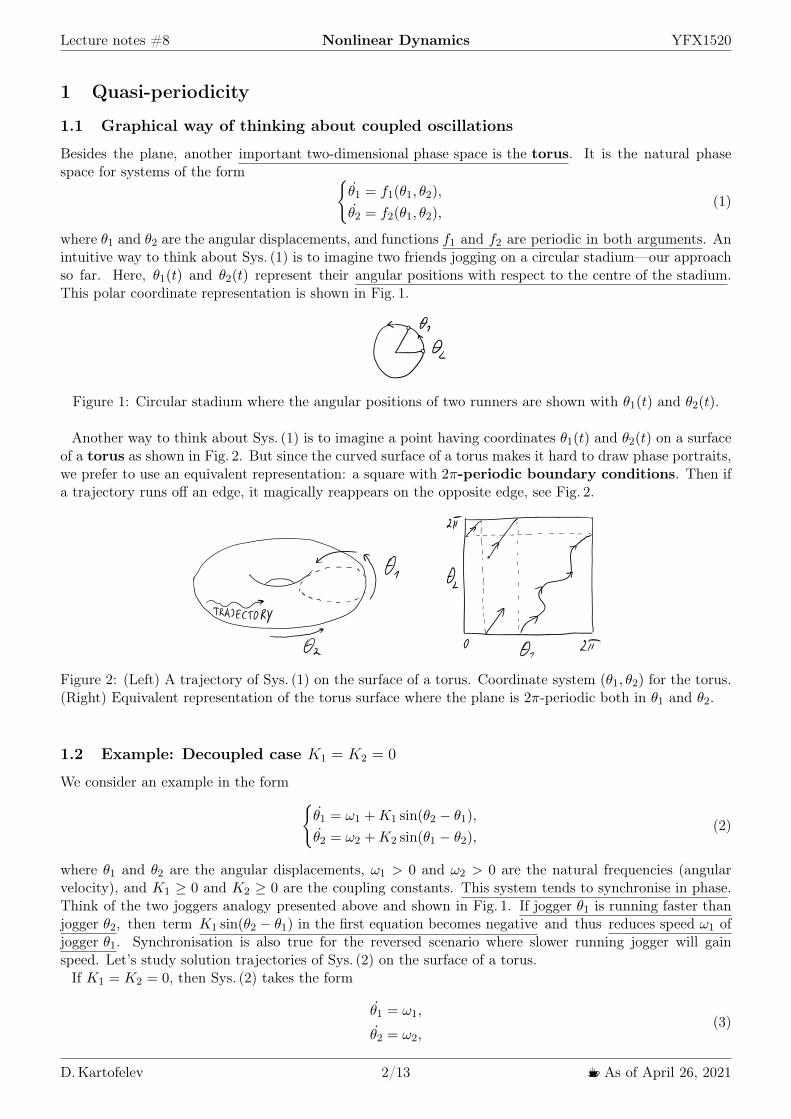
Besides the plane, another important two-dimensional phase space is the torus. It is the natural phasespace for systems of the form {

θ1 = f1(θ1, θ2),

θ2 = f2(θ1, θ2),(1)

where θ1 and θ2 are the angular displacements, and functions f1 and f2 are periodic in both arguments. Anintuitive way to think about Sys. (1) is to imagine two friends jogging on a circular stadium—our approachso far. Here, θ1(t) and θ2(t) represent their angular positions with respect to the centre of the stadium.This polar coordinate representation is shown in Fig. 1.

a

it

II.i

iit I

Figure 1: Circular stadium where the angular positions of two runners are shown with θ1(t) and θ2(t).

Another way to think about Sys. (1) is to imagine a point having coordinates θ1(t) and θ2(t) on a surfaceof a torus as shown in Fig. 2. But since the curved surface of a torus makes it hard to draw phase portraits,we prefer to use an equivalent representation: a square with 2π-periodic boundary conditions. Then ifa trajectory runs off an edge, it magically reappears on the opposite edge, see Fig. 2.

i iI

itItii iiO 21T

0

to I

Figure 2: (Left) A trajectory of Sys. (1) on the surface of a torus. Coordinate system (θ1, θ2) for the torus.(Right) Equivalent representation of the torus surface where the plane is 2π-periodic both in θ1 and θ2.

1.2 Example: Decoupled case K1 = K2 = 0

We consider an example in the form{θ1 = ω1 +K1 sin(θ2 − θ1),θ2 = ω2 +K2 sin(θ1 − θ2),

(2)

where θ1 and θ2 are the angular displacements, ω1 > 0 and ω2 > 0 are the natural frequencies (angularvelocity), and K1 ≥ 0 and K2 ≥ 0 are the coupling constants. This system tends to synchronise in phase.Think of the two joggers analogy presented above and shown in Fig. 1. If jogger θ1 is running faster thanjogger θ2, then term K1 sin(θ2 − θ1) in the first equation becomes negative and thus reduces speed ω1 ofjogger θ1. Synchronisation is also true for the reversed scenario where slower running jogger will gainspeed. Let’s study solution trajectories of Sys. (2) on the surface of a torus.If K1 = K2 = 0, then Sys. (2) takes the form

θ1 = ω1,

θ2 = ω2,(3)



and we are left with a decoupled system. The solution to Sys. (3) is obtained by integrating the relevantequations ∫

θ1dt =

∫ω1dt,

∫θ2dt =

∫ω2dt,

(4)

since ω1 and ω2 are constantθ1(t) = ω1t+ C1,

θ2(t) = ω2t+ C2.(5)

Integration constants can be resolved on the boundary C1 = C2 = 0. The solution trajectories on the 2π-periodic square for any initial condition are straight lines with constant slope dθ2/dθ1 = ω2/ω1. There aretwo qualitatively different cases, depending on whether the slope is a rational or an irrational number.

1.2.1 Periodic solution for rational slope

If the slope is rational, then ω1/ω2 = p/q ∈ Q for some integers p, q ∈ Z (with no common factors). Inthis case all trajectories are closed orbits on the torus, because θ1 completes p revolutions in the same timethat θ1 completes q revolutions. For example, Fig. 3 shows a trajectory on a 2π-periodic square with p = 3and q = 2. When plotted on a torus (in three dimensions), the same trajectory gives a trefoil knot. Allco-prime1 p, q pairs produce knotted trajectories called the toroidal knots, cf. to case p = 10, q = 2 whichproduces a closed spiralling trajectory similar to a closed spring (not a knot). Closed trajectory for p = 5and q = 2 is called cinquefoil knot (also called pentafoil knot, the surgeon’s knot or the Solomon’s sealknot). Slide 4 shows a trefoil knot and a cinquefoil knot as they appear on a torus.

a

it

II.i

iit I

Figure 3: Trefoil knot where p = 3 and q = 2 shown on the 2π-periodic square.

The following numerical file visualises closed trajectories as they appear on the surface of torus for rationalslopes ω1/ω2.

Numerics: nb#1Trajectories on the surface of a torus, interactive 3-D plot. Periodic and quasi-periodic trajectories onthe surface of a torus. Trefoil knot (for p = 3, q = 2). Cinquefoil knot (for p = 5 and q = 2).

The following numerical file shows numerical solution to decoupled Sys. (3) and its phase portrait.

Numerics: nb#2Quasi-periodic oscillators. Quasi-periodic decoupled system: periodic solution, quasi-periodic solution.Fourier and power spectra of the solutions.

1Two integers p and q are said to be relatively prime, mutually prime, or co-prime if the only positive integer (factor) thatdivides both of them is 1.


https://www.ioc.ee/~dima/mittelindyn/numerics_9.nb

https://www.ioc.ee/~dima/mittelindyn/numerics_9b.nb


Slide: 4

Quasi-periodicity2

Transitioning from 2-D to 3-D systems.

Figure: Closed trajectory of Sys. (1) on the surface of a torus. (Left:)Trefoil knot (p = 3, q = 2). (Right:) Cinquefoil knot (p = 5, q = 2).

2See Mathematica .nb file uploaded to course website.D.Kartofelev YFX1520 4 / 19

1.2.2 Quasi-periodic solution for irrational slope

If the slope is irrational ω1/ω2 ∈ P, then the solution is said to be quasi-periodic. In this case trajectorieswill never close into themselves for t→∞. This implies that time-domain solution will never repeat itself.Figure 4 shows this scenario. How can we be sure that trajectories will never close? Any closed trajectorynecessarily makes an integer number of revolutions in both θ1 and θ2; hence the slope would have to berational, contrary to assumption. Furthermore, when the slope is irrational, each trajectory is dense fort� 1 on the torus: in other words, each trajectory comes arbitrarily close to any given point on the torus.This is not to say that the trajectory passes through each point; it just comes arbitrarily close.

a

it

II.i

iit I

Figure 4: A trajectory with irrational slope shown on the 2π-periodic square. The trajectory is not closinginto itself for t→∞.

Quasi-periodicity is significant because it is a new type of long-term behaviour. Unlike the earlierentries: fixed point, closed orbit, cycles, homoclinic and heteroclinic orbits; quasi-periodicity occurs onlyon a torus—a three-dimensional object.The following numerical files shows the numerical solution to decoupled Sys. (3) with its phase portrait

and the dense trajectory of the quasi-periodic solution for irrational slope ω1/ω2 in three-dimensions, re-spectively.

Numerics: nb#2Quasi-periodic oscillators. Quasi-periodic decoupled system: periodic solution, quasi-periodic solution.Fourier and power spectra of the solutions.


https://www.ioc.ee/~dima/mittelindyn/numerics_9b.nb


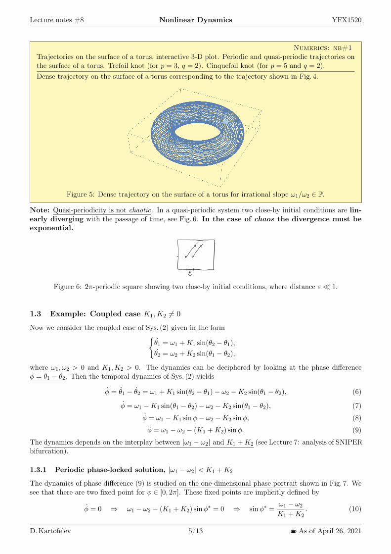
Numerics: nb#1Trajectories on the surface of a torus, interactive 3-D plot. Periodic and quasi-periodic trajectories onthe surface of a torus. Trefoil knot (for p = 3, q = 2). Cinquefoil knot (for p = 5 and q = 2).Dense trajectory on the surface of a torus corresponding to the trajectory shown in Fig. 4.

Figure 5: Dense trajectory on the surface of a torus for irrational slope ω1/ω2 ∈ P.

Note: Quasi-periodicity is not chaotic. In a quasi-periodic system two close-by initial conditions are lin-early diverging with the passage of time, see Fig. 6. In the case of chaos the divergence must beexponential.

a

it

II.i

iit I

Figure 6: 2π-periodic square showing two close-by initial conditions, where distance ε� 1.

1.3 Example: Coupled case K1, K2 6= 0

Now we consider the coupled case of Sys. (2) given in the form{θ1 = ω1 +K1 sin(θ2 − θ1),θ2 = ω2 +K2 sin(θ1 − θ2),

where ω1, ω2 > 0 and K1,K2 > 0. The dynamics can be deciphered by looking at the phase differenceφ = θ1 − θ2. Then the temporal dynamics of Sys. (2) yields

φ = θ1 − θ2 = ω1 +K1 sin(θ2 − θ1)− ω2 −K2 sin(θ1 − θ2), (6)

φ = ω1 −K1 sin(θ1 − θ2)− ω2 −K2 sin(θ1 − θ2), (7)

φ = ω1 −K1 sinφ− ω2 −K2 sinφ, (8)

φ = ω1 − ω2 − (K1 +K2) sinφ. (9)

The dynamics depends on the interplay between |ω1 − ω2| and K1 +K2 (see Lecture 7: analysis of SNIPERbifurcation).

1.3.1 Periodic phase-locked solution, |ω1 − ω2| < K1 +K2

The dynamics of phase difference (9) is studied on the one-dimensional phase portrait shown in Fig. 7. Wesee that there are two fixed point for φ ∈ [0, 2π]. These fixed points are implicitly defined by

φ = 0 ⇒ ω1 − ω2 − (K1 +K2) sinφ∗ = 0 ⇒ sinφ∗ =

ω1 − ω2

K1 +K2. (10)


https://www.ioc.ee/~dima/mittelindyn/numerics_9.nb


I

V

o O 21T

k2

i

it Ii

Figure 7: (Left) One-dimensional phase portrait of phase difference φ where all trajectories are approachingthe stable fixed point. (Right) 2π-periodic square showing stable (solid bold line) and unstable (dashedbold line) non-isolated fixed points (or trajectories on a torus) corresponding to fixed points (10) shown onthe left. The slope of stable and unstable locked solutions is 1, since ω∗ = θ1 = θ2.

As Fig. 7 shows, all trajectories of Sys. (9) approach asymptotically the stable fixed point. Therefore, backon the torus, the trajectories of Sys. (2) approach a stable phase-locked solution in which the oscillatorsare separated by a constant phase difference φ∗. The phase-locked solution is periodic for t� 1; in fact,both oscillators run at the constant frequency given by ω∗ = θ1 = θ2 = ω2 + K2 sinφ

∗. Substituting forsinφ∗, using (10), yields

ω∗ = ω2 +K2ω1 − ω2

K1 +K2⇒ ω∗ =

K1ω2 −K2ω1

K1 +K2. (11)

This frequency is called the compromise frequency because it lies between the natural frequencies of thetwo oscillators. The compromise is not generally halfway; instead the frequencies are shifted by an amountproportional to the coupling strengths K1 and K2, as shown by identity (11). From three-dimensional pointof view stable trajectory ω∗ acts like a 3-D limit-cycle for all initial conditions starting on the surface ofthis torus. The following numerical file shows numerical solution to coupled Sys. (2) and its phase portrait.

Numerics: nb#3Quasi-periodic coupled oscillations. Fourier and power spectra of the solutions.

t

u

Off

IT

Figure 8: (Left) One-dimensional phase portrait of phase difference φ featuring half-stable fixed point.(Middle) Bifurcation diagram where bifurcation point (K1 +K2)

∗ = |ω1 − ω2|. (Right) 2π-periodic squareshowing half-stable (bold line) non-isolated fixed point (or trajectory on a torus) corresponding to the fixedpoints shown on the left.

1.3.2 Quasi-periodic solution with half-stable fixed point, |ω1 − ω2| = K1 +K2

If we pull the natural frequencies apart, say by detuning one of the oscillators, then the locked solutionsapproach each other and coalesce when |ω1 − ω2| = K1 +K2, see Fig. 8 (Right). Thus the locked solutionis destroyed in a saddle-node coalescence of cycles bifurcation. Figure 8 (Left) shows the one-dimensional phase portrait of phase difference φ for the current case. Figure 8 (Middle) shows the saddle-node bifurcation diagram which corresponds to the saddle-node coalescence of cycles bifurcation taking


https://www.ioc.ee/~dima/mittelindyn/numerics_9c.nb


place on the torus. The following numerical file shows numerical solution to coupled Sys. (2) and its phaseportrait.


I

V

o O 21T

k2

i

it IiFigure 9: (Left) One-dimensional phase portrait of phase difference φ. (Right) Flow on the 2π-periodicsquare corresponding to the phase portrait shown on the left.

1.3.3 Quasi-periodic or periodic solution, |ω1 − ω2| > K1 +K2

After the bifurcation, the flow is like that in the decoupled case studied earlier: we have either a quasi-pe-riodic (ω1/ω2 ∈ P) or a rational periodic flow (ω1/ω2 ∈ Q), depending on the parameters. The onlydifference is that now the trajectories on the 2π-periodic square are curvy, not straight. Figure 9 showsthe dynamics corresponding to this case. The following numerical file shows numerical solution to coupledSys. (2) and its phase portrait.


An interactive overview program code for all possible behaviours of Sys. (2) is linked below.

Numerics: nb#4Quasi-periodic coupled oscillations. Interactive code.

2 3-D systems and introduction to chaos

The general form of three-dimensional or third order homogeneous systems is the following

x = f1(x, y, z),

y = f2(x, y, z),

z = f3(x, y, z),

(12)

where f1, f2, and f3 are the given functions. Fixed point/s (x∗, y∗, z∗) of the above system is/are definedby

x = 0

y = 0

z = 0

⇒

f1(x∗, y∗, z∗) = 0,

f2(x∗, y∗, z∗) = 0,

f3(x∗, y∗, z∗) = 0.

(13)

Phase portrait and solution trajectories of a 3-D system are now visualised in three dimensions, see Sec. 3and Slides 16, 17.

2.1 Quasi-periodic solution in 3-D systems

Note: If you see trajectories of a three-dimensional system ending up on the surface of a torus, then thereis a possibility of quasi-periodic solution existing for that system.




https://www.ioc.ee/~dima/mittelindyn/numerics_9d.nb


2.2 Definition of chaos

There is no rigorous mathematical definition of chaos. This shouldn’t defer us from trying. In the nextweek’s lecture we will give a more detailed conceptual definition of chaos in addition to the informationshown below.

Slides: 5–8What happens if you google “chaos”?

Chaos, dictionary definition

Chaos3 in day-to-day laymen jargon (colloquial meaning):

a state of utter confusion or disorder.

a total lack of organisation or order.

complete confusion and disorder; a state in which behaviour andevents are not controlled by anything.

a state of things in which chance is supreme; especially, theconfused unorganised state of primordial matter before thecreation of distinct forms.

any confused, disorderly mass: a chaos of meaningless phrases.

3Source: various online dictionaries.D.Kartofelev YFX1520 5 / 19

Chaos in mathematics and physics

Chaos theory is the field of study in mathematics that studies thebehaviour of dynamical systems that are highly sensitive to initialconditions – a response popularly referred to as the “butterflyeffect”. Small differences in initial conditions (such as those due torounding errors in numerical computation or measurementuncertainty) yield widely diverging outcomes for such dynamicalsystems, rendering long-term prediction impossible in general. Thishappens even though these systems are deterministic, meaning thattheir future behaviour is fully determined by their initial conditions,with no random (stochastic) elements involved. In other words, thedeterministic nature of these systems does not make thempredictable. This behaviour is known as deterministic chaos, orsimply chaos. Chaotic behaviour exists in many natural systems,such as weather and climate. It also occurs spontaneously in somesystems with artificial components, such as road traffic.

D.Kartofelev YFX1520 6 / 19


The fact that deterministic system is not predictable (determined) inpractice is not an internally contradicting statement, its amanifestation of a new mathematical property or type ofsolution of higher order (order more than two) nonlinear systems,called chaos. Also, this long-term aperiodic solution is qualitativelydifferent from the periodic and quasi-periodic solutions since solutionswith slightly different initial conditions deviate exponentially.

The chaos was summarised by Edward Lorenz as:Chaos – when the present determines the future, but the approximatepresent does not approximately determine the future.

When predicting distant future states of a chaotic system one cannever know the starting point accurately enough.



SRB measure (Sinai-Ruelle-Bowen measure) – If statistics oftrajectories of a system are insensitive to initial conditions or smalldifferences of initial conditions then we say that the system has aSRB measure.


The confusing terms “chaos” and “chaos theory” are not useful nor even needed, since as mentionedabove, there are no agreed upon definition of chaos. All aspects of nonlinear and chaotic dynamicalsystems studied in future lectures can be characterised without using the terms “chaos” or “chaotic”—wehave more accurately descriptive and precise terminology.

2.3 Lorenz mill

We begin our study of chaos with a classical example—the Lorenz mill. The simplest version is a toywaterwheel with leaky paper cups suspended from its rim. Water is poured in steadily from the top. If theflow rate is too slow, the top cups never fill up enough to overcome friction, so the wheel remains motionless.For faster inflow, the top cup gets heavy enough to start the wheel turning. Eventually the wheel settlesinto a steady rotation in one direction or the other. By symmetry, rotation in either direction is equallypossible; the outcome depends on the initial conditions.By increasing the flow rate still further, we can destabilise the steady rotation. Then the motion becomes

chaotic: the wheel rotates one way for a few turns, then some of the cups get too full and the wheel doesn’thave enough inertia to carry them over the top, so the wheel slows down and may even reverse its direction.Then it spins the other way for a while. The wheel keeps changing direction erratically. Equations ofmotion of Lorenz mill are shown below.



Slides: 9–11Chaotic systems: Lorenz mill4

Lorenz mill’s or chaotic water wheel’s equations of motion are

a1 = ωb1 −Ka1,

b1 = −ωa1 −Kb1 + q1,

ω = −νIω +

πGr

Ia1,

(2)

where I is the moment of inertia, θ is the angle of the wheel, ω is theangular velocity, K is the liquid’s leakage rate, ν is the damping rate,r is the radius of the wheel, G is the effective gravity constant. a1and b1 are the Fourier amplitudes of the first modes of the liquid’smass distribution function

m(θ, t) =∞∑

n=0

[an(t) sinnθ + bn(t) cosnθ] . (3)


The derivation of equations of motion for this problem is discussed in Chapter 9 of our main textbook.

Chaotic systems: Lorenz mill

g1 is the Fourier amplitude of the first mode of the liquid inflow massdistribution function

Q(θ) =∞∑

n=0

qn cosnθ. (4)

0 10 20 30 40 50

-5

0

5

t

ω(t)

Angular velocity of the wheel


Chaotic systems: Lorenz mill5




Lorenz mill dynamics shows strong dependence on a selection of initial conditions.

Numerical file used to calculate the above results is linked below.

Numerics: nb#5Chaotic system example – Lorenz mill. Power spectrum of Lorenz mill solutions. Numerical solutionplotting in 3-D.Includes a demonstration of system’s sensitive dependence on initial conditions.

Following slides show two video animations of Lorenz mill and its dynamics.

Slides: 12, 13

Chaotic systems: Lorenz mill, chaos

No embedded video files in this pdf


Chaotic systems: Lorenz mill, SRB measure

No embedded video files in this pdf


Some statistical aspects of the rotation might not be sensitive to initial conditions (SRB measure).

2.4 Lorenz attractor

Ed Lorenz derived this three-dimensional system from a drastically simplified model of convection rolls inthe atmosphere. The same equations also arise in simplified models of lasers, dynamos, thermosyphons,brushless DC motors, electric circuits, chemical reactions, forward osmosis, and they exactly describe themotion of Lorenz mill. Lorenz mill is a specific case of Lorenz attractor. The proof can be found in ourmain textbook.

Slides: 14, 15

Chaotic systems: Lorenz attractor

Lorenz attractor:6 It can be shown that Sys. (2) is a specific case ofa more general system in the form

x = σ(y − x),

y = rx− y − xz,

z = xy − bz,

(5)

where σ, r, b > 0 are the control parameters.

Read: E. N. Lorenz, “Deterministic nonperiodic flow”. Journal ofthe Atmospheric Sciences, 20(2), pp. 130–141 (1963).http://dx.doi.org/10.1175/1520-0469(1963)020<0130:

DNF>2.0.CO;2


Chaotic systems: Lorenz attractor


The system has only two nonlinearities, the quadratic terms xy and xz, rendering it a relatively simplechaotic system.

Numerical file linked below contains the time-domain solution of Lorenz attractor.


https://www.ioc.ee/~dima/mittelindyn/numerics_9e.nb


Numerics: nb#6Chaotic system example – Lorenz attractor. Numerical integration of Lorenz attractor (3-D interactive,2-D (x-z projection) interactive).Includes dynamic simulation of trajectory flow.

Reading suggestion

Lorenz’s2 original paper is deep, prescient, and surprisingly readable—look it up!

Link File name CitationPaper#1 paper1.pdf Edward N. Lorenz, “Deterministic nonperiodic flow,” Journal of the Atmo-

spheric Sciences, 20(2), pp. 130–141, (1963).doi:10.1175/1520-0469(1963)020<0130:DNF>2.0.CO;2

3 Remark on plotting 3-D phase portraits

Slides: 16, 17

Remark on 3-D phase portrait visualisation7


Remark on 3-D phase portrait visualisation


Three-dimensional phase portraits are hard to visualise/read using vectors placed into three-dimensionalprojection. Slide 16 shows the vector field of Lorenz attractor in the manner we have been doing itso far for two-dimensional phase portraits, with exception of raising dimensionality by one. A goodgraphical overview can be given by showing a single or couple trajectories as shown on Slide 17. Thisis especially true in the case of chaotic attractors (defined in future lectures).

Numerical file used to calculate the above results is linked below.2Edward N. Lorenz (1917–2008) is often considered to be the discoverer of chaos, this is not true. Chaos was discovered by

Japanese Professor of Electrical Engineering Yoshisuke Ueda (1936-)


https://www.ioc.ee/~dima/mittelindyn/numerics_9f.nb

https://www.ioc.ee/~dima/mittelindyn/paper1.pdf

https://doi.org/10.1175/1520-0469(1963)020%3C0130:DNF%3E2.0.CO;2


Numerics: nb#7Remark on 3-D phase portraits. 3-D phase portrait and flow visualisation of Lorenz attractor.

4 Coursework

The coursework variant3 assigned to you is announced on the course webpage4 (or at TalTech Moodleenvironment). Positively graded coursework is a prerequisite for taking the exam.

4.1 Coursework requirements

The coursework consists of two parts. The first part requires you to analyse a 2-D system and the secondpart requires the analysis of a 3-D system. Completed coursework may be handed over in two parts at anytime during the semester (or before the exam at the latest).

Part 1: Analysis of a 2-D system

1. Perform linear analysis:

• Find a fixed point or points of your system.• Linearise your system about the fixed point or points.• Plot the linearised phase portrait (suggestion).• Determine the type of the linearised fixed point or points.• Determine if/how changes in control parameter values influence the dynamics (type of fixed

point/s) of your system.

2. Perform nonlinear analysis of the full homogeneous system using a computer:

• Compare the type of the nonlinear fixed point or points with the corresponding linearised fixedpoint or points.

• Plot the nonlinear phase portrait. Compare it with the linearised one.• Explain any discrepancy between the nonlinear and linearised systems if any occurs.

3. Perform nonlinear analysis of the non-homogeneous system (if applicable) using a computer:

• Analyse the influence of the explicitly time dependant part of the system on the system dynamics.• Plot the nonlinear non-homogeneous phase portrait. Compare it with the homogeneous one.• Explain the obtained and presented results

4. Draw overall conclusions and comment on the presented results.

Part 2: Analysis of a 3-D system

1. Compare the known properties of strange attractors against your system.

2. Draw conclusions based on your analysis results.

How?

Above problems and specific tasks must be tackled with the use of analysis methods presented and discussedduring the lectures.

Personal consultation

Before submitting the completed and finalised coursework for an evaluation, You have the right to consultthe Lecturer and discuss your progress to ensure that the final submitted coursework is laking any technicalmistakes and/or errors. Please do not hesitate to use this opportunity.

3https://www.ioc.ee/~dima/YFX1520/All_variants.pdf4https://www.ioc.ee/~dima/YFX1520/nimekiri.pdf


https://www.ioc.ee/~dima/mittelindyn/numerics_9g.nb

https://www.ioc.ee/~dima/YFX1520/All_variants.pdf

https://www.ioc.ee/~dima/YFX1520/nimekiri.pdf


4.2 Coursework analysis tools

Students who lack coding skills are welcomed to use the numerical analysis tools provided by the Lecturerand others. These tools don’t require any coding skills—just type in your system and study the resultsdisplayed. For additional information visit the course webpage5.Below are linked the numerical and symbolic analysis tools created specially for this course. The tools

are capable: of performing linear and eigenanalysis of linear and nonlinear systems; to plot 2-D and 3-Dphase portraits; and find/plot numerically integrated time-domain solutions.

Numerics: nb#8Coursework analysis tools: Analysis tool for performing linear analysis of 2-D nonlinear systems,plotting and visualisation of 2-D and 3-D nonlinear systems (Wolfram Mathematica notebook).Requires Wolfram Mathematica installation. Wolfram Player can’t handle it. No coding skills required.

Revision questions

1. What is quasi-periodicity?2. Can quasi-periodic system generate chaotic solution? Why?3. Do limit-cycles exist in 3-D phase spaces? Sketch an example.4. What are 3-D and higher order systems?5. What is chaos in the context of dynamical systems (deterministic chaos, chaos theory)?6. Name properties of chaotic systems.7. What does it mean that a chaotic system has SRB measure (Sinai-Ruelle-Bowen measure)?8. What is chaotic water wheel?9. What is Lorenz attractor?

5https://www.ioc.ee/~dima/YFX1520.html


https://www.ioc.ee/~dima/mittelindyn/Analysis_tool.nb

https://www.ioc.ee/~dima/YFX1520.html

Lecture 8: Quasi-periodicity, 3-D and higher order sys ...

Documents