Lecture #7

Lecture #7

Estimation and Orders of Magnitude

Estimation

Orders of Magnitude

• Powers of 10: http://micro.magnet.fsu.edu/primer/java/scienceopticsu/powersof10/

• Cell size and scale:http://learn.genetics.utah.edu/content/begin/cells/scale/

Content1. Some Overall Observations

2. Metabolism

I. What are Typical Concentrations?

II. What are Typical Metabolic Fluxes?

III. What are Typical Turnover Times?

IV. What are Typical Power Densities?

3. Macromolecules

I. What are Typical Characteristics of a Genome?

II. What are Typical Protein Concentrations?

III. What are Typical Fluxes?

IV. What are Typical Turnover Times?

4. Cell Growth and Phenotypic Functions

5. Summary

Key Concepts

• Characteristic orders of magnitude for key quantities that characterize cellular functions can be estimated

• Data on cell size, mass, composition, metabolic complexity, and genetic makeup are available

• Numerous databases now available on the web • Useful estimates of fluxes, concentrations,

kinetics, and power densities in the intracellular environment can be made based on this data

Enrico Fermi (1901 - 1954) was an Italian physicist, particularly remembered for his work on the development of the first nuclear reactor, and for his contributions to the development of quantum theory, nuclear and particle physics, and statistical mechanics.

Famous for quick answers through back-of-the-envelope calculations

Introduction to Fermi problems

• The classic Fermi problem is:"How many piano tuners are there in Chicago?"

One approximation…• Thzere are approximately 5,000,000 people living in Chicago.• On average, there are two persons in each household in Chicago.• Roughly one household in twenty has a piano that is tuned regularly.• Pianos that are tuned regularly are tuned on average about once per year.• It takes a piano tuner about two hours to tune a piano, including travel time.• Each piano tuner works eight hours in a day, five days in a week, and 50 weeks

in a year.• From these assumptions we can compute that the number of piano tunings in a

single year in Chicago is• (5,000,000 persons in Chicago) / (2 persons/household) × (1 piano/20

households) × (1 piano tuning per piano per year) = 125,000 piano tunings per year in Chicago. We can similarly calculate that the average piano tuner performs

• (50 weeks/year)×(5 days/week)×(8 hours/day)/(1 piano tuning per 2 hours per piano tuner) = 1000 piano tunings per year per piano tuner. Dividing gives

• (125,000 piano tuning per year in Chicago) / (1000 piano tunings per year per piano tuner) = 125 piano tuners in Chicago.

Real significance …

• Possible to estimate key biological quantities on the basis of a few foundational facts and simple ideas from physics and chemistry.

• Numbers collected by the scientific community that initially appear unrelated are brought together as a tool of inference to shed light on biological mechanisms.

Biological examples

• How many proteins can be produced from a single mRNA in E. coli?

• How many ATP synthase complexes are required for optimal growth on glucose in E. coli?

proteins/mRNA: method 1• RNA nucleotide residues / cell: 7.3*107

• Amino acid residues / cell: 8.7*108 – Source: Neidhardt (Vol. 2/Table 2/pg. 1556)

• Fraction of RNA that is mRNA: 0.03 – 0.05 – Source: PMID 11713332

• Total mRNA nucleotide residues: 2,190,000 – 3,650,000 nt

• Average length of mRNA: 1,100 nt• Number of mRNA / cell: 2000-3300• Average length of protein: 367 AA• Number of proteins / cell: 2.4 million• 725-1200 proteins / mRNA:

proteins/mRNA: method 2• Average length of mRNA: 1,100 nt• A ribosome can bind every: 50 nt (structural

consideration)• Maximum ribosome loading: 22 ribosomes/transcript• Rate of translation: 16 AA / sec• All ribosomes working together: 352 AA / sec• Average length of protein: 367 AA• Effective translation speed: About 1 protein/sec• Average half-life of mRNA: 6 minutes (360 seconds)• Mean lifetime of mRNA = 519 seconds (half-life / ln2)• 519 proteins/mRNA

Let’s see how we did…Biological significance:• Many expressed

genes in bacteria are transcribed only once per cell cycle

• Some cells fail to produce an essential message during a cycle, and so must depend on existing messages and/or proteins for survival

Marcotte et al., NBT 2007

Another example: ATP synthase• Motivation: membrane proteins notoriously difficult to quantify• Maximum velocity of ATP synthase: 230 revolutions / sec

(828,000 / hr) [PMID 15668386]• 3 ATP produced / revolution• 2.5 million ATP / hr synthase• Modeled flux required through ATP synthase: 52.0479

mmol/gDwh– Input: Aerobic + 10 mmol glucose / gDwh

• With 2.8*10-13 gDw/cell, and using Avogadro’s number Need 8,773,194,024 ATP / hr to grow optimally [growth rate of 0.7367 doublings/hr or a doubling time of about 1 hr]

• Need 3509 ATP synthase complexes working at Vmax• Number of inner membrane proteins is 200,000• Each ATP synthase complex has 22 proteins• ATP synthase takes accounts for 40% of inner membrane

proteins (constraint for a future genome-scale model?)

Resource: BioNumbers database

Source: http://bionumbers.hms.harvard.edu/BioNumbers is coordinated and developed by Ron Milo at the Weizmann Institute in Israel.

Species # BioNumbersE. coli 920

H. sapiens 667S. cerevisiae 394

SOME OVERALL OBSERVATIONSOrders of Magnitude

The Interior of a Cell:a crowded place

Courtesy of David Goodsellhttp://mgl.scripps.edu/people/goodsell/

The Cellular Environment:highly organized in space (and time)

Typical Cellular Composition

Cellular Composition: historic E. coli data

Representative Time Scales

Multi-scale relationships:

metabolism, transcription, translation, phenotypes

METABOLISMSmall molecule scale

WHAT ARE TYPICAL METABOLITE CONCENTRATIONS?

The compounds

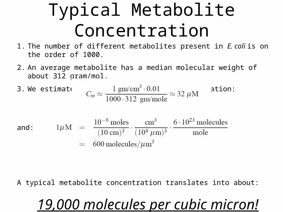
1. The number of different metabolites present in E. coli is on the order of 1000.

2. An average metabolite has a median molecular weight of about 312 gram/mol.

3. We estimate the typical metabolite concentration:

and:

A typical metabolite concentration translates into about:

19,000 molecules per cubic micron!

Typical Metabolite Concentration

Intracellular metabolite concentrations in glucose-fed, exponentially growing E. coli

Rabinowitz et al. Nature Chemical Biology (2009)

Intracellular metabolite concentrations in glucose-fed, exponentially growing E. coli

Rabinowitz et al.Nature Chemical Biology (2009)

Size Distribution of Metabolites

Publicly Available Metabolic Resources

WHAT ARE TYPICAL METABOLIC FLUXES?

Reaction rates

What are Typical Turnover Times?

1. Rate of diffusion varies with many chemical parameters

2. Estimating maximal reaction rates:

One million molecules per cubic micron (cell) per second!

Reaction versus Diffusion

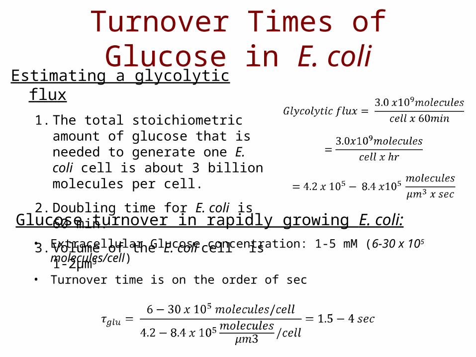
Estimating a glycolytic flux

1. The total stoichiometric amount of glucose that is needed to generate one E. coli cell is about 3 billion molecules per cell.

2. Doubling time for E. coli is 60 min.

3. Volume of the E. coli cell is 1-2µm3

Glucose turnover in rapidly growing E. coli:

• Extracellular Glucose concentration: 1-5 mM (6-30 x 105 molecules/cell)

• Turnover time is on the order of sec

Turnover Times of Glucose in E. coli

Turnover times in RBC glycolysis

Fast and slow:

Distributed time

constants

The Measured Time Response of the Energy Charge

(2ATP+ADP) 2(ATP+ADP+AMP)

TWO FUNDAMENTAL CONTROL/REGULATORY CHALLENGES:

1. “Disturbance rejection” – return to the original state2. “Servo” – transition from one steady state to the other steady state

A bi-phasic response: rapid decay and slow recovery

The rapid response of energy transducing membranes

(Redox Metabolism)

Charge on Energy Transducing Membranes

• Majority of biological energy transducing membranes have potential between -180 and -230 mV

• Bi-lipid layers become physically unstable at -280 mV

Magnitude of the potential gradient

1. As presented above the potential is on the order of -220-240 mV across the energy transducing membrane.

2. The thickness of the lipid bi-layer is on the order of 7nm.

3. So the potential gradient across this membrane is:

• 230 mV/7 nm = 300,000 V/cm

4. A potential gradient of 1,000 V/cm produces a spark in the air (car spark plug).

ESTIMATING THE NUMERICAL VALUE OF KINETIC CONSTANTS

Kinetic Constants of E. coli Enzymes

http://www.brenda-enzymes.info/

32 M32 M • Majority of kinetic information is based on the in vitro measurements – might not be physiologically relevant

•Average Enzyme concentration s on the order of an average kinetic constant (S ~ Km)

Typical Enzyme Turnover Times

http://www.brenda-enzymes.info/

1 min1 min

The Distributions of Gibbs Free Energies in iAF1260

Exothermic Endothermic

WHAT ARE TYPICAL POWER DENSITIES?

1. Power output of rat mitochondria• Typical ATP production in mitochondria is

6 x 10-19 mol ATP/mitochondria/sec.

• Volume of the inner matrix in mitochondria is 0.27 μm3

• The energy of the phosphate bond is about 52 kJ/mol ATP

2. Power output of chloroplast in C. reinhardtii (green algae)• Typical ATP production in chloroplast:

9.0 x 10-17 to 1.4 x 10-16 mol ATP/chloroplast/sec.

• Volume of a chloroplast 17.4 μm3

33133

19

/1.0/101.152

27.0sec

106mpWmW

molATP

kJ

m

iamitochondr

iamitochondr

molATP

33133

1617

/2.0/10252

4.17sec

101109mpWmw

molATP

kJ

m

tchloroplas

tchloroplas

molATP

3. Power production density in a rapidly growing E. coli• ATP production: 0.3 - 2.0 x 10-17 mol ATP/cell/sec

• Volume of E. coli 1 μm3

4. Power production by the sun• Radiant power of the sun 3.86 x 1026 W

• Volume of the sun is 1.4 x 1027 m3

The power density of the sun is six orders of magnitude lower

33133

17

/6.0/10100.252

1sec

100.23.0mpWmW

molATP

kJ

m

cell

cell

molATP

363193327

26

/103.0/107.227.010412.1

1086.3mpWmW

m

W

m

W

Summary: metabolism• Diffusion times are 1-10 msec faster than reactions• Average concentration is about 30 M • Maximal fluxes are about a million molecules per

per sec• Redox pools respond on the order of sec or faster,

energy charge on the order of a min

• Average Km is 32 m close to substrate concentrations

• Enzyme turnover times are < min• Power densities are on the order of 0.1-0.5 pW/3

SYNTHESIS OF MACROMOLECULES: DNA, RNA AND PROTEIN

Macromolecular scale

Characteristics of Genomes

- First sequenced genome (1995)- Smallest free living organism

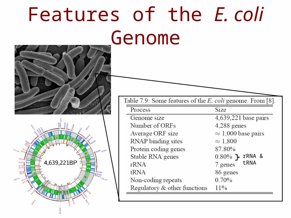
Features of the E. coli Genome

rRNA & tRNA

Features of the Human Genome

Based on NCBI assembly Build 36 (released 2005) (http://www.ensembl.org/Homo_sapiens/index.html)

Topic StatisticTotal size of the genome: approximately 3,200,000,000 bp

Percentage of adenine (A) in the genome: 54%Percentage of cytosine (C) in the genome: 38%

Percentage of bases not yet determined: 9%Highest gene-dense chromosome: chromosome 19 with 23 genes per 1,000,000 bp

Least gene-dense chromosomes: chromosome 13 and Y with 5 genes per 1,000,000 bpPercentage of DNA spanned by genes: between 25% and 38%

Percentage of exons: 1.1 to 1.4%Percentage of introns: 24% to 37%

Percentage of intergenic DNA: 74% to 64%The average size of a gene: 27,000 bp

The longest gene: dystrophin (a muscle protein) with 2,400,000 bpAverage length of an intron: 3,300 bp

Most common length of an intron: 87 bpOccurrence rate of SNPs: roughly 1 per 1,500 bp

SNRs: 12,228,116Occurrence rate of genes: about 12 per 1,000,000 bp

RNA genes: 4,150

WHAT ARE TYPICAL PROTEIN CONCENTRATIONS?

1. Cells represent a fairly dense solutions of proteins

2. Concentration of total protein in cells falls in the range: 200 – 400 mg/ml

3. For E. coli we can assume:

• A cell has 1000 or so different proteins expressed at significant levels

• Average molecular weight of a protein is: 35 kDa.

• Protein is about 15% of wet weight of the cell or about 55% of the dry cell weight

About 2500 molecules of a particular protein molecule per cubic micron!

With 1000 proteins present in the cell the total amount of protein molecules is: 2.5 x 106 proteins/cell

Protein Concentration in E. coli

Size distribution of ORF or Protein sizes in E. coli

Distribution of Protein Concentrations in E. coli

Size distribution of protein concentrations in E. coli K12 MG1655. Panel A: Relative log (base 2) values of protein abundances rank-ordered; Panel B: Relative protein abundance distribution.

Publicly Available Proteomic Resources

WHAT ARE TYPICAL SYNTHETIC FLUXES OF MACROMOLECULES?

Typical Fluxes: DNA synthesis1. The E. coli genome can be replicated in 40 min with 2

replication forks – the rate of DNA polymerase is:

2. The rate of RNA polymerase is much slower:

Process RateDNA Replication (DNA -> DNA) 900 bp/sec/fork

Transcription (DNA -> RNA) 40-50 bp/secTranslation (RNA -> Protein 12-20 amino acids/sec

Protein Synthesis in E. coli1. The rate of the ribosome is on the order of 12-21 peptide

bonds/ribosome/sec in rapidly growing E. coli.

2. The amount of ribosomes present in E. coli depends vastly on the growth rate: on the order of: 7x103 – 7x104 ribosomes/cell

3. The total amount of peptide bonds that are formed in E. coli as a function of growth rate can be estimated:

4. This value is equivalent to:

sec

105.1108107107

sec

2112 6443

cell

pbxx

cell

ribosomesxx

ribosome

pb

hourcell

proteinsx

cell

proteins

61031

sec

900300

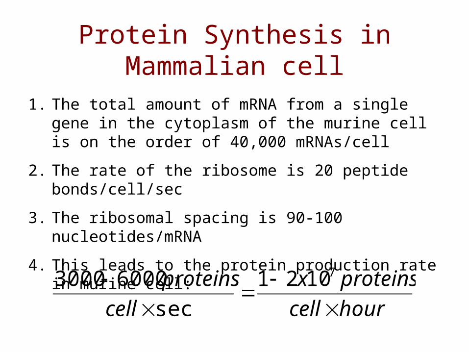
Protein Synthesis in Mammalian cell

1. The total amount of mRNA from a single gene in the cytoplasm of the murine cell is on the order of 40,000 mRNAs/cell

2. The rate of the ribosome is 20 peptide bonds/cell/sec

3. The ribosomal spacing is 90-100 nucleotides/mRNA

4. This leads to the protein production rate in murine cell:

hourcell

proteinsx

cell

proteins

71021

sec

60003000

CELL GROWTH AND PHENOTYPIC FUNCTIONS

The whole-cell scale

Phenotypic characteristics of E. coli: Aerobic (60 min) and Anaerobic profile (90 min)

Flux Nameoxic anoxic oxic anoxic

Glucose Uptake 17.9 +/- 1.2 9.02 +/- 0.23 9.0 x 105 4.50 x 105

Oxygen Uptake 0 14.92+/-0.21 0 7.50 x 105

Formate Secretion 15.8 +/- 1.8 3.51 +/- 0.47 7.90 x 105 1.76 x 105

Acetate Secretion 10.9 +/- 0.8 3.37 +/- 0.02 5.45 x 105 1.70 x 105

Ethanol Secretion 7.4 +/- 0.6 0 3.70 x 105 0

Succinate Secretion 1.1+/- 0.4 0 5.50 x 104 0

Lactate Secretion 0.2 +/- 0.1 0 1.0 x 104 0

Rate (mmol/gDW/h) molecules/µm3/sec

Synthesis of an E. coli Cell: order-of-magnitude estimation of fluxes

• There are 3.0 x106 proteins per cell, each with an average length of 316 AA.

• If the ribosome can make 20 peptide bonds/sec = 1200 pb/min = 72,000 pb/hr:

Nucleotide requirement per hour (or cell division):

for a grand total of approximately 9.26 x 107 nucleotides/cell for synthesis of RNA and DNA

molecules for one cell.

RNA:

DNA:

Stable RNA

mRNA

chromosome

• The glucose uptake has to be balanced for energy production rate (at about 18 ATP/glucose-aerobically and 3 ATP/glucose-anaerobically) and to meet the biosynthetic rates, that will also have to include cell wall and lipid synthesis.

• Thus the energy equivalent produced is:

Synthesis of an E. coli Cell: order-of-magnitude estimation of fluxes (cont)

H+

ATPADP

H+

ATP Production rate:

0.8 - 4 x 1010 molecules/cell/h METABOLISM

Glycolytic flux: 3 x 109 molecules/cell/h

DNA

mRNA

Protein

Amino Acid Flux:

9 x 108 amino acid/cell/h

Ribosome rate: 3 x 109 peptide bonds/cell/h

Protein production rate:

3 x 106 proteins/cell/h

RNA Polymerase rate:

5 x 108 nucleotides/cell/h

Fraction of RNAP synthesizing tRNA/rRNA:

0.28-0.77

tRNA

Cell doubling time:

60 min

-230 mV -> 105 V/cm

DNA replication rate:

900 bp/sec/fork

Energy production: 0.2 – 1.0 pW/µm3

Nucleotide Flux:

5 x 108 nucleotides/cell/h

Overall metabolic rates in E. coli:Implications for bioprocessing

• Reduced by-products are produced anaerobically• Glycolytic flux often is the entry point of the sugar to the metabolism• E. coli is a commonly used for metabolic engineering applications • Successful metabolic engineering design is usually characterized by its volumetric productivity

Flux Name Rate (mmol/gDW/h) molecules/µm3/secGlucose Uptake 17.9 +/- 1.2 2.98E+06

Formate Secretion 15.8 +/- 1.8 2.63E+06Acetate Secretion 10.9 +/- 0.8 1.83E+06Ethanol Secretion 7.4 +/- 0.6 1.25E+06

Succinate Secretion 1.1+/- 0.4 1.83E+05Lactate Secretion 0.2 +/- 0.1 3.33E+04

Limits on Volumetric Productivity• Anaerobically E. coli has substrate uptake rate (SUR) of:

15 – 20 mmol Glucose/ gDW/h

• Which translates to: 1.5 gram Glucose /L/h

• If all the glucose is converted to the desired product (i.e. D-Lactate), the VOLUMETRIC PRODUCTIVITY of this strain design is: ~ 3 gram Lactate/L/h

• Some metabolically engineered E. coli strains have SUR higher then reported above, leading to higher volumetric productivity.

FROM BACTERIA TO MAMMALS

Metabolic rate of major organs

Size range of living organisms

Figure taken: K. Schmidt-Nielsen, “Why is animal size so important”, 1984

Metabolic rate and body size

Figure taken: K. Schmidt-Nielsen, “Why is animal size so important”, 1984

Summary• The size of a bacterial cell is around 1 µm with a weight of 1 pg. • The interior of the cell is a viscous solution crowded with several

molecular species• The cells are mostly composed of water and macromolecules with

simple metabolites forming only a small fraction. • Typical concentrations of metabolites and enzymes within the cell fall

in the micromolar range with a wide distribution around the mean.• Metabolites are present at an average concentration of 19,000

molecules/µm3, while enzymes have an average concentration of 2000 molecules/µm3.

• Diffusional response times for bacteria, on the order of milliseconds, are much faster than the metabolic dynamics. Spatial distributions can therefore be neglected.

• Metabolic fluxes occur at average rates of 104 to 105 molecules/µm3 /sec.

O-OF-MAGNITUDE: some examples

We'll start with a $100 dollar bill.

The magnitude of the bailout package

A packet of one hundred $100 bills is less than 1/2"

thick and contains $10,000.

http://sketchup.google.com/

Believe it or not, this next little pile is $1 million dollars (100 packets of $10,000).

http://sketchup.google.com/

$100 million is a little more respectable. It fits neatly on a standard pallet...

And $1 BILLION dollars... now we're really getting somewhere...

http://sketchup.google.com/

Ladies and gentlemen... I give you $1 trillion dollars...

Next we'll look at ONE TRILLION dollars. This is that number we've been hearing about so much. What is a trillion dollars? Well, it's a million million. It's a thousand billion. It's a one followed by 12 zeros.

So the next time you hear someone toss around the phrase "trillion dollars"... that's what they're talking about.