Lecture 4 Page 1 CS 239, Spring 2007 Models and Linear Regression CS 239 Experimental Methodologies for System Software Peter Reiher April 12, 2007.

Lecture 4Page 1CS 239, Spring 2007

Models and Linear RegressionCS 239

Experimental Methodologies for System Software

Peter ReiherApril 12, 2007


Introduction

• Models


• Often desirable to predict how a system would behave– For situations you didn’t test

• One approach is to build a model of the behavior– Based on situations you did test

• How does one build a proper model?

Modeling Data


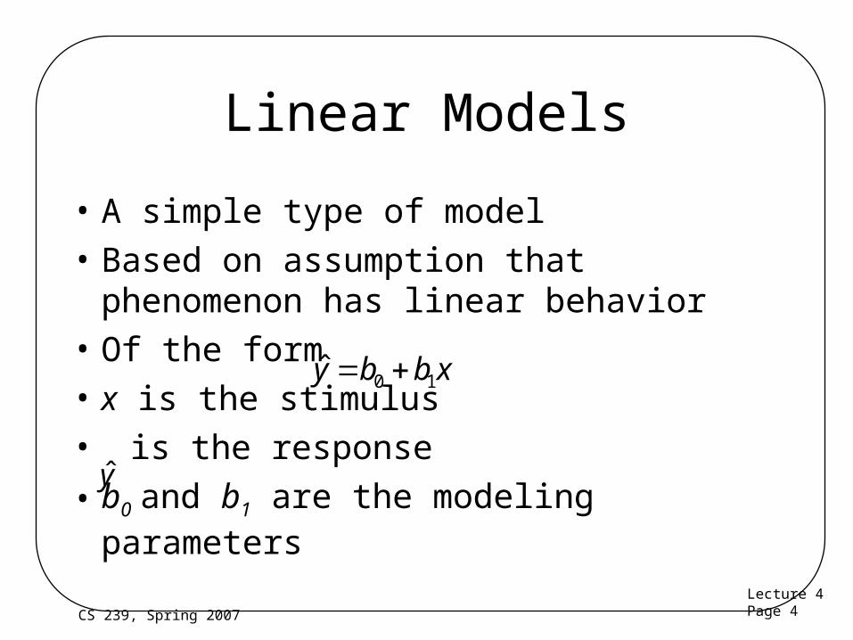
Linear Models

• A simple type of model

• Based on assumption that phenomenon has linear behavior

• Of the form

• x is the stimulus

• is the response

• b0 and b1 are the modeling parameters

xbby 10ˆ

y


Building a Linear Model

• Gather data for some range of x’s

• Use mathematical methods to estimate b0 and b1

– Based on the data gathered

• Analyze resulting model to determine its accuracy


• For correlated data, model predicts response given an input

• Model should be equation that fits data

• Standard definition of “fits” is least-squares

– Minimize squared error

– While keeping mean error zero

– Minimizes variance of errors

Building a Good Linear Model


Least Squared Error

• If then error in estimate for xi

is

• Minimize Sum of Squared Errors (SSE)

• Subject to the constraint

e y yi i i

e y b b xii

n

i ii

n2

10 1

2

1

e y b b xii

n

i ii

n

10 1

1

0

xbby 10ˆ


• Best regression parameters are

where

bxy nxy

x nx1 2 2

b y b x0 1

xn

xi 1 yn

yi 1

xy x yi i x xi2 2

Estimating Model Parameters


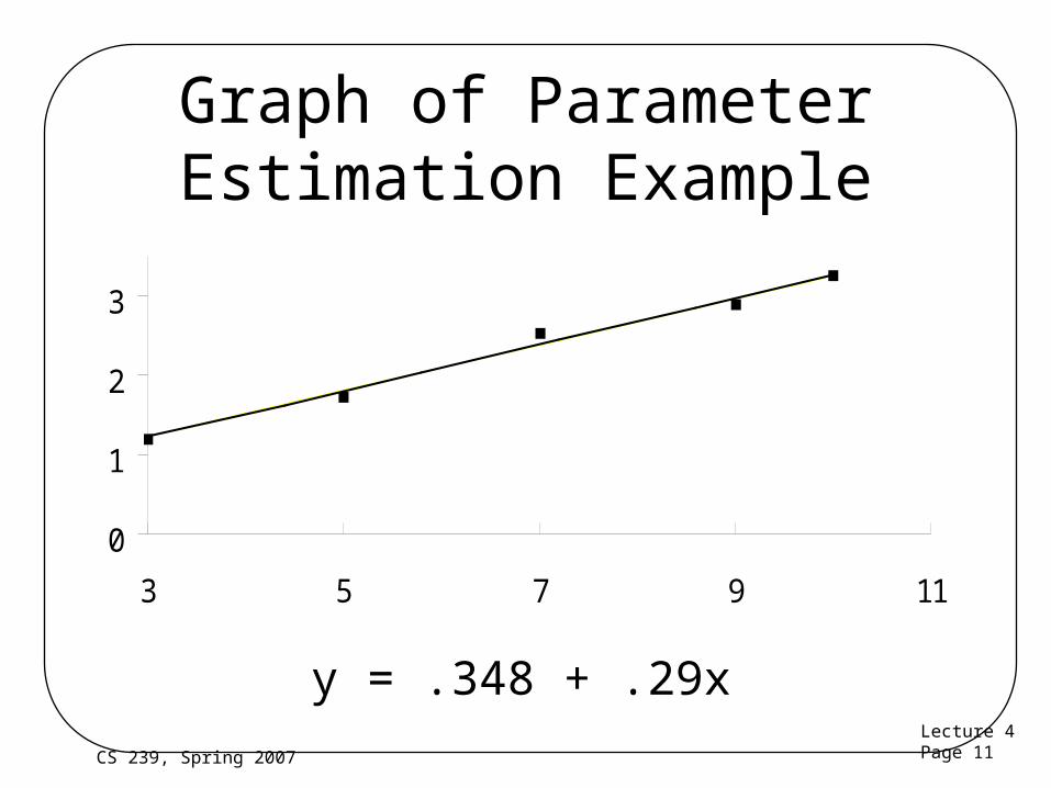
Parameter EstimationExample

• Execution time of a script for various loop counts:

• = 6.8, = 2.32, xy = 88.54, x2 = 264

• b0 = 2.32 (0.29)(6.8) = 0.35

Loops 3 5 7 9 10Time 1.19 1.73 2.53 2.89 3.26

x y


Finding b0 and b1

b1 2

88 54 5 6 8 2 32

264 5 6 80 29

. . .

..b

xy nxy

x nx1 2 2

b y b x0 1 )8.6(*29.32.20 b

= .348


Graph of Parameter Estimation Example

0

1

2

3

3 5 7 9 11

y = .348 + .29x


• If no regression, best guess of y is

• Observed values of y differ from , giving rise to errors (variance)

• Regression gives better guess, but there are still errors

• We can evaluate quality of regression by allocating sources of errors

y

y

Allocating Variation in Regression


The Total Sum of Squares (SST)

• Without regression, squared error is

SST

SSY SS

y y y y y y

y y y ny

y y ny ny

y ny

ii

n

i ii

n

ii

n

ii

n

ii

n

ii

n

2

1

2 2

1

2

1 1

2

2

1

2

2

1

2

2

2

2

0


The Sum of Squaresfrom Regression

• Recall that regression error is SSE =

• Error without regression is SST

• So regression explains SSR = SST - SSE

• Regression quality measured by coefficient of

determinationR2

SSR

SST

SST SSE

SST

e y b b xii

n

i ii

n2

10 1

2

1


Evaluating Coefficientof Determination (R2)

• Compute

• Compute

• Compute

SST ( ) y ny2 2

SSE y b y b xy20 1

R2 SST SSE

SST


Example of Coefficientof Determination

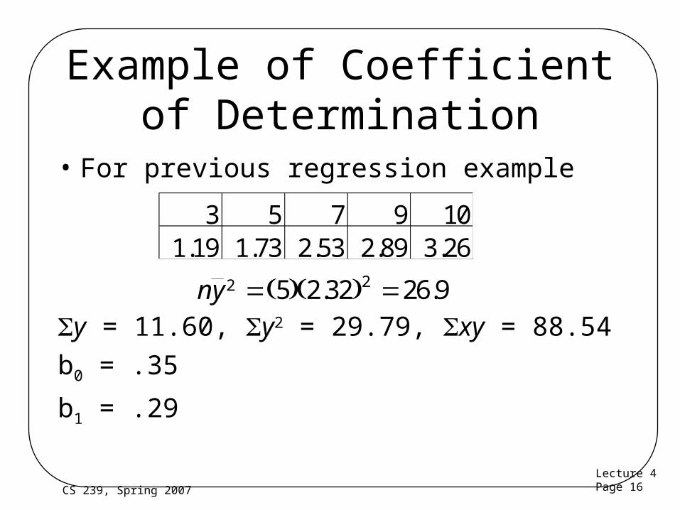
• For previous regression example

y = 11.60, y2 = 29.79, xy = 88.54

b0 = .35

b1 = .29

3 5 7 9 101.19 1.73 2.53 2.89 3.26

ny2 25 2 32 26 9 . .


Continuing the Example

• SSE = - -

• SST = -

• SSR = -

• R2 = /

Σ y2 b0Σ y b1Σ xy29.79 0.35*11.6 0.29*88.54= 0.05

26.9Σ y2 2yn29.79= 2.89

SST SSE 2.89 .05 = 2.84 SSR2.84 SST2.89 = 0.98

• So regression explains most of variation


Standard Deviation of Errors• Variance of errors is SSE divided by

degrees of freedom

– DOF is n2 because we’ve calculated 2 regression parameters from the data

– So variance (mean squared error, MSE) is SSE/(n2)


Stdev of Errors, Con’t

• Standard deviation of errors is square root

of mean squared error:

sne

SSE

2


Checking Degrees of Freedom• Degrees of freedom always equate:

– SS0 has 1 (computed from )

– SST has n1 (computed from data and , which uses up 1)

– SSE has n2 (needs 2 regression parameters)

– So

y

y

SST SSY SS SSR SSE

( )

0

1 1 1 2n n n


Example of Standard Deviation of Errors

• For our regression example, SSE was 0.05,

– MSE is 0.05/3 = 0.017 and se = 0.13

• Note high quality of our regression:

– R2 = 0.98

– se = 0.13

– Why such a nice straight-line fit?


• Regression is done from a single population sample (size n)

– Different sample might give different results

– True model is y = 0 + 1x

– Parameters b0 and b1 are really means taken from a population sample

How Sure Are We of Parameters?


Confidence Intervals of Regression Parameters

• Since b0 and b1 are only samples, • How confident are we that they are

correct?• We express this with confidence

intervals of the regression• Statistical expressions of likely bounds

for true parameters 0 and 1


Calculating Intervalsfor Regression Parameters

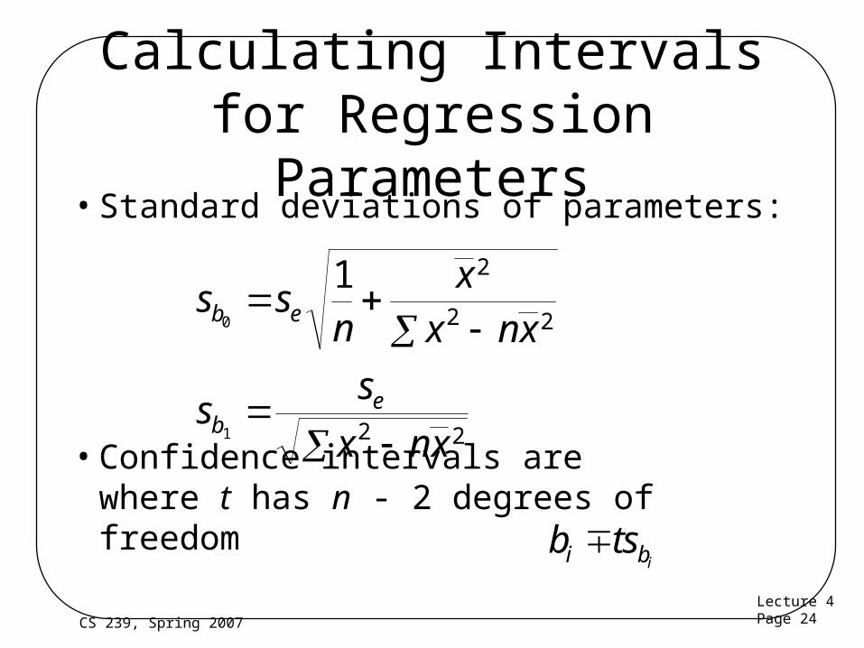
• Standard deviations of parameters:

• Confidence intervals arewhere t has n - 2 degrees of freedom

s sn

x

x nx

ss

x nx

b e

be

0

1

1 2

2 2

2 2

b tsi bi


Example of Regression Confidence Intervals

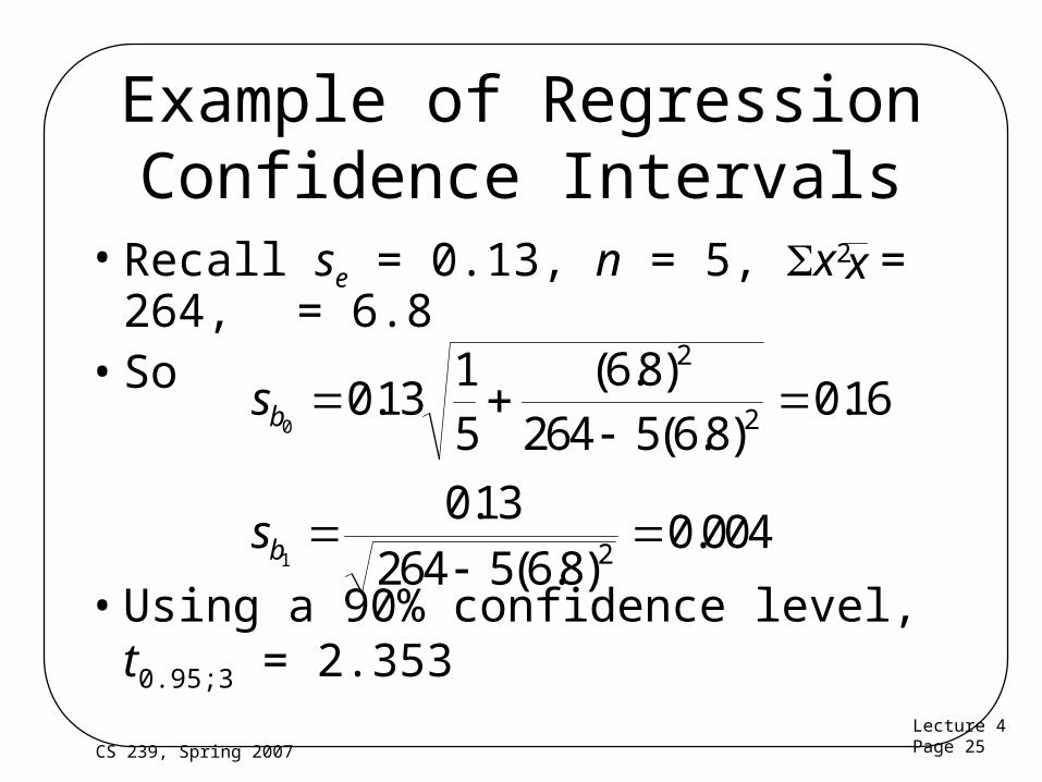
• Recall se = 0.13, n = 5, x2 = 264, = 6.8• So

• Using a 90% confidence level, t0.95;3 = 2.353

x

s

s

b

b

0

1

0 131

5

6 8

264 5 6 80 16

0 13

264 5 6 80 004

2

2

2

.( . )

( . ).

.

( . ).


Regression Confidence Example, cont’d

• Thus, b0 interval is

• And b1 is

0 35 2 353 0 16 0 03 0 73. . ( . ) ( . , . )

0 29 2 353 0 004 0 28 0 30. . ( . ) ( . , . )


Are Regression Parameters Significant?

• Usually the question is “are they significantly different than zero?”

• If not, simpler model by dropping that term• Answered in usual way:

– Does their confidence interval include zero?

– If so, not significantly different than zero• At that level of confidence


Are Example Parameters Significant?

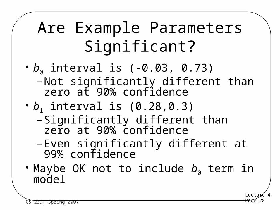
• b0 interval is (-0.03, 0.73)– Not significantly different than zero at

90% confidence• b1 interval is (0.28,0.3)

– Significantly different than zero at 90% confidence

– Even significantly different at 99% confidence

• Maybe OK not to include b0 term in model


Confidence Intervals for Predictions

• Previous confidence intervals are for parameters– How certain can we be that the

parameters are correct?– They say the parameters are likely to

be within a certain range


But What About Predictions?

• Purpose of regression is prediction– To predict system behavior for values we

didn’t test– How accurate are such predictions?– Regression gives mean of predicted

response, based on sample we took• How likely is the true mean of the

predicted response to be that?


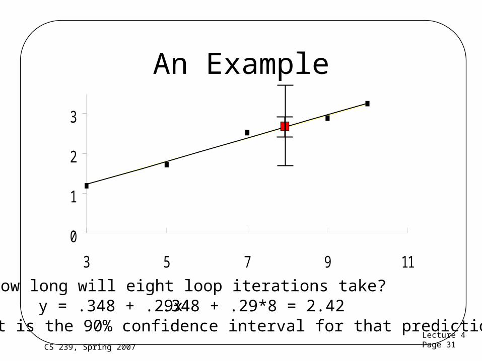
An Example

0

1

2

3

3 5 7 9 11

How long will eight loop iterations take?y = .348 + .29x .348 + .29*8 = 2.42

What is the 90% confidence interval for that prediction?


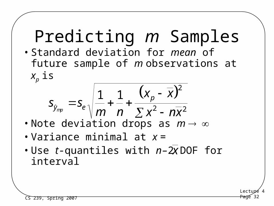
Predicting m Samples• Standard deviation for mean of future

sample of m observations at xp is

• Note deviation drops as m • Variance minimal at x = • Use t-quantiles with n–2 DOF for interval

s s

m n

x x

x nxy ep

mp

1 1

2

2 2

x


Example of Confidenceof Predictions

• Predicted time for single run of 8 loops?

• Time = 0.348 + 0.29(8) = 2.42

• Standard deviation of errors se = 0.13

• 90% interval is then

sy p .

.

( . ).

10 13 1

1

5

8 6 8

264 5 6 80 14

2

)75.3,09.2()14.0(353.242.2


A Few Observations

• If you ran more tests, you’d predict a narrower confidence interval– Due to 1/m term

• Lowest confidence intervals closest to center of measured range– They widen as you get further out– Particularly beyond the range of what

was actually measured


• Regressions are based on assumptions:– Linear relationship between response y and

predictor x– Or nonlinear relationship used to fit– Predictor x nonstochastic and error-free– Model errors statistically independent

• With distribution N(0,c) for constant c• If these assumptions are violated, model misleading

or invalid

Verifying Assumptions Visually


How To Test For Validity?

• Statistical tests are possible

• But visual tests often helpful

– And usually easier

• Basically, plot the data and look for obviously bogus assumptions


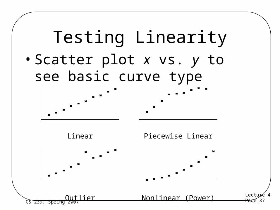
Testing Linearity• Scatter plot x vs. y to see basic curve

type

Linear Piecewise Linear

Outlier Nonlinear (Power)


Testing Independenceof Errors

• Scatter-plot i (errors) versus

• Should be no visible trend

• Example from our curve fit:

yi

-0.1

-0.05

0

0.05

0.1

0.15

0.2

0 0.5 1 1.5 2 2.5 3 3.5 4


More Examples

-1

-0.8

-0.6

-0.4

-0.2

0

0.2

0.4

0.6

0.8

0 2 4 6 8 10 12 14

-0.6

-0.4

-0.2

0

0.2

0.4

0.6

0 2 4 6 8 10 12 14

No obvious trend in errors Errors appear to increase linearly with x valueSuggests errors are not independent for this data set


More on Testing Independence

• May be useful to plot error residuals versus experiment number

– In previous example, this gives same plot except for x scaling

• No foolproof tests

• And not all assumptions easily testable


Testing for Normal Errors

• Prepare quantile-quantile plot

• Example for our regression:

-0.15

-0.1

-0.05

0

0.05

0.1

0.15

0.2

-2.6 -1.3 0 1.3

Since plot is approximately linear, normality assumption looks OK


Testing for Constant Standard Deviation of Errors

• Property of constant standard deviation of errors is called homoscedasticity

– Try saying that three times fast

• Look at previous error independence plot

• Look for trend in spread


Testing in Our Example

-0.1

-0.05

0

0.05

0.1

0.15

0.2

0 0.5 1 1.5 2 2.5 3 3.5 4

No obvious trend in spreadBut we don’t have many points


Another Example

-150

-100

-50

0

50

100

150

0 5 10 15 20 25

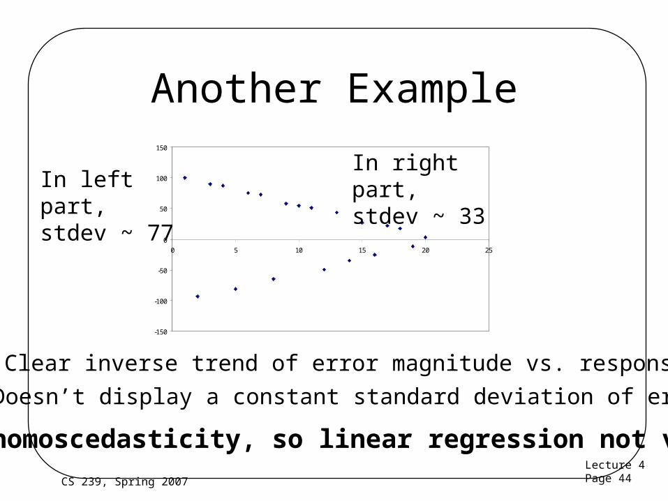
Clear inverse trend of error magnitude vs. response

Doesn’t display a constant standard deviation of errors

In left part, stdev ~ 77

In right part, stdev ~ 33

No homoscedasticity, so linear regression not valid


So What Do You Do With Non-Homoscedastic Data?

• Spread of scatter plot of residual vs. predicted response is not homogeneous

• Then residuals are still functions of the predictor variables

• Transformation of response may solve the problem

• Transformations discussed in detail in book


Is Linear Regression Right For Your Data?

• Only if general trend of data is linear

• What if it isn’t?

• Can try fitting other types of curves instead

• Or can do a transformation to make it closer to linear


Confidence Intervalsfor Nonlinear Regressions

• For nonlinear fits using exponential transformations:

– Confidence intervals apply to transformed parameters

– Not valid to perform inverse transformation on intervals


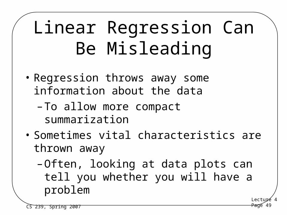
Linear Regression Can Be Misleading

• Regression throws away some information about the data

– To allow more compact summarization

• Sometimes vital characteristics are thrown away

– Often, looking at data plots can tell you whether you will have a problem


Example of Misleading Regression

I II III IV x y x y x y x y 10 8.04 10 9.14 10 7.46 8 6.58 8 6.95 8 8.14 8 6.77 8 5.76 13 7.58 13 8.74 13 12.74 8 7.71 9 8.81 9 8.77 9 7.11 8 8.84 11 8.33 11 9.26 11 7.81 8 8.47 14 9.96 14 8.10 14 8.84 8 7.04 6 7.24 6 6.13 6 6.08 8 5.25 4 4.26 4 3.10 4 5.39 19 12.50 12 10.84 12 9.13 12 8.15 8 5.56 7 4.82 7 7.26 7 6.42 8 7.91 5 5.68 5 4.74 5 5.73 8 6.89


What Does Regression Tell Us About These Data Sets?

• Exactly the same thing for each!• N = 11• Mean of y = 7.5• y = 3 + .5 x• Standard error of regression is 0.118• All the sums of squares are the same• Correlation coefficient = .82• R2 = .67


Now Look at the Data Plots

0

2

4

6

8

10

12

0 5 10 15 200

2

4

6

8

10

12

0 5 10 15 20

0

2

4

6

8

10

12

14

0 2 4 6 8 10 12 14 16

0

2

4

6

8

10

12

14

0 5 10 15 20

I II

III IV


Other Regression Issues

• Multiple linear regression

• Categorical predictors

• Transformations

• Handling outliers

• Common mistakes in regression analysis


Multiple Linear Regression

• Models with more than one predictor variable

• But each predictor variable has a linear relationship to the response variable

• Conceptually, plotting a regression line in n-dimensional space, instead of 2-dimensional


Regression With Categorical Predictors

• Regression methods discussed so far assume numerical variables

• What if some of your variables are categorical in nature?

• Use techniques discussed later in the class if all predictors are categorical

• Levels - number of values a category can take


Handling Categorical Predictors• If only two levels, define bi as follows

– bi = 0 for first value– bi = 1 for second value

• Can use +1 and -1 as values, instead• Need k-1 predictor variables for k levels

– To avoid implying order in categories


Outliers• Atypical observations might be outliers

– Measurements that are not truly characteristic

– By chance, several standard deviations out

– Or mistakes might have been made in measurement

• Which leads to a problem

Do you include outliers in analysis or not?


Handling Outliers

1. Find them (by looking at scatter plot)2. Check carefully for experimental

error3. Repeat experiments at predictor

values for the outlier4. Decide whether to include or not

include outliersOr do analysis both ways


Common Mistakes in Regression

• Generally based on taking shortcuts

• Or not being careful

• Or not understanding some fundamental principles of statistics


Not Verifying Linearity

• Draw the scatter plot

• If it isn’t linear, check for curvilinear possibilities

• Using linear regression when the relationship isn’t linear is misleading


Relying on Results Without Visual Verification

• Always check the scatter plot as part of regression

– Examining the line regression predicts vs. the actual points

• Particularly important if regression is done automatically


Attaching Importance To Values of Parameters

• Numerical values of regression parameters depend on scale of predictor variables

• So just because a particular parameter’s value seems “small” or “large,” not necessarily an indication of importance

• E.g., converting seconds to microseconds doesn’t change anything fundamental

– But magnitude of associated parameter changes


Not Specifying Confidence Intervals

• Samples of observations are random

• Thus, regression performed on them yields parameters with random properties

• Without a confidence interval, it’s impossible to understand what a parameter really means


Not Calculating Coefficient of Determination

• Without R2, difficult to determine how much of variance is explained by the regression

• Even if R2 looks good, safest to also perform an F-test

• The extra amount of effort isn’t that large, anyway


Using Coefficient of Correlation Improperly

• Coefficient of Determination is R2

• Coefficient of correlation is R

• R2 gives percentage of variance explained by regression, not R

• E.g., if R is .5, R2 is .25

– And the regression explains 25% of variance

– Not 50%


Using Highly Correlated Predictor Variables

• If two predictor variables are highly correlated, using both degrades regression

• E.g., likely to be a correlation between an executable’s on-disk size and in-core size

– So don’t use both as predictors of run time

• Which means you need to understand your predictor variables as well as possible


Using Regression Beyond Range of Observations

• Regression is based on observed behavior in a particular sample

• Most likely to predict accurately within range of that sample– Far outside the range, who knows?

• E.g., a run time regression on executables that are smaller than size of main memory may not predict performance of executables that require much VM activity


Using Too Many Predictor Variables

• Adding more predictors does not necessarily improve the model

• More likely to run into multicollinearity problems– Discussed in book– Interrelationship degrades quality of regression– Since one assumption is predictor independence

• So what variables to choose?– Subject of much of this course


Measuring Too Little of the Range

• Regression only predicts well near range of observations

• If you don’t measure the commonly used range, regression won’t predict much

• E.g., if many programs are bigger than main memory, only measuring those that are smaller is a mistake


Assuming Good Predictor Is a Good Controller

• Correlation isn’t necessarily control• Just because variable A is related to variable

B, you may not be able to control values of B by varying A

• E.g., if number of hits on a Web page and server bandwidth are correlated, you might not increase hits by increasing bandwidth

• Often, a goal of regression is finding control variables

Lecture 4 Page 1 CS 239, Spring 2007 Models and Linear Regression CS 239 Experimental Methodologies for System Software Peter Reiher April 12, 2007.

Documents

regression slide

linear regression cs

regression error

variation slide

constraint slide

compute slide

accuracy slide

modeling data slide