Lecture 4: Non-linear filters & Image Compression

Lecture 4: Non-linear filters & Image Compression

B14 Image Analysis Michaelmas 2014 A. Zisserman

• Image Compression• Non-lossy vs lossy, JPEG

• Non-linear filters• Median filter, bilateral filter, non-local means

• Inpainting

Image Compression

Why compress?

• Storage• BandwidthThe key attribute which enables compression is redundancy

Compression/decompression pipe line

encoder decoderimage compressed

imageuncompressed

image

ExamplePAL colour video 768 x 576 pixels at 25 frames per second = 33 Mbytes per second

A 2hour video = 238 Gbytes (cf CD holds 0.7 Gbytes, a DVD holds 7 Gbytes)

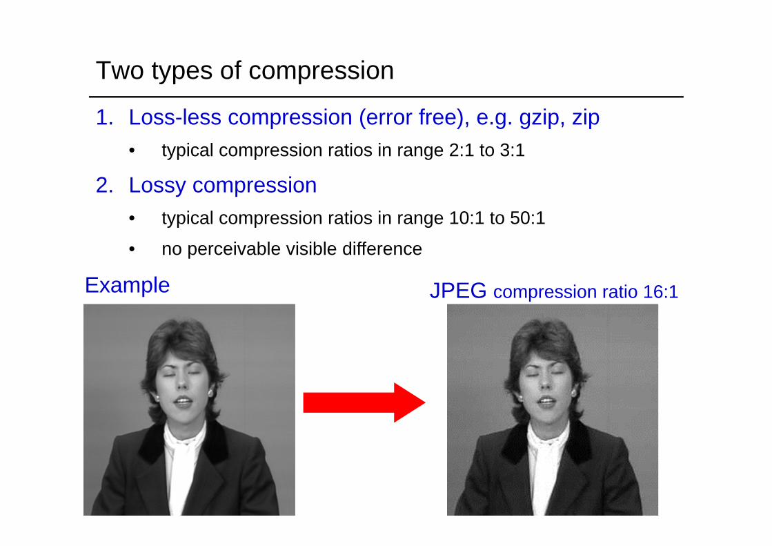
Two types of compression

1. Loss-less compression (error free), e.g. gzip, zip• typical compression ratios in range 2:1 to 3:1

2. Lossy compression• typical compression ratios in range 10:1 to 50:1

• no perceivable visible difference

Example JPEG compression ratio 16:1

Loss-less Compression

Method 1: Run length encoding

Example – white bar length 40

256 x 256 Image = 65536 bytes

Run length encode as

{ (32748,0), (40,255),(32748,0)} = 15 bytes

Compression ratio = 4369

(integer requires 4 bytes, intensity 1 byte)

Extensions: code ramps; code regions

frequency

intensity

Intensity histogram

use short code

use long code

• instead of using same length code (1 byte) for every intensity, use variable length coding

• e.g. 2 bits for most common intensity, longer codes for less common intensities

• Use Huffman coding

Method 2: Coding redundancy

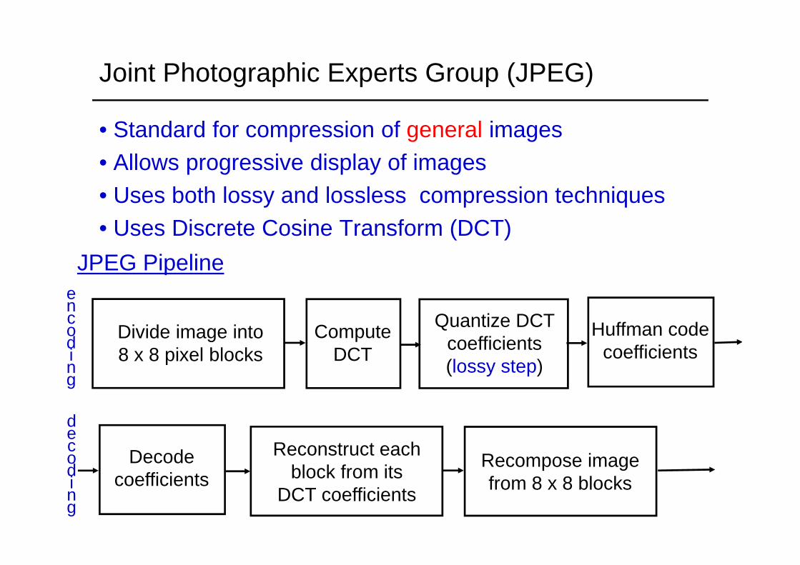
Joint Photographic Experts Group (JPEG)

• Standard for compression of general images• Allows progressive display of images• Uses both lossy and lossless compression techniques• Uses Discrete Cosine Transform (DCT)

Divide image into 8 x 8 pixel blocks

Compute DCT

Quantize DCT coefficients (lossy step)

encoding

Reconstruct each block from its

DCT coefficients

Recompose image from 8 x 8 blocks

decoding

JPEG Pipeline

Huffman code coefficients

Decode coefficients

Discrete Cosine Transform (DCT) (cf Fourier series)

The forward cosine transform is defined as

21 cos

21 cos

,01

01 4, 2

yvN

xuN

yxfyN

xN

NvcucvuF

where

1,...,2,11

,02

1

Nw

wwC for

for

The inverse DCT is defined as

21

21,

01

01

,

yvN

xuN

vuFvCuCvN

uN

yx

coscos

f

8 x 8 basis images for each block

divided into 8 x 8 blocks

JPEG Quantization Step

Example normalization matrix

Z(u,v)out(u,v) = round(F(u,v)/Z(u,v))

• Z(u,v) chosen to weight coefficients which are visually salient

• scale Z(u,v) to alter compression quality

DCT coefficients normalization normalized & denormalized & F(u,v) quantized quantized

out(u,v)

JPEG performance

original CR: 12:1 16:1 21:1Bytes: 65536 5675 4016 3158

CR: 25:1 33:1 41:1 48:1Bytes: 2643 2007 1613 1373

Note “blocking artifacts”

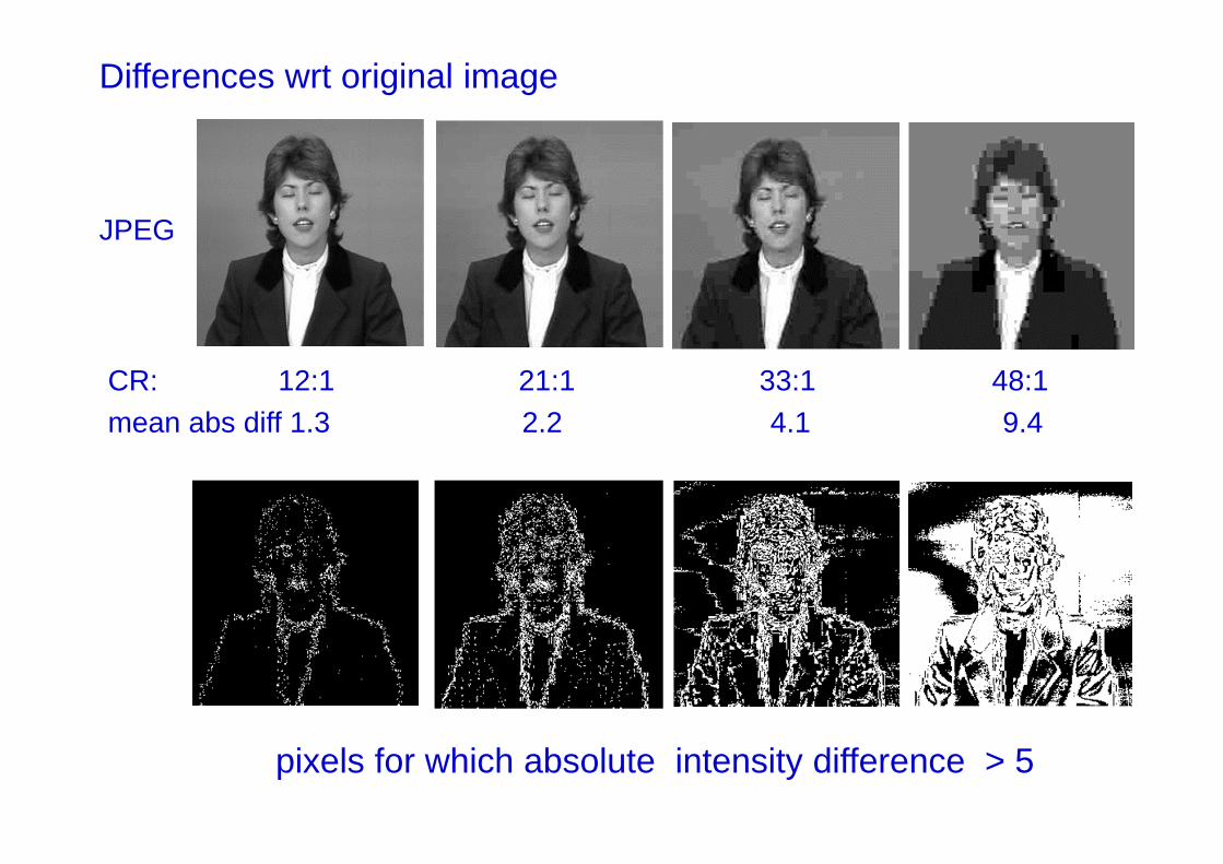
CR: 12:1 21:1 33:1 48:1mean abs diff 1.3 2.2 4.1 9.4

pixels for which absolute intensity difference > 5

Differences wrt original image

JPEG

Non-linear filters

Non-linear filters

• Non-linear filters are more powerful than linear filters, e.g.

• Suppression of non-Gaussian noise, e.g. spikes

• Edge preserving properties

• Examples include median filters, and morphological filters

Median filter

Definition1. rank-order neighbourhood intensities2. select middle value

In 1DThe median of 2N+1 samples is the value which has N smaller

or equal values, and N larger or equal to it.Example

{ 5, 7, 3, 4, 5, 19, 6, 4, 9 } { 3, 4, 4, 5, 5, 6, 7, 9, 19 }Median of set = 5

Note, “odd man out” effect: { 1, 1, 1, 7, 1, 1, 1 }

sort

{ ?, 1, 1, 1, 1, 1, ? }

median width 3

filters have width 5

Median filter • no new grey values are created• edge is preserved• spike is removed

• A median filter operates over a window by selecting the median intensity in the window

Median filter in 2D

Source: K. Grauman

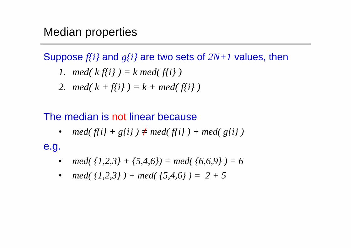
Median properties

Suppose f{i} and g{i} are two sets of 2N+1 values, then1. med( k f{i} ) = k med( f{i} )2. med( k + f{i} ) = k + med( f{i} )

The median is not linear because• med( f{i} + g{i} ) = med( f{i} ) + med( g{i} )

e.g.• med( {1,2,3} + {5,4,6}) = med( {6,6,9} ) = 6• med( {1,2,3} ) + med( {5,4,6} ) = 2 + 5

2D median filter, 3 x 3 neighbourhood

• sharpens edges, reduces noise, but …• generates jagged edges

Gaussian noise

MedianGaussian

Gaussian: upper lip smoother, eye better preserved

Comparison with Gaussian filter

Gaussian noise

10 times 3 X 3 median

• patchy effect• important details lost (e.g. ear-ring)

Salt and Pepper noise

Gaussian = 1 pixel

3 x 3 median

Median filter

Salt and pepper noise

Median filtered

Source: M. Hebert

Plots of a row of the image

Matlab: output im = medfilt2(im, [h w]);

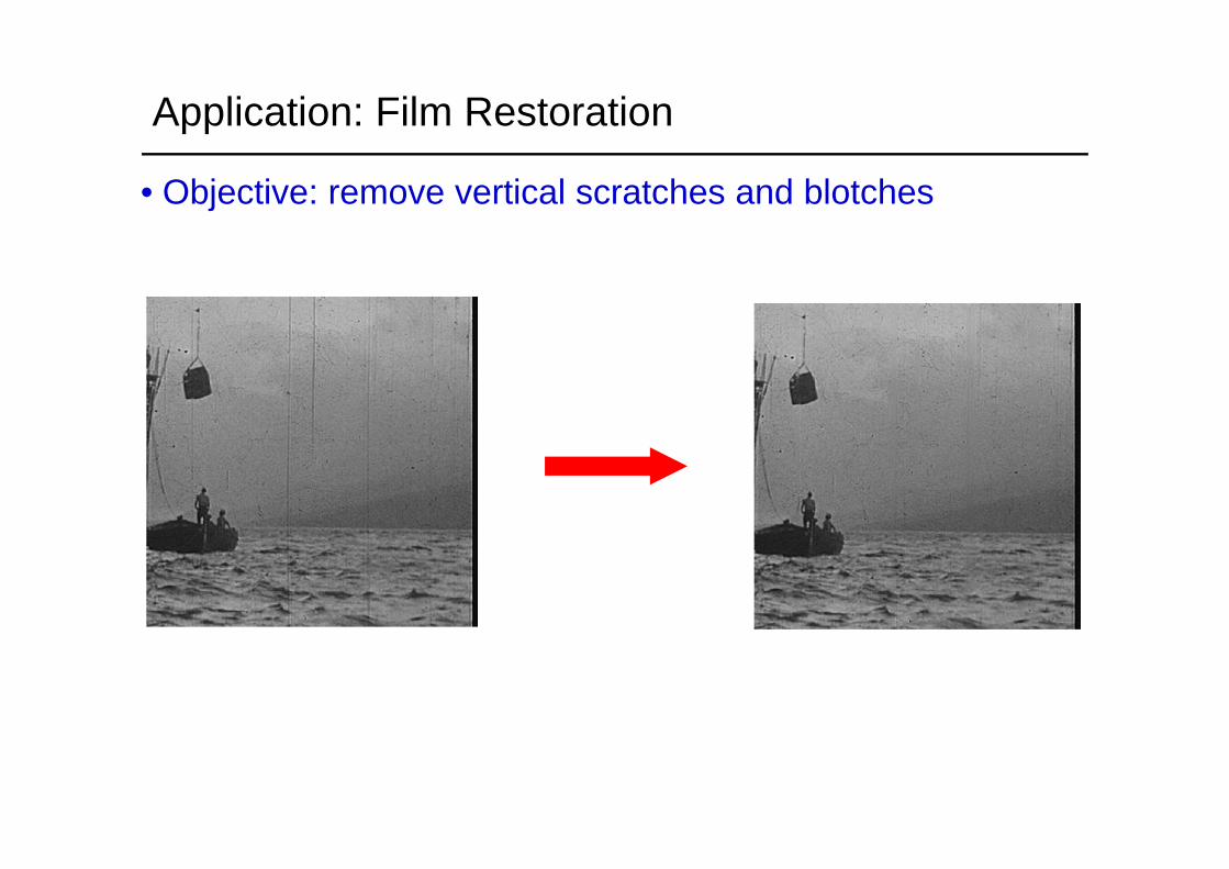
Application: Film Restoration

• Objective: remove vertical scratches and blotches

Bilateral filtering

Gaussian filter = 2

Gaussian filter = 4

Spatial averaging removes noise and blurs edges

6

6

f(x) + n(x)

Can we remove noise but not blur edges?

pq

filtering f(x,y) with a Gaussian filter h(x,y)

for a pixel at p, rewrite this as a weighted average

In(p) =Xq∈S

Gσ(||p− q||)I(q)

over the support of the filter S, where

Gσ(x) = e− x2

2σ2

Inormalization

factor

new

Bilateral filter

Same idea: weighted average of neighbouring pixels but withan additional weighting term

In(p) =1

W

Xq∈S

Gσs(||p−q||)Gσr(|I(p)−I(q)|)I(q)

spatial weight

range weight

1D illustration

pixelintensity

pixel position

In(p) =1

W

Xq∈S


1D illustration

pixelintensity

pixel position

p

Only pixels close in space and in range are considered

In(p) =1

W

Xq∈S


range

spatial

Gaussian blur vs bilateral Filter

Gaussian blur

Bilateral filter

range

p

p

q

q

spatial

spatial

qqpp

output input

pp

reproduced from [Durand 02]

In(p) =1

W

Xq∈S


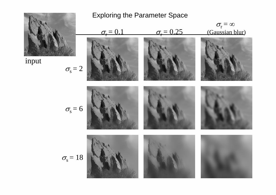
s = 2

s = 6

s = 18

r = 0.1 r = 0.25r =

(Gaussian blur)

input

Exploring the Parameter Space

Basic denoising

Noisy input Bilateral filter 7x7 window

Non-Local Means Denoising


Key idea: to denoise a pixel p use patches in the image with similar neighbourhoods

A. Buades, B. Coll, J.M. Morel "A non local algorithm for image denoising”, CVPR 2005

Image self-similarity

Algorithm:• Select similar (low distance) neighbourhoods to p’s, where the distance

between two neighbourhoods is the Gaussian weighted squared sum of differences

• Compute a Gaussian weighted sum of the centralpixel values as


Assume that if the neighbourhoods are similar, then the central pixel value is also similar (apart from noise)

where Φ is the set of neighbourhoods andW =Pq∈Φ e

−d(Np,Nq)h2

pNp

Nq

d(Np, Nq)

In(p) =1

W

Xq∈Φ

e−d(Np,Nq)

h2 I(q) q

d(Np, Nq) e−d(Np,Nq)

h2

black = low

Parameters:• neighbourhood size: 5 x 5• search region: 7 x 7

Removing film grainoriginal

Removing film graindenoised

Inpainting

Inpainting techniques

• Automated texture generation to fill in regions

Texture Synthesis

Texture sample

Output

Efros & Leung, ICCV 1999

Synthesizing One Pixel

• Select patches with similar neighbourhoods• Choose a central pixel value randomly from this set

pinput image

synthesized image

Slide from Alyosha Efros, ICCV 1999

Neighborhood Window

input


Hole Filling


A Cautionary Note …

Removal of Nikolai Yezhov

Removal of foreground objects using inpainting

original frame


inpainted frame


original frame


inpainted frame

There is much more …

• Image reorganization, e.g. using the patch transform

scale

retarget

• Image retargettinge.g. change of aspect ratio withoutlosing or distorting semantic content

Lecture 4: Non-linear filters & Image Compression

Documents