Lecture 4: Morphological Image Processing Harvey Rhody Chester F. Carlson Center for Imaging Science Rochester Institute of Technology [email protected] September 15, 2005 Abstract We will develop morphological image processing techniques that use combinations and sequences of operations. These techniques are useful in a wide range of applications. DIP Lecture 4

Welcome message from author
This document is posted to help you gain knowledge. Please leave a comment to let me know what you think about it! Share it to your friends and learn new things together.
Transcript

Lecture 4: Morphological Image Processing
Harvey RhodyChester F. Carlson Center for Imaging Science
Rochester Institute of [email protected]
September 15, 2005
AbstractWe will develop morphological image processing techniques that
use combinations and sequences of operations. These techniques areuseful in a wide range of applications.
DIP Lecture 4

Morphological Algorithms
• Boundary Extraction
• Region Filling
• Connected Components
• Hit-or-Miss Transform
• Convex Hull
• Thinning and Thickening
Boundary extraction was done in Lecture 3.
DIP Lecture 4 1

Region Filling
Develop an algorithm to fill in bounded regions of background color.
1. Let B be a structuring element of type N4, Nd or N8, depending on thedesired connectivity.
2. Select a pixel p inside a background color region.
3. Initialize X0 to be an array of background pixels except X0[p] = 1.
4. Perform the iteration
Xk = (Xk−1 ⊕B)⋂
Ac for k = 1, 2, 3, . . .
until Xk = Xk−1.
DIP Lecture 4 2

Region Filling Program
Function Region Fill,A,start,filter=B,max iterations=max iterations
IF n params() LT 2 THEN Message,’Too Few Arguments to Function’IF NOT KEYWORD SET(B) THEN B=[[0b,1b,0b],[1b,1b,1b],[0b,1b,0b]]IF NOT KEYWORD SET(max iterations) THEN max iterations=10000L
sa=Size(A,/dim)X=BytArr(sa[0],sa[1]) & X[start]=1bY=BytArr(sa[0],sa[1])Ac=A EQ 0count=0WHILE ((min(X EQ Y) EQ 0) AND (count LT max iterations)) DO BEGIN
count=count+1Y=XX=Dilate(Y,B) AND Ac
ENDWHILERETURN,XEND
DIP Lecture 4 3

Example: Connected Regions in Maze
DIP Lecture 4 4

Example: Connected Regions in Maze
DIP Lecture 4 5

Connected Components
We have used a labeling technique to find connected components. Here we will examine a
morphological technique based on set operations.
1. Let A be a binary image and let Y be a connected component in A. Assume that a
point p ∈ Y is known.
2. Let B be the structuring element
B =
24
1 1 1
1 1 1
1 1 1
35
3. Let X0 = p and perform the iteration
Xk =�Xk−1 ⊕ B
�∩ A for k = 1, 2, 3, . . .
until Xk = Xk−1
DIP Lecture 4 6

Example: G&W Figure 9.17
Search for the connected component in the figure
to the right starting at the red pixel.
The iteration results are shown in the sequence of
images below.
DIP Lecture 4 7

Connected Components Program
Function morph cc,A,start,filter=filter,max iterations=max iterations,count=count
IF n params() LT 2 THEN Message,’Too Few Arguments to Function’
IF KEYWORD SET(filter) THEN B=filter ELSE B=[[1b,1b,1b],[1b,1b,1b],[1b,1b,1b]]
IF NOT KEYWORD SET(max iterations) THEN max iterations=10000L
sa=Size(A,/dim)
X=BytArr(sa[0],sa[1]) & X[start]=1b
Y=BytArr(sa[0],sa[1])
count=0
WHILE ((min(X EQ Y) EQ 0) AND (count LT max iterations)) DO BEGIN
count=count+1
Y=X
X=Dilate(Y,B) AND A
ENDWHILE
RETURN,X
END
DIP Lecture 4 8

Connected Components Search
Let A be a N ×M binary image.
1. Initialization
(a) Set B = A
(b) Set C = 0 (an N ×M array of zeros.)
(c) ib=Where(B NE 0)
(d) k=1
2. Iteration: While Min(ib) GE 0
(a) X=morph cc(B,ib[0])
(b) C=C+kX & k=k+1
(c) B=B AND (X EQ 0)
(d) ib=Where(B NE 0) (returns ib=-1 when B is empty)
DIP Lecture 4 9

Finding All Connected Components
Shown below is an original image, a color-coded image showing the connected components,
and an index color palette.
DIP Lecture 4 10

Hit-or-Miss Transform
The morphological hit-or-miss transform is a basic tool for shape detection.
The transform is produced by eroding an image with one structuring element and its
complement with another structuring element and then combining the results.
If A is an image and B = (B1, B2) is a pair of structuring elements, then the H-M
transform is
(A ~ B) = (A B1) ∩ (Ac B2)
DIP Lecture 4 11
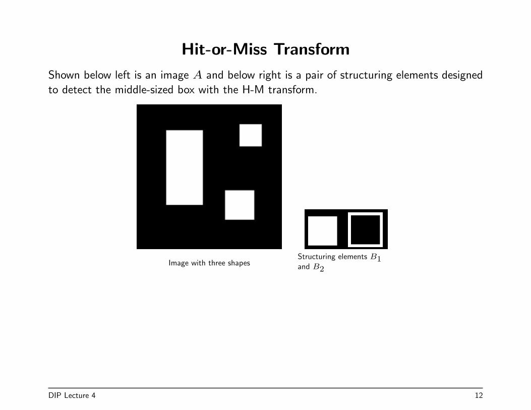
Hit-or-Miss Transform
Shown below left is an image A and below right is a pair of structuring elements designed
to detect the middle-sized box with the H-M transform.
Image with three shapesStructuring elements B1and B2
DIP Lecture 4 12

Hit-or-Miss Transform
Original Image A (A B1) B1 and B2
(Ac B2) (A ~ B) = (A B1) ∩ (Ac B2)
DIP Lecture 4 13

Example 1
Use the H-M transform to find the small squares in the image below. Assume that B1 and
B2 are of the exact size to fit the small squares.
Original ImageStructuring elements B1 and B2.(Not to scale)
DIP Lecture 4 14

Example 1 (cont)
Original Image A C1 = (A B1) Ac
C2 = (Ac B2) (A ~ B) = C1 ∩ C2 Detected objects shown in red.
DIP Lecture 4 15

Example 2
Find the three different kinds of objects in the image on the left.
To find the small boxes use B = (S1, S2), to find the hollow boxes use C = (S2, S3)
and to find the large boxes use D = (S4, S5).
S1
S2
S3
S4
S5
Original image Search results
DIP Lecture 4 16

Convex Hull
A set A is said to be convex if any two elements can be joined by a straight path that
does not go outside the set.
The convex hull H of a set S is the smallest convex set such that S ⊆ H.
The set difference H − S = H ∩ Sc is the convex deficiency of S.
The convex set and convex deficiency are needed in many applications.
DIP Lecture 4 17

Convex Hull Algorithm
The convex hull algorithm uses the H-M transform with four sets of structuring elements,
(Bi, C) as given by the arrays below.
100 111 001 000 000100 000 001 000 010100 000 001 111 000B1 B2 B3 B4 C
1. Initialize four arrays Xi0 = A, i =
1, 2, 3, 4.
2. Compute Xik = (Xi
k−1 ~ Bi) ∪ A
until Xik = Xi
k−1. Let Xiconv be the
“converged” value.
3. C(A) =S4
i=1 Xiconv
4. Trim C(A) to the bounding box of the
component.
DIP Lecture 4 18

Example: G&W Figure 9.19
The set shown below corresponds to G&W Figure 9.19. The goal is to find the convex hull
H for this set.
DIP Lecture 4 19

Example (cont)
Shown below is the sequence of arrays X1k. It converges in four steps.
DIP Lecture 4 20

Example (cont)
Shown below is the sequence of arrays X2k. It converges in two steps.
DIP Lecture 4 21
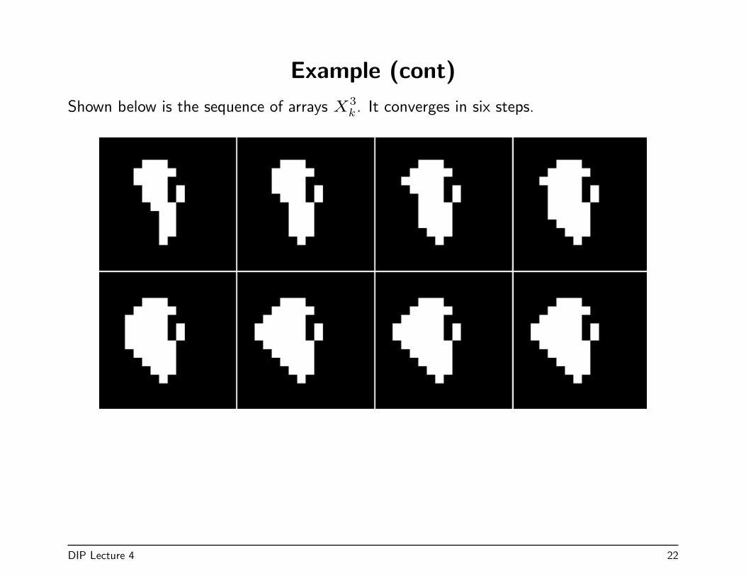
Example (cont)
Shown below is the sequence of arrays X3k. It converges in six steps.
DIP Lecture 4 22

Example (cont)
Shown below is the sequence of arrays X4k. It converges in two steps.
DIP Lecture 4 23

Example (cont)
The union of the four converged arrays is shown below left. The original set is in white
and the convex set is in red. The convex set may be trimmed to the bounding box of the
original set to form the convex hull H as shown on the right in green and white.
DIP Lecture 4 24

Morphological Thinning
Thinning removes pixels from a set until only a narrow set remains. It is used to reveal set
structure in recognition applications.
Thinning uses a sequence of structuring elements
B = {B1, B
2, . . . , B
n}
Basic thinning operation
1. Let Xn = A and Y = X0 = [0]N×M
2. Repeat while Xn 6= Y
Y = Xn
X0 = Xn
Xi = Xi−1 ∩ (Xi−1 ~ Bi)c
for i = 1, 2, . . . , n
DIP Lecture 4 25
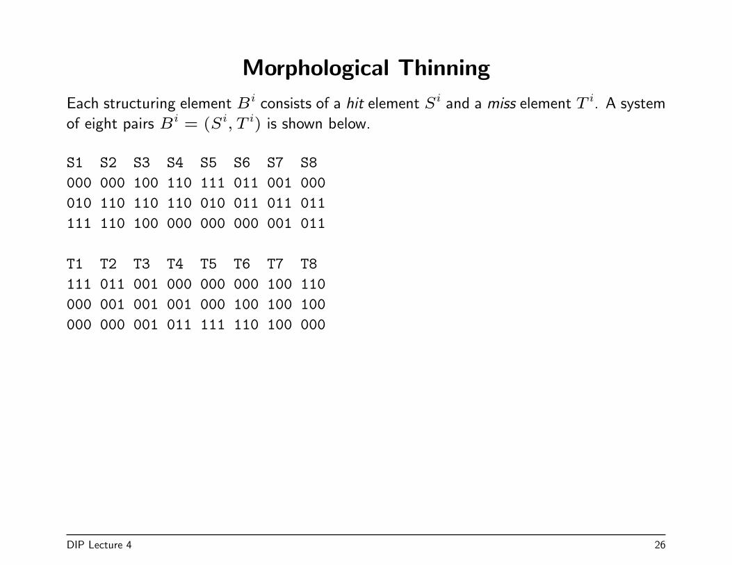
Morphological Thinning
Each structuring element Bi consists of a hit element Si and a miss element T i. A system
of eight pairs Bi = (Si, T i) is shown below.
S1 S2 S3 S4 S5 S6 S7 S8000 000 100 110 111 011 001 000010 110 110 110 010 011 011 011111 110 100 000 000 000 001 011
T1 T2 T3 T4 T5 T6 T7 T8111 011 001 000 000 000 100 110000 001 001 001 000 100 100 100000 000 001 011 111 110 100 000
DIP Lecture 4 26

Example: G&W Figure 9.21
The original image is shown in the upper left. One pass of the algorithm is then made,
with each structuring element used one time. For each Bi, the Si is shown in white and
the T i is shown in red.
A X1 X2
X3 X4 X5
X6 X7 X8
B1 B2
B3 B4 B5
B6 B7 B8
DIP Lecture 4 27
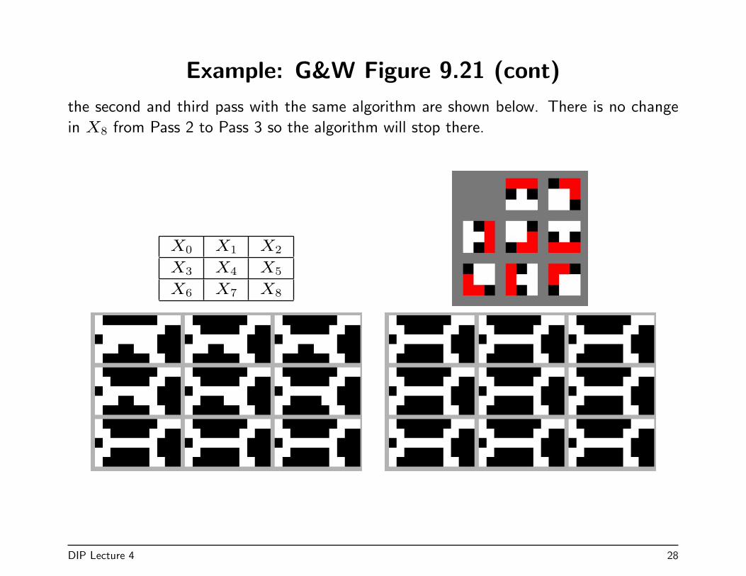
Example: G&W Figure 9.21 (cont)
the second and third pass with the same algorithm are shown below. There is no change
in X8 from Pass 2 to Pass 3 so the algorithm will stop there.
X0 X1 X2
X3 X4 X5
X6 X7 X8
DIP Lecture 4 28
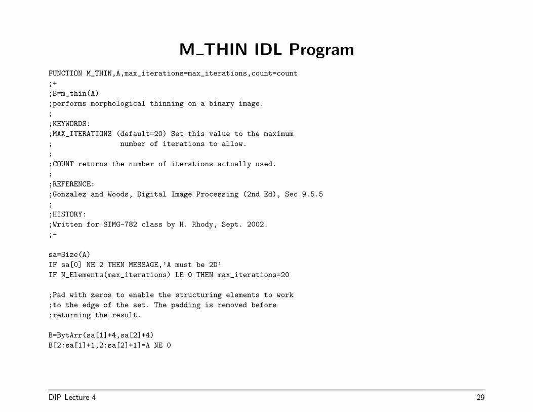
M THIN IDL ProgramFUNCTION M_THIN,A,max_iterations=max_iterations,count=count;+;B=m_thin(A);performs morphological thinning on a binary image.;;KEYWORDS:;MAX_ITERATIONS (default=20) Set this value to the maximum; number of iterations to allow.;;COUNT returns the number of iterations actually used.;;REFERENCE:;Gonzalez and Woods, Digital Image Processing (2nd Ed), Sec 9.5.5;;HISTORY:;Written for SIMG-782 class by H. Rhody, Sept. 2002.;-
sa=Size(A)IF sa[0] NE 2 THEN MESSAGE,’A must be 2D’IF N_Elements(max_iterations) LE 0 THEN max_iterations=20
;Pad with zeros to enable the structuring elements to work;to the edge of the set. The padding is removed before;returning the result.
B=BytArr(sa[1]+4,sa[2]+4)B[2:sa[1]+1,2:sa[2]+1]=A NE 0
DIP Lecture 4 29

M THIN (cont);STRUCTURING ELEMENTSS1=[[0b,0b,0b],[0b,1b,0b],[1b,1b,1b]]T1=[[1b,1b,1b],[0b,0b,0b],[0b,0b,0b]]
S2=[[0b,0b,0b],[1b,1b,0b],[1b,1b,0b]]T2=[[0b,1b,1b],[0b,0b,1b],[0b,0b,0b]]
S3=Reverse(Transpose(S1),1)T3=Reverse(Transpose(T1),1)
S4=Reverse(Transpose(S2),1)T4=Reverse(Transpose(T2),1)
S5=Reverse(S1,2)T5=Reverse(T1,2)
S6=Reverse(S4,1)T6=Reverse(T4,1)
S7=Reverse(S3,1)T7=Reverse(T3,1)
S8=Reverse(S2,1)T8=Reverse(T2,1)
DIP Lecture 4 30

M THIN (cont)X=BY=BYTARR(sa[1]+4,sa[2]+4)count=0WHILE MAX(X NE Y) GT 0 AND count LT max_iterations DO BEGINY=XX=Y AND NOT Morph_HitOrMiss(X,S1,T1)X=X AND NOT morph_HitOrMiss(X,S2,T2)X=X AND NOT morph_HitOrMiss(X,S3,T3)X=X AND NOT morph_HitOrMiss(X,S4,T4)X=X AND NOT morph_HitOrMiss(X,S5,T5)X=X AND NOT morph_HitOrMiss(X,S6,T6)X=X AND NOT morph_HitOrMiss(X,S7,T7)X=X AND NOT morph_HitOrMiss(X,S8,T8)count=count+1ENDWHILE
RETURN,X[2:sa[1]+1,2:sa[2]+1]END
DIP Lecture 4 31

Example: Thin the Blobs
The basic structure is captured by the thinned objects (red). The small ends could be removed by further processing to refine theresult.
DIP Lecture 4 32

Morphological Thickening TransformThickening is the morphological dual of thinning and is defined by
A� B = A ∪ (A ~ B)
The algorithm can be programmed directly from the definition. However, it has been found to be more effective to do thickeningby thinning Ac.
1. Let C = Ac
2. Let D be thinned (using m thin, for example)
3. T = Dc is the thickened object.
DIP Lecture 4 33

Example: G&W Figure 9.22The steps in the thickening algorithm are illustrated in the figure below.
A C = Ac
D T = Dc
DIP Lecture 4 34
Related Documents