Lecture 3: Stochastic Differential Equations › ~song › Gene Golub Summer... · Linear stochastic differential equations The geometric Brownian motion X t = ˘e ˙ 2 2 t+˙Bt solves

Lecture 3: Stochastic Differential Equations

David Nualart

Department of MathematicsKansas University

Gene Golub SIAM Summer School 2016Drexel University

David Nualart (Kansas University) July 2016 1 / 54

Strong solutions

Let B = Bjt , t ≥ 0, j = 1, . . . ,d be a d-dimensional Brownian motion

and ξ an m-dimensional random vector independent of B.

Let Ft be the σ-field generated by Bs,0 ≤ s ≤ t , ξ and the null sets.

Consider measurable coefficients bi (t , x) and σij (t , x), 1 ≤ i ≤ m,1 ≤ j ≤ d from [0,∞)× Rm to R.

Our aim to give a meaning to the stochastic differential equation on Rm :

dX it = bi (t ,Xt )dt +

d∑j=1

σij (t ,Xt )dBjt , 1 ≤ i ≤ m (1)

with initial condition X0 = ξ.


DefinitionWe say that an adapted and continuous process X = Xt , t ≥ 0 is a solutionto equation (1) if for all t ≥ 0,

Xt = ξ +

∫ t

0b(s,Xs)ds +

∫ t

0σ(s,Xs)dBs, a.s.

or

X it = ξi +

∫ t

0bi (s,Xs)ds +

d∑j=1

∫ t

0σij (s,Xs)dBj

s, 1 ≤ i ≤ m, a.s.

b is called the drift and σ is called the diffusion coefficient.


TheoremSuppose that the coefficients are locally Lipschitz in the space variable, thatis, for each N ≥ 1, there exists KN > 0 such that for each ‖x‖, ‖y‖ ≤ N andt ≥ 0

‖b(t , x)− b(t , y)‖+ ‖σ(t , x)− σ(t , y)‖ ≤ KN‖x − y‖.

Then, two solutions with the same initial condition coincide almost surely(strong uniqueness holds).

In the absence of the locally Lipschitz condition equation (1) might fail tobe solvable or have multiple solutions.

Example : Xt =∫ t

0 |Xs|αds, where α ∈ (0,1). Then Xt = 0 is a solutionand also, for any s ≥ 0,

Xt =

(t − sβ

)β1[s,∞)(t), β = 1/(1− α),

is also a solution.


Lemma (Gronwall lemma)Let u be a nonnegative continuous function on [0,∞) such that

u(t) ≤ α(t) +

∫ t

0β(s)u(s)ds, t ≥ 0

with β ≥ 0 and α non-decreasing. Then,

u(t) ≤ α(t) exp

(∫ t

0β(s)ds

), t ≥ 0.

In particular, if α and β are constant, we get

u(t) ≤ αeβt .


Proof :

Let X and X two solutions. Define

Sn = inft ≥ 0 : ‖Xt‖ ≥ n or ‖Xt‖ ≥ n.

Clearly Sn are stopping times such that Sn ↑ ∞.

Then,

E‖Xt∧Sn − Xt∧Sn‖2 ≤ 2E

[∫ t∧Sn

0‖b(u,Xu)− b(u, Xu‖du

]2

+2Em∑

i=1

∣∣∣∣∣∣d∑

j=1

∫ t∧Sn

0(σij (u,Xu)− σij (u, Xu))dBj

u

∣∣∣∣∣∣2

≤ 2tE∫ t∧Sn

0‖b(u,Xu)− b(u, Xu‖2du

+2E∫ t∧Sn

0‖σ(u,Xu)− σ(u, Xu‖2du.


Using the local Lipschitz property, we obtain for any t ≥ 0,

E‖Xt∧Sn − Xt∧Sn‖2 ≤ 2(t + 1)K 2

n

∫ t

0E‖Xu∧Sn − Xu∧Sn‖

2du.

Then g(t) = E‖Xt∧Sn − Xt∧Sn‖2 satisfies

g(t) ≤ 2(t + 1)K 2n

∫ t

0g(u)du,

which, by Gronwall’s lemma, implies that g = 0.

Letting n→∞ we conclude that Xt = Xt .


A local Lipschitz condition is not sufficient to guarantee global existenceof a solution.Example :

Xt = 1 +

∫ t

0X 2

s ds.

the solution is Xt = 11−t , which explodes as t ↑ 1.


Exercise : Given x ∈ Rm, we can find a strictly positive stopping time τand a stochastic process Xt , t < τ such that

Xt = x +

∫ t

0b(s,Xs)ds +

∫ t

0σ(s,Xs)dBs, t < τ.

The process Xt , t < τ is unique in the sense that if ρ is another strictlypositive stopping time and Yt , t < ρ satisfies

Yt = x +

∫ t

0b(s,Ys)ds +

∫ t

0σ(s,Ys)dBs, t < ρ,

then ρ ≤ τ and for every t ≥ 0, Yt1t<ρ = Xt1t<ρ.


TheoremSuppose that the coefficients b and σ satisfy the global Lipschitz and lineargrowth conditions :

‖b(t , x)− b(t , y)‖+ ‖σ(t , x)− σ(t , y)‖ ≤ K (‖x − y‖,‖b(t , x)‖2 + ‖σ(t , x)‖2 ≤ K 2(1 + ‖x‖2),

for every x , y ∈ Rm, t ≥ 0. Suppose also that

E‖ξ‖2 <∞.

Then, there exist a unique solution such that for any T > 0

E

(sup

0≤t≤T‖Xt‖2

)≤ CT ,K (1 + E‖ξ‖2),

where CT ,K depends on T and K .


Proof :

(i) Define the Picard iterations by putting X (0)t = ξ and for k ≥ 0,

X (k+1)t = ξ +

∫ t

0b(s,X (k)

s )ds +

∫ t

0σ(s,X (k)

s )dBs.

It is easy to check that

E

(sup

0≤t≤T‖X (1)

t ‖2

)≤ CT ,K (1 + E‖ξ‖2).

Then X (k+1)t − X (k)

t = Vt + Mt , where

Vt =

∫ t

0[b(s,X (k)

s )− b(s,X (k−1)s )]ds

and

Mt =

∫ t

0[σ(s,X (k)

s )− σ(s,X (k−1)s )]dBs.


(ii) By the maximal inequality for square integrable martingales,

E

[sup

0≤t≤T‖Mt‖2

]≤ 4E

∫ T

0‖σ(s,X (k)

s )− σ(s,X (k−1)s )‖2ds

≤ 4K 2∫ T

0E‖X (k)

s − X (k−1)s ‖2ds.

On the other hand,

E

[sup

0≤t≤T‖Vt‖2

]≤ K 2T

∫ T

0E‖X (k)

s − X (k−1)s ‖2ds,

which leads to

E

[sup

0≤t≤T‖X (k+1)

t − X (k)t ‖

2

]≤ L

∫ T

0E‖X (k)

s − X (k−1)s ‖2ds,

where L = 2K 2(4 + T ).


(iii) By iteration,

E

[sup

0≤t≤T‖X (k+1)

t − X (k)t ‖

2

]≤ C∗

(LT )k

k !,

where C∗ = E[max0≤t≤T ‖X (1) − ξ‖2

]<∞. Consider the Banach space

ET of continuous adapted processes X = Xt , t ∈ [0,T ] such that

‖X‖ET :=

(E

(sup

0≤t≤T‖Xt‖2

)) 12

<∞.

Then the sequence X (k) converges in ET to a limit X which satisfies theequation.


Under the assumptions of the theorem, if E‖ξ‖p <∞ for some p ≥ 2,then the solution satisfies the following moments estimate,

E

[sup

t∈[0,T ]

‖Xt‖p

]≤ CT ,K ,p(1 + E [‖ξ‖p]),

where C depends on K , T and p.The proof uses Burkholder-David-Gundy inequality.


Linear stochastic differential equations

The geometric Brownian motion

Xt = ξe(µ−σ2

2

)t+σBt

solves the linear SDE

dXt = µXtdt + σXtdBt .

More generally, the solution of the homogeneous linear SDE

dXt = b(t)Xtdt + σ(t)XtdBt ,

where b(t) and σ(t) are continuous functions, is

Xt = ξ exp[∫ t

0

(b(s)− 1

2σ2(s)

)ds +

∫ t0 σ(s)dBs

].


Ornstein-Uhlenbeck process

Consider the SDE (Langevin equation)

dXt = a (µ− Xt ) dt + σdBt

with initial condition X0 = x , where a, σ > 0 and µ is a real number.

The process Yt = Xteat , satisfies

dYt = aXteatdt + eatdXt = aµeatdt + σeatdBt .

Thus,

Yt = x + µ(eat − 1) + σ

∫ t

0easdBs,

which implies

Xt = µ+ (x − µ)e−at + σe−at∫ t

0 easdBs.


The process Xt is Gaussian with mean and covariance given by :

E(Xt ) = µ+ (x − µ)e−at ,

Cov (Xt ,Xs) = σ2e−a(t+s)E

[(∫ t

0ear dBr

)(∫ s

0ear dBr

)]

= σ2e−a(t+s)∫ t∧s

0e2ar dr

=σ2

2a

(e−a|t−s| − e−a(t+s)

).

The law of Xt is the normal distribution

N(µ+ (x − µ)e−at ,

σ2

2a(1− e−2at))

and it converges, as t tends to infinity to the normal law

ν = N(µ,σ2

2a).

This distribution is called invariant or stationary.

Exercise : Show that if L(ξ) = ν, then Xt has law ν, ∀t ≥ 0.David Nualart (Kansas University) July 2016 17 / 54

General linear SDEs

Consider the equation

dXt = (a(t) + b(t)Xt ) dt + (c(t) + d(t)Xt ) dBt ,

with initial condition ξ = x , where a, b, c and d are continuous functions.The solution to this equation is given by

Xt = Ut

(x +

∫ t

0[a(s)− c(s)d(s)] U−1

s ds +

∫ t

0c(s) U−1

s dBs

),

where

Ut = exp

(∫ t

0b(s)ds +

∫ t

0d(s)dBs −

12

∫ t

0d2(s)ds

).

Proof : Write Xt = UtVt , where dVt = α(t)dt + β(t)dBt , and find α and β.


Stochastic flows

Suppose that the coefficients are globally Lipschitz with lineargrowth.Denote by X x

t the solution with initial condition x ∈ Rm.

PropositionLet T > 0. For every p ≥ 2, there exists a constant Cp,T such that for each0 ≤ s ≤ t ≤ T and x , y ∈ Rm,

E(‖X x

t − X ys ‖p) ≤ Cp,T (‖x − y‖p + |t − s|p/2).

As a consequence, there exists a version X xt , t ≥ 0, x ∈ Rm of the process

X xt , t ≥ 0, x ∈ Rm which is continuous in (t , x) ∈ [0,∞)× Rm.

The continuous process of continuous maps Ψt : x → X xt is called the

stochastic flow associated to equation (1).


Denote by X t,xs , s ≥ t the solution to equation (1) starting at time t with

initial condition x :

X t,xs = x +

∫ s

tb(θ,X t,x

θ )dθ +

∫ s

tσ(θ,X t,x

θ )dBθ, s ≥ t .

One can also snow that there is a version of the processX t,x

s , s ≥ t ≥ 0, x ∈ Rm which is continuous in all its variables.

Proposition (Flow property)If s ≥ t ,

X 0,xs = X t,X 0,x

ts , a.s.


Proof :

Almost surely, for any y ∈ Rm,

X t,ys = y +

∫ s

tb(θ,X t,y

θ )dθ +

∫ s

tσ(θ,X t,y

θ )dBθ.

Substituting y by X 0,xt yields

X t,X 0,xt

s = X 0,xt +

∫ s

tb(θ,X t,X 0,x

tθ )dθ +

∫ s

tσ(θ,X t,X 0,x

tθ )dBθ.

On the other hand, X 0,xs is also a solution to this equation for s ≥ t

because

X 0,xs = X 0,x

t +

∫ s

tb(θ,X 0,x

θ )dθ +

∫ s

tσ(θ,X 0,x

θ )dBθ.

Then, the uniqueness of the solution implies the result.


Markov property

TheoremThe solution Xt is a Markov process with respect to the Brownian filtration Ft .Furthermore, for any f ∈ Cb(Rm) and t ≥ s, we have

E [f (Xt )|Fs] = (Ps,t f )(Xs),

where Ps,t f (x) = E [f (X s,xt )].

If the coefficients are time independent, Ps,t can be written as Pt−s,where Pt , t ≥ 0 is the semigroup of operators with infinitesimalgenerator

L =12

m∑i,k=1

aik∂2f

∂xi∂xk+

m∑i=1

bi∂f∂xi

,

where aik =∑d

j=1 σijσkj .


Sketch of the proof :

(i) X s,xt is a measurable function of x and the Brownian incrementsBs+u − Bs,u ≥ 0, that is

X s,xt = Φ(x ,Bs+u − Bs,u ≥ 0).

(ii) This implies, by the flow property, that

X 0,xt = Φ(X 0,x

s ,Bs+u − Bs,u ≥ 0),

where X 0,xs is Fs-measurable and Bs+u − Bs,u ≥ 0 is independent of

Fs.

(iii) Therefore,

E [f (Φ(X 0,xs ,Bs+u − Bs,u ≥ 0))|Fs] = E [f (Φ(y ,Bs+u − Bs,u ≥ 0))]|y=X 0,x

s,

which yields the result.


Numerical approximations

Euler’s scheme :

Fix T > 0 and set ti = iTn , = 0,1, . . . ,n. The Euler’s method consists in

the recursive scheme :

X (n)(ti ) = X (n)(ti−1) + b(ti−1,X (n)(ti−1))Tn

+ σ(ti−1,X (n)(ti−1))∆Bi ,

i = 1, . . . ,n, where ∆Bi = Bti − Bti−1 .

The initial value is X (n)0 = x0.

Inside the interval (ti−1, ti ) the value of the process X (n)t is given by linear

interpolation, or by the equation

X (n)t = x0 +

∫ t

0b(κn(s),Xκn(s)) +

∫ t

0σ(κn(s),Xκn(s))dBs,

where κn(s) = ti−1 if s ∈ [ti−1, ti ).


Proposition

The error of the Euler’s method is of order n−12 :√

E[(

XT − X (n)T

)2]≤ C

√Tn.

In order to simulate a trajectory of the solution using Euler’s method, itsuffices to simulate the values of n independent random variables

ξ1, . . . , ξn with distribution N(0,1), and replace ∆Bi by√

Tn ξi .


Milstein scheme :

Euler’s method can be improved by adding a correction term. To simplifywe assume m = d = 1 and that the coefficients are time independent.We can write

X (ti ) = X (ti−1) +

∫ ti

ti−1

b(Xs)ds +

∫ ti

ti−1

σ(Xs)dBs. (2)

Euler’s method is based on the approximations∫ ti

ti−1

b(Xs)ds ≈ b(X (ti−1))Tn,∫ ti

ti−1

σ(Xs)dBs ≈ σ(X (ti−1))∆Bi .


Applying Ito’s formula to the processes b(Xs) and σ(Xs), we obtain

X (ti )− X (ti−1)

=

∫ ti

ti−1

[b(X (ti−1)) +

∫ s

ti−1

(bb′ +

12

b′′σ2)

(Xr )dr

+

∫ s

ti−1

(σb′) (Xr )dBr

]ds

+

∫ ti

ti−1

[σ(X (ti−1)) +

∫ s

ti−1

(bσ′ +

12σ′′σ2

)(Xr )dr

+

∫ s

ti−1

(σσ′) (Xr )dBr

]dBs

= b(X (ti−1))Tn

+ σ(X (ti−1))∆Bi +

∫ ti

ti−1

(∫ s

ti−1

(σσ′) (Xr )dBr

)dBs + Ri,n,

where the term Ri,n is of lower order.


This double stochastic integral can also be approximated by

(σσ′) (X (ti−1))

∫ ti

ti−1

(∫ s

ti−1

dBr

)dBs.

The rules of Ito stochastic calculus lead to∫ ti

ti−1

(∫ s

ti−1

dBr

)dBs =

∫ ti

ti−1

(Bs − Bti−1

)dBs

=12

(B2

ti − B2ti−1

)− Bti−1

(Bti − Bti−1

)− T

2n

=12

[(∆Bi )

2 − Tn

].


The Milstein’s method consists in the recursive scheme :

X (n)(ti ) = X (n)(ti−1) + b(X (n)(ti−1))Tn

+ σ(X (n)(ti−1)) ∆Bi

+12

(σσ′) (X (n)(ti−1))

[(∆Bi )

2 − Tn

].

One can show that the error is of order Tn , that is,√

E[(

XT − X (n)T

)2]≤ C

Tn.


Proposition (Yamada-Watanabe ’71)Consider the 1-dimensional SDE

dXt = b(t ,Xt ) + σ(t ,Xt )dBt ,

where the coefficients have linear growth and satisfy

|b(t , x)− b(t , y)| ≤ K |x − y ||σ(t , x)− σ(t , y)| ≤ h(|x − y |),

with h : [0,∞)→ [0,∞) is strictly increasing, h(0) = 0 and∫ ε

0h−2(x)dx =∞, ∀ε > 0.

Then strong uniqueness holds.

Example : σ(x) = |x |α with α ≥ 12 (Girsanov ’62).


Proof in the case b = 0, σ(x) = |x |α, α ∈ ( 12 ,1] :

Let X and X be two solutions with the same initial condition. ThenY = X − X satisfies

Yt =

∫ t

0

[|Xs|α − |Xs|α

]dBs.

Applying Ito’s formula to ψn(x) such that ψ′′(x) = n1[− 1n ,

1n ]

(x), yields

E [ψn(Yt )] =n2

E

[∫ t

01[− 1

n ,1n ]

(Ys)[|Xs|α − |Xs|α

]2ds

].

which implies

E [ψn(Yt )] ≤ n2

E

[∫ t

01[− 1

n ,1n ]

(Ys)|Ys|2αds

]≤ t

2n1−2α → 0.

Therefore, E [|Yt |] = 0.


Weak solutions

DefinitionA weak solution is a triple (X ,B), (Ω,F ,P) and Ft , such that :

(i) Ft is a filtration in a probability space (Ω,F ,P), right-continuous andcontaining all P-null sets.

(ii) Xt is a continuous m-dimensional adapted process and Bt is anFt -Brownian motion on Rd .

(iii) Equation (1) is satisfied.

The filtration Ft may not be the augmentation of the filtration generatedby B and the initial condition.


Example :

Consider the SDE

Xt =

∫ t

0sgn(Xs)dBs

where sgn(x) = 1(0,∞)(x)− 1(−∞,0](t).

One can construct a weak solution by choosing a Brownian motion Xtand

Bs =

∫ t

0sgn(Xs)dXs.

In this case, strong uniqueness does not hold, but there is uniqueness inlaw of all weak solutions.

The filtration generated by Xt is strictly larger than the filtrationgenerated by Bt (which is the filtration generated by |Xt |).


PropositionConsider the SDE

dXt = b(t ,Xt )dt + dBt , t ∈ [0,T ]

where Bt is a d-dimensional Brownian motion and b : [0,T ]× Rd → Rd

satisfies‖b(t , x)‖ ≤ K (1 + ‖x‖).

Then there is a weak solution for any initial distribution µ.


Proof :

To simplify we assume that the initial condition is constant ξ = x .

By Girsanov theorem, if Xt is a Brownian motion starting from x , theprocess

Bt = Xt − x −∫ t

0b(s,Xs)ds

is a Brownian motion starting from zero under the probability Q such that

ZT =dQdP

= exp

d∑

j=1

∫ T

0bj (s,Xs)dX j

s −12

∫ T

0‖b(s,Xs)‖2ds

.


For each t ≥ 0, consider the second-order differential operator

Lt f =12

m∑i,k=1

aik∂2f

∂xi∂xk+

m∑i=1

bi∂f∂xi

,

where aik =∑d

j=1 σijσkj .

PropositionLet (X ,B), (Ω,F ,P), Ft , be a weak solution to equation (1). Then, for anyf ∈ C1,2([0,∞)× Rm), the process

M ft = f (t ,Xt )− f (0,X0)−

∫ t

0

(∂f∂s

+ Lsf)

(s,Xs)ds

is a continuous local martingale, such that

〈M f ,Mg〉t =m∑

i,k=1

∫ t

0aik (s,Xs)

∂f∂xi

(s,Xs)∂g∂xi

(s,Xs)ds.


Proof : Use Ito formula and the stopping times

Sn = inf

t ≥ 0, ‖Xt‖ ≥ n or

∫ t

0σ2

ij (s,Xs)ds ≥ n for some (i , j)

.

If f has compact support and the coefficients σij are bounded in thesupport of f , then M f

t is a square integrable martingale.


Martingale problem

DefinitionA probability P on C([0,∞);Rm) under which

M ft = f (y(t))− f (y(0))−

∫ t

0(Lsf )(y(s))ds

is a continuous local martingale for every f ∈ C2(Rm) is called a solution tothe martingale problem associated with Lt .

The existence of solution to the martingale problem is equivalent to theexistence of a weak solution.

If the coefficients b and σ are bounded and continuous, then there exista solution to the martingale problem for any initial distribution µ such that∫Rm ‖x‖2mµ(dx) <∞ for some m > 1.


Feynman -Kac formula

Fix T > 0. Consider functions f : Rm → R, k : [0,T ]× Rm → [0,∞) suchthat |f (x)| ≤ L(1 + ‖x‖2λ) for some λ ≥ 1.

TheoremLet v : [0,T ]× Rm → Rm of class C1,2, bounded by M(1 + ‖x‖2µ), whereµ ≥ 1, that satisfies the Cauchy problem

∂v∂t

+ Ltv = kv , (t , x) ∈ [0,∞)× Rm

with terminal condition v(T , x) = f (x), x ∈ Rm. Then v(t , x) admits thestochastic representation

v(t , x) = E t,x

[f (XT ) exp

−∫ T

tk(θ,Xθ)dθ

],

where we denote by E t,x the expectation of Xs starting at time t at the point x.


Proof :

Applying Ito’s formula we obtain that the process

Ys = v(s,Xs) exp−∫ s

tk(θ,Xθ)dθ

is a continuous local martingale localized by the sequence of stoppingtimes Sn = infs ≥ t : ‖Xs‖ ≥ n.Therefore, v(t , x) = E [YT∧Sn ] and we obtain

v(t , x) = E t,x

[v(Sn,XSn ) exp

−∫ Sn

tk(θ,Xθ)dθ

1Sn≤T

]

+E t,x

[f (XT ) exp

−∫ T

tk(θ,Xθ)dθ

1Sn>T

].

We know that

E t,x

[sup

t≤s≤T‖Xs‖2n

]≤ C(1 + ‖x‖2n).


By dominated convergence, the second term converges to

E t,x

[f (XT ) exp

−∫ T

tk(θ,Xθ)dθ

].

The first term can be estimated by

E t,x [|v(Sn,XSn )|1Sn≤T] ≤ M(1 + n2µ)P t,x (Sn ≤ T ).

and

P t,x (Sn ≤ T ) = P t,x

(sup

t≤s≤T‖Xs‖ ≥ n

)≤ n−2NE t,x

[sup

t≤s≤T‖Xs‖2N

]≤ Cn−2N(1 + ‖x‖2N),

and it suffices to choose N > µ to show that the second term tends tozero.


The Malliavin calculus

Consider a d-dimensional Brownian motion B = Bt ,0 ≤ t ≤ T and letFt be its filtration augmented with the null sets.

An FT -measurable random variable F is said to be cylindrical if it can bewritten as

F = f (

∫ T

0h1

sdBs, . . . ,

∫ T

0hn

sdBs),

where hi ∈ L2([0,T ];Rd ) and f : Rn → R is a C∞ function such that f allits partial derivatives have polynomial growth.

The space S of cylindrical random variables is dense in Lp(Ω,FT ,P) forany p ≥ 1.

DefinitionThe Malliavin derivative of F ∈ S is the Rd -valued process given by

DtF =n∑

i=1

hit∂f∂xi

(

∫ T

0h1

sdBs, . . . ,

∫ T

0hn

sdBs).


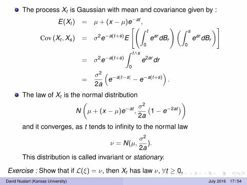
Proposition (Integration by parts formula)Let F ∈ S and let ut , t ∈ [0,T ] be an m-dimensional progressivelymeasurable process that satisfies Novikov condition. Then

E

(∫ T

0〈DsF ,us〉ds

)= E

(F∫ T

0usdBs

).


Proof :

(i) Let F = f (∫ T

0 h1sdBs, . . . ,

∫ T0 hn

sdBs). Fix ε > 0 and write

Fε = f

(∫ T

0h1

sd(

Bs + ε

∫ s

0ur dr

), . . . ,

∫ T

0hn

sd(

Bs + ε

∫ s

0ur dr

)).

(ii) From Girsanov’s theorem, we have

E [Fε] = E

(exp

(ε

∫ T

0ur dBs −

ε2

2

∫ T

0u2

r dr

)F

),

which implies

limε→0

1ε

(E [Fε]− E [F ]) = E

(F∫ T

0usdBs

).


(iii) On the other hand,

limε→0

1ε

(E [Fε]− E [F ])

= E

(∫ T

0

n∑i=1

∂f∂xi

(∫ T

0h1

sdBs, . . . ,

∫ T

0hn

sdBs

)〈hi

s,us〉ds

)

= E

(∫ T

0〈DsF ,us〉ds

).


For any p ≥ 1 we denote by LpT the space of d-dimensional measurable

processes Xt , t ∈ [0,T ] such that

E

(∫ T

0‖Xt‖2dt

) p2 <∞.

PropositionThe operator D is closable from Lp(Ω,FT ,P) into Lp

T , for any p ≥ 1.


Proof in the case p > 1 :

(i) Let Fn ∈ S, FnLp

→ 0 and such that DFnLp

T→ X . We claim that X = 0.

(ii) For any h ∈ L2([0,T ];Rd ) and G ∈ S, we have

limn→∞

E

(∫ T

0G〈DsFn,hs〉ds

)= E

(G∫ T

0〈Xs,hs〉ds

)and

E

(∫ T

0G〈DsFn,hs〉ds

)= E

(∫ T

0〈Ds(GFn),hs〉ds

)

−E

(∫ T

0Fn〈DsG,hs〉ds

)

= E

(Fn

[G∫ T

0hsdBs −

∫ T

0〈DsG,hs〉ds

])→ 0.

As a consequence, we obtain E(

G∫ T

0 〈Xs,hs〉ds)

= 0, which impliesX = 0.


The domain of D, denoted by D1,p is the closure of S under the norm

‖F‖1,p =(

E(|F |p) + E(‖DF‖pL2([0,T ];Rd )

) 1p.

For p > 1 we can consider the adjoint operator δ of D. It is a denselydefined operator from Lp

T into Lp(Ω,FT ,P), characterized by the dualityrelation

E(Fδ(u)) = E

(F∫ T

0usdBs

), F ∈ D1,p.

The domain of δ in LpT contains the space of d-dimensional

progressively measurable processes u in LpT and

δ(u) =

∫ T

0usdBs.


Clark-Ocone formiula

Proposition

Let F ∈ D1,2. Then,

F = E(F ) +

∫ T

0E(DtF |Ft )dBt .


Proof :

Assume d = 1. For any v ∈ L2(P) we can write, using the dualityrelationship

E

(F∫ T

0vtdBt

)= E(Fδ(v)) = E

(∫ T

0DtFvtdt

)

=

∫ T

0E [E(DtF |Ft )vt ]dt .

If we assume that F = E(F ) +∫ T

0 utdBt , then by the Ito isometry

E

(F∫ T

0vtdBt

)=

∫ T

0E(utvt )dt .

Comparing these two expressions we deduce that

ut = E(DtF |Ft )

almost everywhere in Ω× [0,T ].


If F ∈ S, the k th derivative of F is the k -parameter process with valuesin Rd×k given by

Dkt1,...,tk F = Dt1 · · ·Dtk F .

For any p ≥ 1 the operator Dk is closable on S. We denote by Dk,p theclosure of S with respect to the norm

‖F‖k,p =

E [|F |p] +k∑

j=1

E(‖DF‖pL2([0,T ]j ;Rd )

)

1p

.

SetD∞ = ∩p≥1 ∩k≥1 Dk,p.


Existence and regularity of densities

Let F = (F 1, . . . ,F m) be such that F i ∈ D1,2 for i = 1, . . . ,m.

The Malliavin matrix of F is

γF = (〈DF i ,DF j〉L2([0,T ];Rd ))1≤i,j≤m.

Theorem (Criterion for absolute continuity)If det γF > 0 a.s., then the law of F is absolutely continuous with respect tothe Lebesgue measure on Rm.

Theorem (Criterion for smoothness of the density)If Fi ∈ D∞ and E [(det γF )−p] <∞ for all p ≥ 1, then the law of F possessesand infinitely differentiability density.


Let F = Xt , where Xt , t ≥ 0 is the diffusion process on Rm

dXt = b(Xt )dt +d∑

k=1

σk (Xt )dBkt , X0 = x0.

TheoremIf the Lie algebra spanned by σ1, . . . , σd at x = x0 is Rm, whereσk =

∑mi=1 σik

∂∂xi

, then for any t > 0 (det γXt )−1 ∈ ∩p≥2Lp(Ω) and the density

pt (x) of Xt is C∞.

pt (x) satisfies the Fokker-Planck equation(− ∂

∂t+ L∗

)pt = 0,

where

L =12

m∑i,j=1

(σσT )ij∂2

∂xi∂xj+

m∑i=1

bi∂

∂xi.

Then, pt ∈ C∞ means that ∂∂t −L∗ is hypoelliptic (Hormander’s theorem).


References :

1 F. Baudoin : Diffusion Processes and Stochastic Calculus. EMS,2010.

2 I. Karatzas and S. E. Shreve : Brownian Motion and StochasticCalculus. Springer, 1998.

3 D. Nualart : Lecture Notes on Stochastic Processes.4 D. Nualart : The Malliavin calculus and related topics. Springer,

2005.


Lecture 3: Stochastic Differential Equations › ~song › Gene Golub Summer... · Linear stochastic differential equations The geometric Brownian motion X t = ˘e ˙ 2 2 t+˙Bt solves

Documents