1 Business Statistics Lecture 3: Random Variables and the Normal Distribution

Welcome message from author
This document is posted to help you gain knowledge. Please leave a comment to let me know what you think about it! Share it to your friends and learn new things together.
Transcript
1
Business Statistics
Lecture 3: Random Variables and the
Normal Distribution

2
• A little bit of probability
• Random variables
• The normal distribution
Goals for this Lecture
3
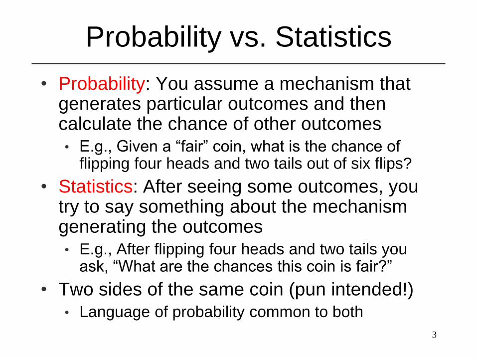
Probability vs. Statistics
• Probability: You assume a mechanism that generates particular outcomes and then calculate the chance of other outcomes• E.g., Given a “fair” coin, what is the chance of
flipping four heads and two tails out of six flips?
• Statistics: After seeing some outcomes, you try to say something about the mechanism generating the outcomes• E.g., After flipping four heads and two tails you
ask, “What are the chances this coin is fair?”
• Two sides of the same coin (pun intended!)• Language of probability common to both

4
Definitions
• Sample space (S)
• Set of all possible
outcomes of an experiment
• Event
• Collection of one or more
outcomes
• Probability
• Function assigning a
number from 0 to 1 to
events, subject to rules
S
AS
Venn Diagrams

5
Examples:
Sample Spaces and Events
• Roll a fair die: S = {1,2,3,4,5,6}
• Simple events
• Roll is a 1
• Roll is a 6
• Compound event
• Roll is even: {2, 4, 6}
• Roll is less than 4: {1, 2, 3}
• Fair: each simple event is equally likely
• Other sample space examples:
• Flip of one coin: S = {H, T}
• Flip two coins: S = {(H,H), (H,T), (T,H), (T,T)}
6
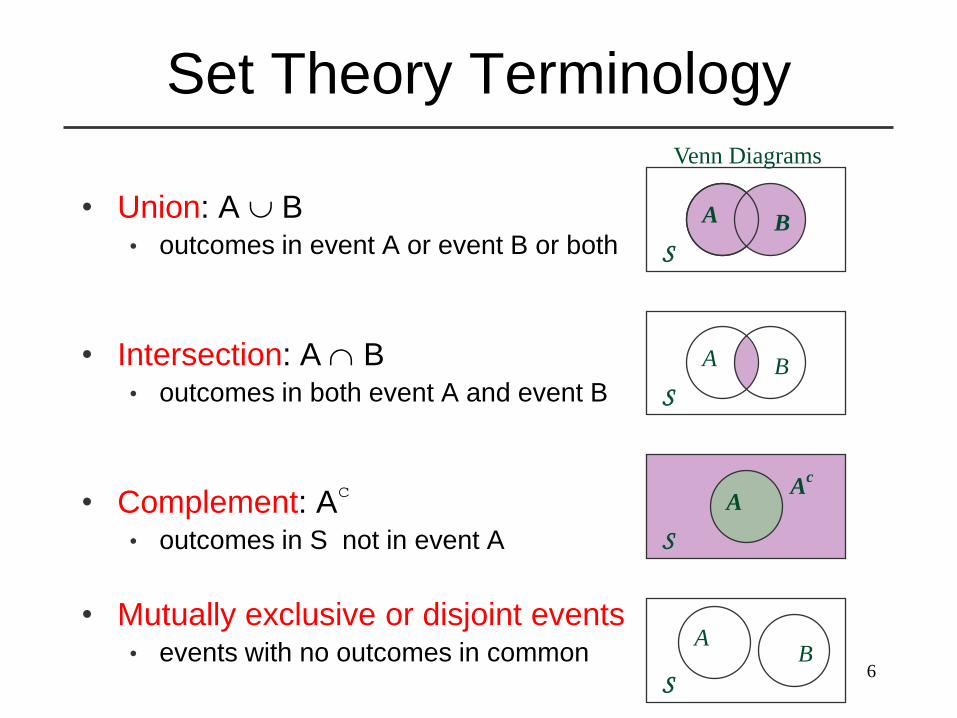
Set Theory Terminology
• Union: A B• outcomes in event A or event B or both
• Intersection: A B• outcomes in both event A and event B
• Complement: Ac
• outcomes in S not in event A
• Mutually exclusive or disjoint events• events with no outcomes in common
S
A B
S
AB
S
A B
S
A
Venn Diagrams
Ac
7
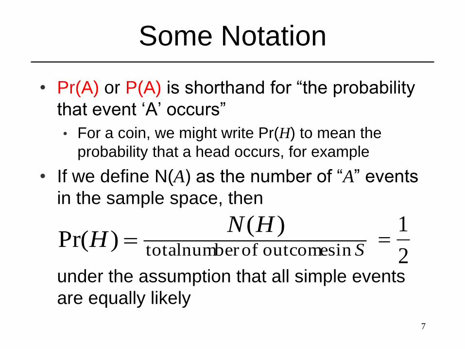
Some Notation
• Pr(A) or P(A) is shorthand for “the probability
that event „A‟ occurs”
• For a coin, we might write Pr(H) to mean the
probability that a head occurs, for example
• If we define N(A) as the number of “A” events
in the sample space, then
under the assumption that all simple events
are equally likely
S
HNH
in outcomes ofnumber total
)()Pr(
2
1
8
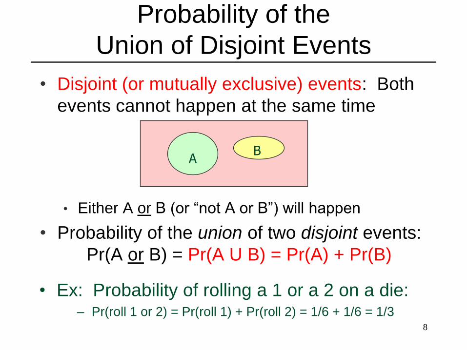
• Disjoint (or mutually exclusive) events: Both
events cannot happen at the same time
• Either A or B (or “not A or B”) will happen
• Probability of the union of two disjoint events:
Pr(A or B) = Pr(A U B) = Pr(A) + Pr(B)
AB
• Ex: Probability of rolling a 1 or a 2 on a die:– Pr(roll 1 or 2) = Pr(roll 1) + Pr(roll 2) = 1/6 + 1/6 = 1/3
Probability of the
Union of Disjoint Events

9
General Rule for Probability of
the Union of Two Events
• Both events can happen at the same time
• Yellow/green striped region
• In general, probability of the union of two events:
Pr (A and b) = Pr(A U B) = Pr(A) + Pr(B) – Pr(A B)
• Pr(A B) is the intersection of A and B
• Basically, the striped area is counted twice in
Pr(A) + Pr(B), so one must be subtracted off
• When events are disjoint Pr(A B) = 0
AB
U
U
U

10
• Complementary events: Either one or
the other will happen, but not both
• Either A will happen or “not A” will happen
• Pr(not A) = Pr(Ac) = 1 - Pr(A)
ANot A
• Ex: The probability that you do not roll a 3 is
1 minus the probability that you roll a 3– Pr(not roll 3) = 1 – Pr(roll 3) = 1 – 1/6 = 5/6
Probability An Event
Will Not Happen

Probability of the Intersection of
Independent Events
• Independent events:
Two observations are
independent if knowing
the value of one doesn‟t help you guess the
value of the other
• Rule: Pr(A and B) = Pr(A B) = Pr(A) x Pr(B)
• Example: In two rolls, the probability you roll
a 1 both times
• Pr( roll a 1 both times)
= Pr(roll 1 on first roll) x Pr(roll 1 on second roll)
= 1/6 x 1/6 = 1/3611
AB
U
12
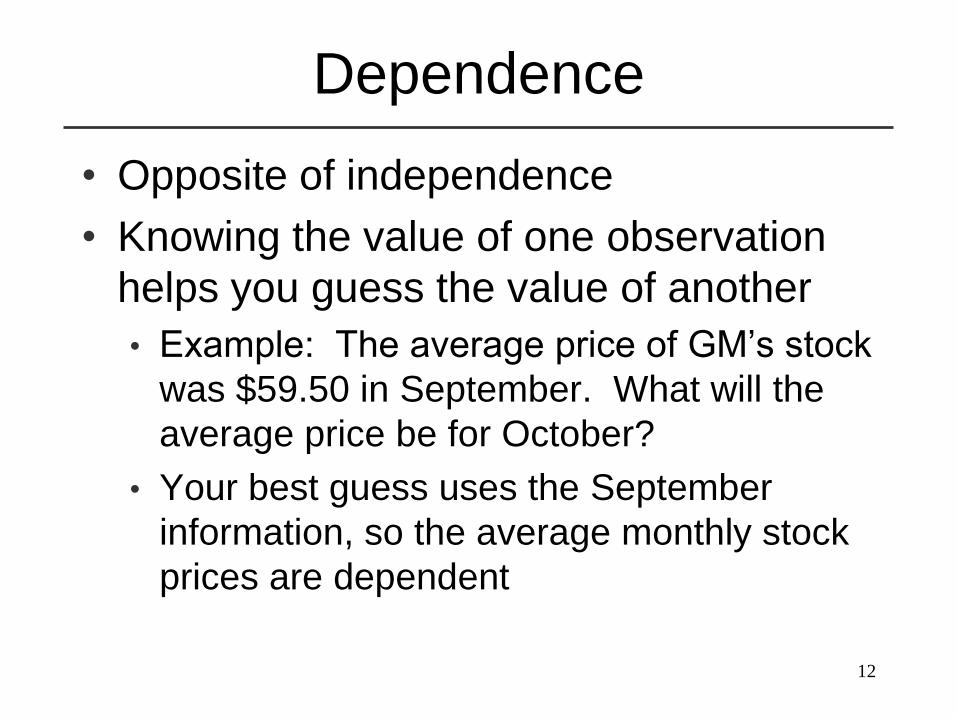
Dependence
• Opposite of independence
• Knowing the value of one observation
helps you guess the value of another
• Example: The average price of GM‟s stock
was $59.50 in September. What will the
average price be for October?
• Your best guess uses the September
information, so the average monthly stock
prices are dependent
13
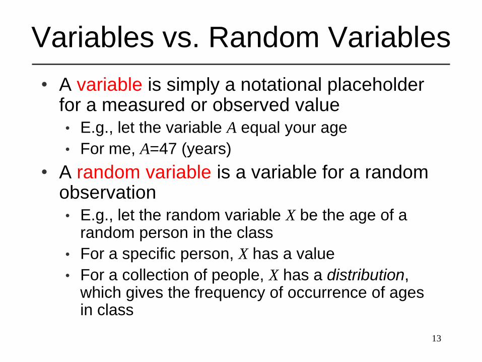
Variables vs. Random Variables
• A variable is simply a notational placeholder for a measured or observed value• E.g., let the variable A equal your age
• For me, A=47 (years)
• A random variable is a variable for a random observation• E.g., let the random variable X be the age of a
random person in the class
• For a specific person, X has a value
• For a collection of people, X has a distribution, which gives the frequency of occurrence of ages in class

14
Random Variables
• From the first class:
Let X be the outcome of a dice roll
• X is a random variable
• X can be equal to 1, 2, 3, 4, 5, or 6
depending on what occurs on the roll of a
dice
• X has a distribution:
• Probability X=x is 1/6, for x=1,2,3,4,5, or 6
• Notation: Pr(X=x)=1/6, for x=1,2,3,4,5, or 6

15
Plotting a Probability Distribution
• Let X denote the outcome of a fair die
• i.e., Pr(X=x)=1/6, for x=1,2,3,4,5, or 6
• We can draw the probability function:
Pr
(X=
x)
x
1/6
2/6
0 1 2 3 4 5 6
0
16
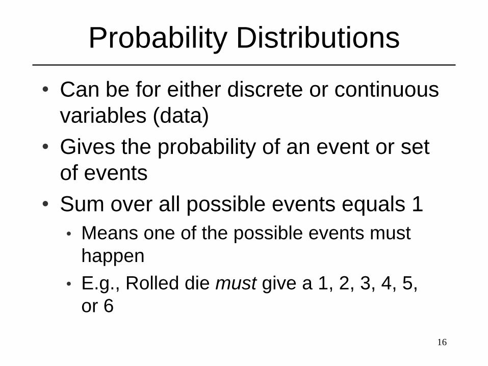
Probability Distributions
• Can be for either discrete or continuous
variables (data)
• Gives the probability of an event or set
of events
• Sum over all possible events equals 1
• Means one of the possible events must
happen
• E.g., Rolled die must give a 1, 2, 3, 4, 5,
or 6
17
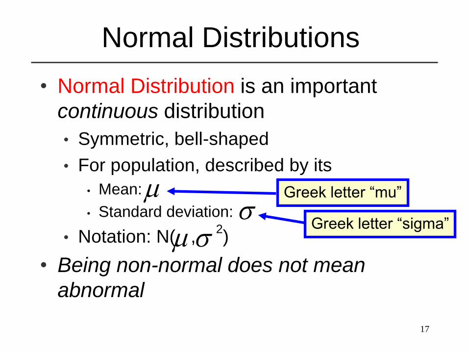
• Normal Distribution is an important
continuous distribution
• Symmetric, bell-shaped
• For population, described by its
• Mean:
• Standard deviation:
• Notation: N( , 2)
• Being non-normal does not mean
abnormal
Normal Distributions
Greek letter “mu”
Greek letter “sigma”
18
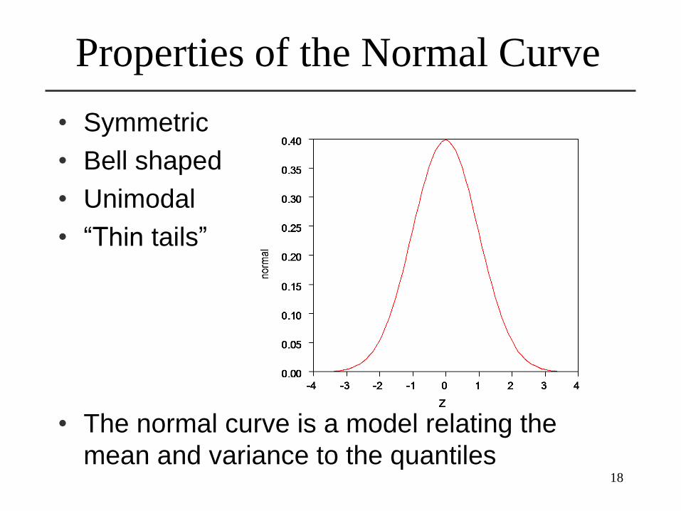
Properties of the Normal Curve
• Symmetric
• Bell shaped
• Unimodal
• “Thin tails”
• The normal curve is a model relating the
mean and variance to the quantiles
19
Why Focus on the
Normal Distribution?
• Normal distribution describes many
natural phenomenon well
• Central Limit Theorem explains why
• Statistical theorem: Distribution of sums of
random variables tends toward the normal
• The more things that are summed, the
more like the normal
• Result is that averages tend to have a
normal distribution

Central Limit Theorem in Action
.01
.05
.10
.25
.50
.75
.90
.95
.99
-3
-1
0
2
.0 .1 .2 .3 .4 .5 .6 .7 .8 .9 1.0
Hig
hly
skew
ed
pro
cess
.0 .1 .2 .3 .4 .5 .6 .7
.01
.05
.10
.25
.50
.75
.90
.95
.99
-3
-1
1
3
Mean of 5
•.01
•.05
•.10
•.25
•.50
•.75
•.90•.95
•.99
-3
-2
-1
0
1
2
3
.0 .1 .2 .3 .4 .5 .6
Mean of 10 .01
.05
.10
.25
.50
.75
.90
.95
.99
-3
-2
-1
0
1
2
3
.2 .3
Mean of 100
21
• A statistic is a one-number summary of data
• Statistics can be for samples or populations
• x-bar and s are examples of sample statistics
• and are parameters of the normal
distribution
• We often estimate parameters with statistics
• Estimate with
• Estimate with s
Statistics and Parameters
X

22
…has a corresponding
sample summary
• Mean
• Standard deviation
• Proportion
Statistics
x
s
p̂
Sample statistics are good guesses for
population parameters, but they’re not the
same
Parameters vs. Statistics
• Every population
summary…
• Mean ()
• Standard Deviation
()
• Proportion (p)
Parameters

23
The Empirical Rule
0.00
0.05
0.10
0.15
0.20
0.25
0.30
0.35
0.40
-4 -3 -2 -1 0 1 2 3 4
Z
• If the normal curve
fits well then:
99%
• 99% within 3 SD68%
• 68% of the data is
within 1 SD of the
mean
95%
• 95% within 2 SD
24
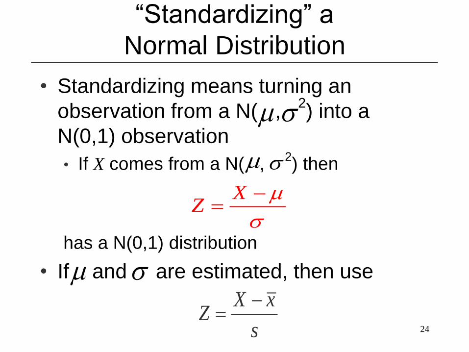
“Standardizing” a
Normal Distribution
• Standardizing means turning an
observation from a N( , 2) into a
N(0,1) observation
• If X comes from a N( , 2) then
has a N(0,1) distribution
• If and are estimated, then use
XZ
X x
Zs

25
• See Table A3-2 on page 491 in Business Statistics
• Enter with a value of “a”
• Read across to the “p” column to get probability of being between a and –a
• Example: a=1• Probability is 0.6827 of being between 1 and –1
• Empirical rule!
• Note: Can also go in the other direction to find the a-value corresponding to a probability
Finding the Probability
for a Normal Distribution (1)
26
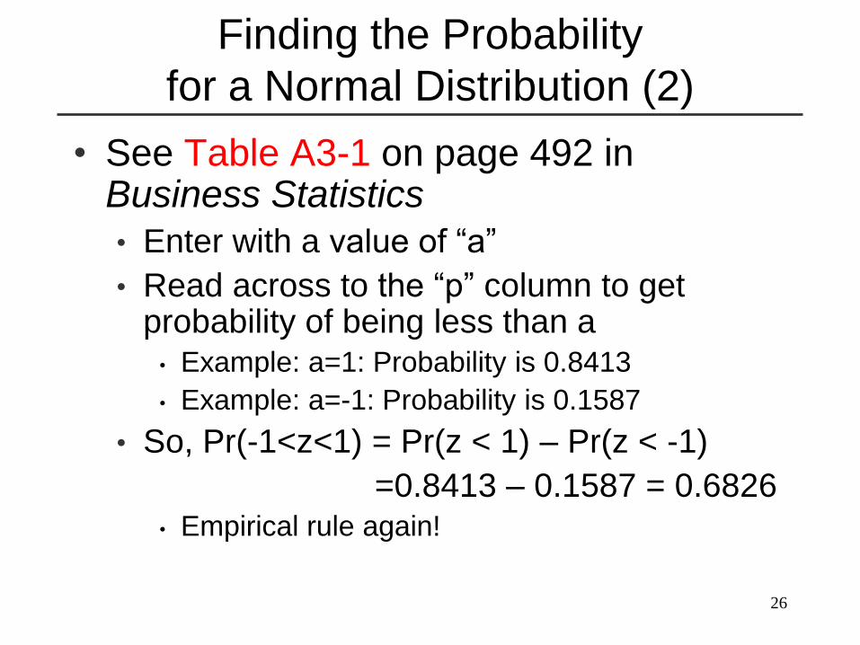
• See Table A3-1 on page 492 in Business Statistics
• Enter with a value of “a”
• Read across to the “p” column to get probability of being less than a
• Example: a=1: Probability is 0.8413
• Example: a=-1: Probability is 0.1587
• So, Pr(-1<z<1) = Pr(z < 1) – Pr(z < -1)
=0.8413 – 0.1587 = 0.6826• Empirical rule again!
Finding the Probability
for a Normal Distribution (2)
27
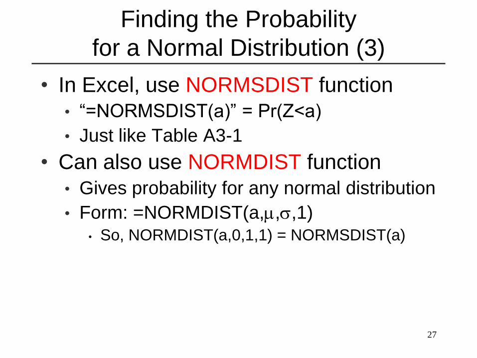
• In Excel, use NORMSDIST function
• “=NORMSDIST(a)” = Pr(Z<a)
• Just like Table A3-1
• Can also use NORMDIST function
• Gives probability for any normal distribution
• Form: =NORMDIST(a,,,1)• So, NORMDIST(a,0,1,1) = NORMSDIST(a)
Finding the Probability
for a Normal Distribution (3)

28
• For a standard normal distribution:
• What is the probability of being outside of the interval (3, -3)?
• What is the probability of getting an observation less than –2?
• For a N(1,32) distribution:
• What is the probability of being within one standard deviation of the mean?
• What is the probability of getting an observation greater than 7?
Exercises in finding the Probability
for a Normal Distribution
Solutions…
29
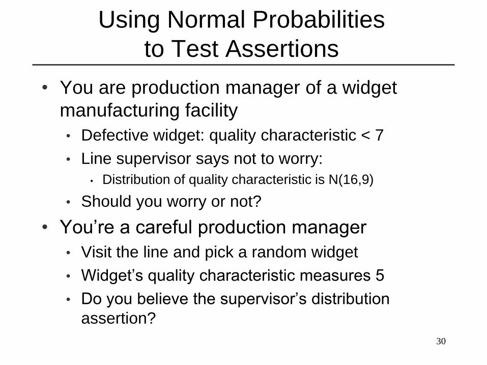
30
Using Normal Probabilities
to Test Assertions
• You are production manager of a widget
manufacturing facility
• Defective widget: quality characteristic < 7
• Line supervisor says not to worry:
• Distribution of quality characteristic is N(16,9)
• Should you worry or not?
• You‟re a careful production manager
• Visit the line and pick a random widget
• Widget‟s quality characteristic measures 5
• Do you believe the supervisor‟s distribution
assertion?
The Calculations…
31
32
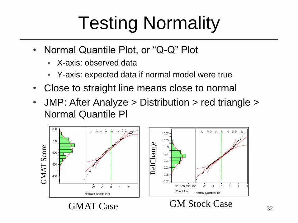
Testing Normality
• Normal Quantile Plot, or “Q-Q” Plot
• X-axis: observed data
• Y-axis: expected data if normal model were true
• Close to straight line means close to normal
• JMP: After Analyze > Distribution > red triangle >
Normal Quantile Pl
400
500
600
700
800.01 .05.10 .25 .50 .75 .90.95 .99
-2 -1 0 1 2 3
Normal Quantile Plot
GMAT Case
-0.07
-0.05
-0.03
-0.01
0.01
0.03
0.05
0.07
50 100 150 200
Count Axis
.01 .05.10 .25 .50 .75 .90.95 .99
-2 -1 0 1 2 3
Normal Quantile Plot
GM Stock Case
Rel
Chan
ge
GM
AT
Sco
re
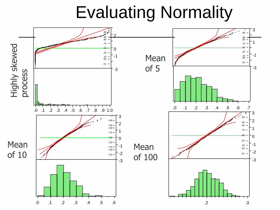
Evaluating Normality
.01
.05
.10
.25
.50
.75
.90
.95
.99
-3
-1
0
2
.0 .1 .2 .3 .4 .5 .6 .7 .8 .9 1.0
Hig
hly
skew
ed
pro
cess
.0 .1 .2 .3 .4 .5 .6 .7
.01
.05
.10
.25
.50
.75
.90
.95
.99
-3
-1
1
3
Mean of 5
•.01
•.05
•.10
•.25
•.50
•.75
•.90•.95
•.99
-3
-2
-1
0
1
2
3
.0 .1 .2 .3 .4 .5 .6
Mean of 10 .01
.05
.10
.25
.50
.75
.90
.95
.99
-3
-2
-1
0
1
2
3
.2 .3
Mean of 100
In the Readings…
• …don‟t worry too much about:
• Sampling with and without replacement
• Permutations and combinations
• Uniform, t, chi-square, and F distributions
• If we had more time, we‟d cover these
topics
34
35
What we have learned so far…
• Types of data and types of variation
• Descriptive statistics
• Statistical plots and graphs
• Random variables and a little probability
• “And,” “Or,” “Not” rules
• The normal distribution
• Standardizing
• Calculating probabilities
Related Documents