Lecture 3 Radiative and Convective Energy Transport I. Mechanisms of Energy Transport II. Radiative Transfer Equation III. Grey Atmospheres IV. Convective Energy Transport V. Mixing Length Theory

Lecture 3 Radiative and Convective Energy Transport
Jan 01, 2016
Lecture 3 Radiative and Convective Energy Transport. Mechanisms of Energy Transport Radiative Transfer Equation Grey Atmospheres Convective Energy Transport Mixing Length Theory. The Sun. I. Energy Transport. - PowerPoint PPT Presentation
Welcome message from author
This document is posted to help you gain knowledge. Please leave a comment to let me know what you think about it! Share it to your friends and learn new things together.
Transcript

Lecture 3Radiative and Convective Energy Transport
I. Mechanisms of Energy Transport
II. Radiative Transfer Equation
III. Grey Atmospheres
IV. Convective Energy Transport
V. Mixing Length Theory

The Sun

I. Energy Transport
In the absence of sinks and sources of energy in the stellar atmosphere, all the energy produced in the stellar interior is transported through the atmosphere into outer space. At any radius, r, in the atmosphere:
4r2F(r) = constant = L
Such an energy transport is sustained by the temperature gradient. The steepness of this gradient is in turn dependent on the effectiveness of the energy transport through the different layers

I. Mechanisms of Energy Transport
1. Radiation Frad (most important)
2. Convection: Fconv (important in cool stars like the Sun)
3. Heat production: e.g. in the transition between the solar chromosphere and corona
4. Radial flow of matter: coronae and stellar winds
5. Sound waves: chromosphere and coronae
Since we are dealing with the photosphere we are mostly concerned with 1) and 2)

I. Interaction between photons and matter
Absorption of radiation:
I IdI
s
dI= – I dx : mass absorption coefficient[ ] = cm2 gm–1
=∫0
s
dx Optical depth (dimensionless)
Convention: = 0 at the outer edge of the atmosphere, increasing inwards
d = ds

Optical Depth
I I(s)
dI= –I d → I(s) = Ie–
The intensity decreases exponentially with path length
Optically thick: > 1
Optically thin: < 1
If = 1 → =Ie
≈ 0.37 I0
We can see through the atmosphere until ~1


Optical depth, , of ring material small
Optical path length small and you see central star and little nebular material
Optical path length larger and you see nebular material as ring
Optical depth, , of ring material larger
Optical path length roughly the same one sees disk and no central star

Optical Depth
The quantity = 1 has a geometrical interpretation in terms of the mean free path of a photon:
= 1 = ∫ ds = s
s ≈ ()–1
s is the distance a photon will travel before it gets absorbed. In the stellar atmosphere the abosrbed will get re-emitted and thus will undergo a „random walk“. For a random walk the distance traveled in 1-D is s√N where N is the number of encounters. In 3-D the
number of steps to go a distance R is 3R2/s2.
s At half the solar radius ≈ 2.5 thus s ≈ 0.4cm so it takes ≈ 30.000 years for a photon do diffuse outward from the core of the sun.

Emission of Radiation
II+ dI
dxj
dI= j I dx
jis the emission coefficient/unit mass
[ ] = erg/(s rad2 Hz gm)
j comes from real emission (photon created) or from scattering of photons into the direction considered.

II. The Radiative Transfer Equation
Consider radiation traveling in a direction s. The change in the specific intensity, I, over an increment of the path length, ds, is just the sum of the losses () and the gains (j) of photons:
dI= – I j I ds
Dividing by ds which is just d
= –I j/ = –I + S
dI
d
The Radiative Transfer Equation
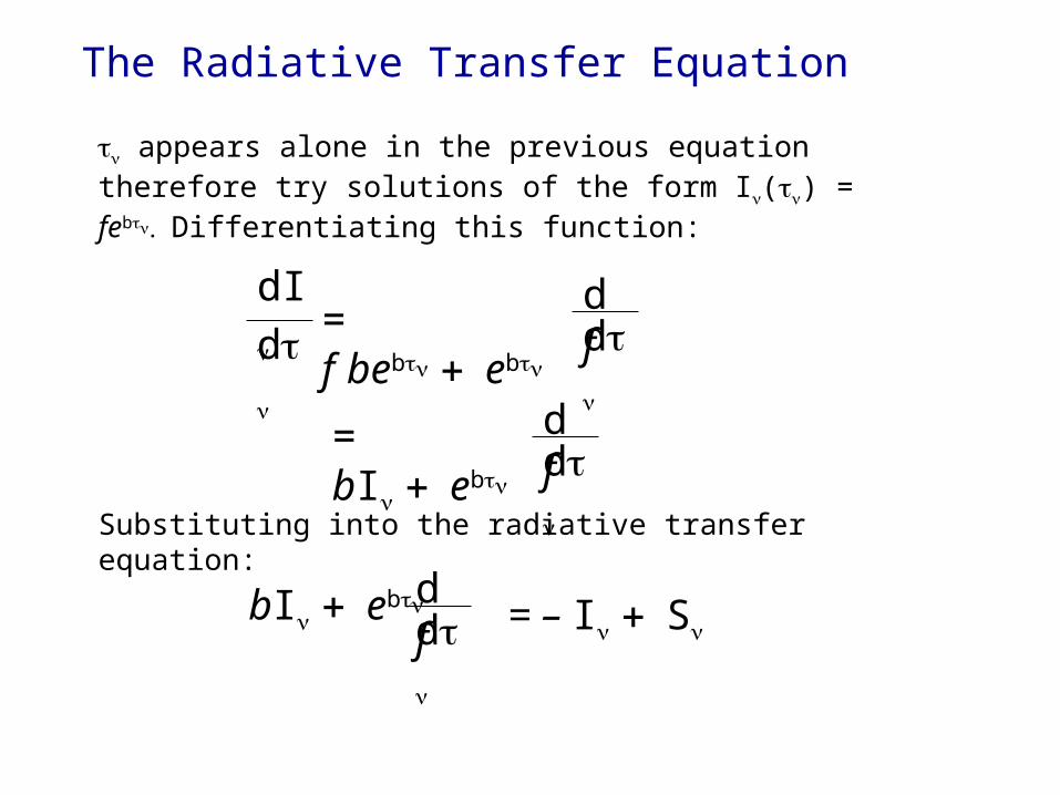
appears alone in the previous equation therefore try solutions of the form I() = febDifferentiating this function:
= fbebeb
dI
d
dfd
= bI
eb
dfd
Substituting into the radiative transfer equation:
bIeb df
d= – IS

The Radiative Transfer Equation
The first two terms on each side are equal if we set b = –1 and equating the second term:
e–dfd
or
= S
f = ∫ Setdt + c00
t is a dummy variable
I() = feb =e–∫S(t)et dt+ c0e–
0
Set = 0 → c0 = I(0)

bringing e– inside the integral:
I() =∫S(t)e–(–t + Ie–
0
=0
I(0)→
t
–t
At point tn the original intensity, I(0) suffers an exponential extinction of e–
The intensity generated at t, S(t) undergoes an extinction of e–(–t) before being summed at point

I() =∫S(t)e–(–t + Ie–
0
This equation is the basic intergral form of the radiative transfer equation. To perform the integration, S(), must be a known function. In some situations this is a complicated function, other times it is simple. In the case of thermodynamic equilibrium (LTE),
S(T) = B(T), the Planck function. Knowing T as a function of x or amounts to a solution of the transfer equation.

Radiative Transfer Equation for Spherical Geometry
After all, stars are spheres!
z
x
y
To observer
dz
r
dr
rd
dIdz = –I + S
dIdz
= ∂I∂z
drdz
∂I∂
ddz+

Radiative Transfer Equation for Spherical Geometry
Assume I has nodependence and
dr = cos dz
r d = –sin
∂I
∂rcos dr
–∂I
∂sin r
= –I + S
This form of the equation is used in stellar interiors and the calculation of very thick stellar atmospheres such as supergiants. In many stars (sun) the photosphere is thin thus we can use the plane parallel approximation

Plane Parallel ApproximationTo observer
ds
To center of star
does not depend on z so there is no second term
dIcos dr= –I + S
Custom to adopt a new depth variable x defined by dx = –dr. Writing d for dx:
dIcos d
= I – S
The increment of path length along the line of sight is ds = dx sec

The optical depth is measured along x and not along the line of sight which is at some angle . Need to replace by –sec The negative sign arises from choosing dx = –dr
c
Therefore the radiative transfer equation becomes:
I() =–∫S(t)e–(t–sec sec d
The integration limit c replaces I(0) integration constant because the boundary conditions are different for radiation going in ( > 90o) and coming out ( < 90o).
In the first case we start at the boundary where =0 and work inwards. So when I = I
in, c=0.
In the second case we consider radiation at the depth and deeper until no more radiation can be seen coming out. When I=Iout, c=∞

Therefore the full intensity at the position on the line of sight through the photosphere is:
I()
= ∫Se–(t–sec sec dt∞
= Iout() + I
in() =
– ∫Se–(t–sec sec dt0
Note that one must require that Se–goes to zero as goes to infinity. Stars obviously can do this!

An important case of this equation occurs at the stellar surface:
Iin() = 0
Iout() = ∫S(t)e–tsec sec dt
∞
Assumption: Ignore radiation from the rest of the universe (other stars, galaxies, etc.)
This is what you need to compute a spectrum. For the sun which is resolved, intensity measurements can be made as a function of . For stars we must integrate I over the disk since we
observe the flux.

The Flux Integral
∫ Icosd
F=
∫ Icossin dF= 2
= ∫ Ioutcossin
d
2
+ ∫ Iincossin
d
2
Assuming no azimuthal () dependence

The Flux Integral
Using previous definitions of Iin and I
out
∫F= 2
∫
∞
Se–(t–sec sin dtd
∫– 2
∫
0
Se–(t–sec sin dtd

The Flux Integral
If S is isotropic
– 2 ∫
∫
e–(t–sec sin dtd S
Let w = sec and x = t –
F= 2 ∫
∫
∞
e–(t–sec sin dtd S
∫
e–(t–sec sin dtd ∫∞
e–xw
w2dw
=

The Flux Integral
∫∞
e–xw
wndw
Exponential Integrals
En(x) =
F= 2 ∫
∞
SE2t– )dt– 2 ∫
0
SE2– t)dt
In the second integral w = –sec and x = – t. The limit as goes from /2 to is approached with negative values of cos so w goes to ∞ not –∞

The Flux Integral
The theoretical spectrum is F at = 0:
F= 2 ∫
∞
StE2t)dtF is defined per unit area
In deriving this it was assumed that S is isotropic. It most instances this is a reasonable assumption. However, in stars there are Doppler shifts due to photospheric velocities, stellar rotation, etc. Isotropy no longer holds so you need to do an explicit disk integration over the stellar surface, i.e. treat F locally and add up all contributions.

The Mean Intensity and K Integrals
J= 1/2∫
∞
SE1t– )dt+ 1/2
∫
0
SE1– t)dt
K= 1/2
∫
∞
SE3t– )dt+ 1/2
∫
0
SE3– t)dt

The Exponential Integrals
∫∞
e–xw
wndw
Exponential Integrals
En(x) =
∫∞
wn
dwEn(0) = =1–n1
∫∞
e–xw
wn dwdEn
dx =1 d
dx ∫∞
e–xw
wn–1dw= –
dEn
dx = –En–1

The Exponential Integrals
Recurrence formula
En+1(x) = e–x –xEn(x)

The Exponential Integrals
For computer calculations:
E1(x) = e–x –xEn(x)
E1(x) = –ln x – 0.57721566 + 0.99999193x – 0.24991055x2 + 0.05519968 x3 – 0.00976004x4 + 0.00107857x5 for
x ≤ 1
E1(x) = x4 + a3x3 + a2x2 + a1x + a0
x4 + b3x3 + b2x2 + b1x + b0
1xex
a3 = 8.5733287401
a2= 18.0590169730
a1= 8.6347608925
a0= 0.2677737343
b3= 9.5733223454
b2= 25.6329561486
b1= 21.0996530827
b0= 3.9584969228
En(x) =1
xex [1 – nx
n(n+1)x2
+ – … [
xex
1≈
Assymptotic Limit:
x >1
From Abramowitz and Stegun (1964)
Polynomials fit E1 to an error less than 2 x 10⁻⁷

Radiative Equilibrium
• Radiative equilibrium is an expression of conservation of energy
• In computing theoretical models it must be enforced
• Conservation of energy applies to the flow of energy through the atmosphere. If there are no sources or sinks of energy in the atmosphere the energy generated in the core flows to the outer boundary
• No sources or sinks in the atmosphere implies that the divergence of the flux is zero everywhere in the photosphere.
In plane parallel geometry:
ddx F(x) = 0 or F(x) = F0
A constant
F(x) = ∫F0 ()d=F0 for flux carried by radiation 0
∞

d ∫
∞
SE2t– )dt – ∫
0
SE2– t)dt
Radiative Equilibrium
∫
∞
[
[
=F0
2
This is Milne‘s second equation
It says that in the case of radiative equilibrium the solution of the radiative transfer equation is found when S is known that
satisfies this equation.

Radiative Equilibrium
Other two radiative equilibrium conditions come from the transfer equation :
dIcos dx
= I – S
Integrate over solid angle
ddx ∫ Icosd
= Id – Sd
∫ ∫Substitue the definitions of flux and mean intensity in the first and second integrals
dF
dx= 4J – 4S

Radiative Equilibrium
Integrating over frequency
But in radiative equilibrium the left side is zero!
ddx ∫
∞
Fd = 4Jd – 4Sd
∫
∞
∫
∞
∫
∞
Jd = ∫
∞
Sd
Note: the value of the flux constant does not appear

Radiative Equilibrium
Using expression for J
∫
∞
∫
∞
J= ½ ∫
∞
SE1t– )dt+ ½ ∫
0
SE1– t)dt
[½ = 0 SE1t– )dt ∫
0
SE1– t)dt+ ½
[d
First Milne equation

If you multiply radiative equation by cos you get the K-integral
dIcos2 dx
I cos – Scos
d dK = d
F0 ∫
∞1st moment2nd moment
∫ ∫=
4
dd
Radiative Equilibrium
∫
∞
∫
∞
[½ SE3t– )dt ∫
0
SE3– t)dt+ ½
[
d d
d=
F0
4
Third Milne Equation
And integrate over frequency

Radiative Equilibrium
The Milne equations are not independent. S that is a solution for one is a solution for all three
The flux constant F0 is often expressed in terms of an effective temperature, F0 = T4. The effective temperature is a fundamental parameter characterizing the model.
In the theory of stellar atmospheres much of the technical effort goes into iterative schemes using Milne‘s equations of radiative equilibrium to find the source function, S()

III. The Grey Atmosphere
The simplest solution to the radiative transfer equation is to assume that is independent of frequency, hence the name „grey“. It occupies an „historic“ place and is the starting point in many iterative calculations. Electron scattering is the only opacity source relevant to stellar atmospheres that is independent of frequency.
Integrate the basic transfer equation over frequency and denote:
I = ∫Id0
∞
J = ∫Jd0
∞
S = ∫Sd0
∞
K = ∫Kd0
∞
F = ∫Fd0
∞
dIcos d
= –I + S Where d = dx, the „grey“ absorption coefficient

The Grey Atmosphere
This grey case simplifies the radiative equilibrium and Milne‘s equations:
F(x) = F0
J = S
dKd
=F0
4
The Eddington approximation, hemispherically isotropic outward and inward specific intensity:
I() =Iout() for 0 ≤ ≤ /2
Iin() for ≤ ≤

The Grey Atmosphere
J = 1
4 ∫ Id = 12 ∫Iout
0
/2
sin d + 12 ∫Iin
/2
sin d
= 12
Iout () + Iin()
F() = Iout () – Iin()
K() = 16
Iout () + Iin()
S() = J() = 3K()
But since the mean intensity equals the source function in this case

The Grey Atmosphere
We can now integrate the equation for K:
K() = F0
4
F0
6
Where the constant is evaluated at = 0. Since S = 3K we get Eddington‘s solution for the grey case:
S() =3F0
4( + ⅔)
The source function varies linearly with optical depth. One gets a similar result from more rigorous solutions
dKd
=F0
4

III. The Grey Atmosphere
Using the frequency integrated form of Planck‘s law: S() = ()T4() and F0 = T4 the previous equation becomes
T() = ( + ⅔)¾¼
At = ⅔ the temperature is equal to the effective temperature and T() scales in proportion to the effective temperature.
Teff
Note that F(0) = S(⅔), i.e. the surface flux is times the source function at an optical depth of ⅔.

III. The Grey Atmosphere
Chandrasekhar (1957) gave a complete and rigorous solution of the grey case which is slightly different:
S() =3F0
4[ + q()]
T() = [ + q()]¾¼Teff
q() is a slowly varying function ranging from 0.577 at = 0 and 0.710 at = ∞
Eddington:
„This, however is a lazy way of handling the problem and it is not surprising that the result fails to accord with observation. The proper course is to find the spectral distribution of the emergent radiation by treating each wavelength separately using its own proper values of j and .“

IV. Convection
In a star the heat flux must be sufficiently great to transport all the energy that is liberated. This requires a temperature gradient. The higher the energy flux, the larger the temperature gradient. But the temperature gradient cannot increase without limits. At some point instability sets in and you get convetion
In hot stars (O,B,A) radiative transport is more efficient in the atmosphere, but core is convective.
In cool stars (F and later) convective transport dominates in atmosphere. Stars have an outer convection zone.


IV. Convection
T
r
1
*
P*
P
*
P*
2 P
Consider a parcel of gas that is perturbed upwards. Before the perturbation 1* = 1 and P1* = P1
For adiabatic expansion:
P = = CP/CV = 5/3Cp, Cv = specific heats at constant V, P
After the perturbation:
P2 = P2* 2* = 1(P2*
P1*)
1/

IV. Convection
Stability Criterion:
Stable: 2* > 2 The parcel is denser than its surroundings and gravity will move it back down.
Unstable: 2* < 2 the parcel is less dense than its surroundings and the buoyancy force will cause it to rise higher.

IV. Convection
Stability Criterion:
2*1
= ( P2
P1)
1/= {P1 +
dPdr r}
P1
1/
={ }1/
1 + r1P
dPdr
2* = 1 + (1
P )1 dPdr
r
2 = 1 +ddr r
(1
P )1 dPdr
ddr
>
This is the Schwarzschild criterion for stability

IV. Convection
By differentiating the logarithm of P =
k T we can relate
the density gradient to the pressure and temperature gradient:
( T
P)1dT
dr (1 – ) ( )dPdrstar
>star
The left hand side is the absolute amount of the temperature gradient of the star. Both gradients are negative, so this is the algebraic condition for stability. The right hand side is the „adiabatic temperature gradient“. If the actual temperature gradient exceeds the adiabatic temperature gradient the layer is unstable and convection sets in:
( )dT
dr ( )dTdrstar
<ad
The difference in these two gradients is often referred to as the „Super Adiabatic Temperature Gradient“

Brunt-Väisälä Frequency
The frequency at which a bubble of gas may oscillate vertically with gravity the restoring force:
The Convection Criterion is related to gravity mode oscillations:
is the ratio of specific heats = Cv/Cp
g is the gravity
( )1 dlnPdr
dlndr
–N2 = g
Where does this come from?

T
r
1
*
P*
P
*
P*
2 P
2* = 1 + (1
P )1 dPdr
r
2 = 1 +ddr r
Difference in density between inside the parcel and outside the parcel:
= (
P )1 dPdr
r –ddr r
= ( )1 dlnPdr
rdlndr r–
= ( )dlnP
drr dr r–1 dln
The Brunt-Väisälä Frequency

= Ar
= ( )dlnPdr dr–
1 dlnA
Buoyancy force:
FB = –Vg V = volume
FB = –gAVr
In our case x = r, k = gAV, m ~ V
( )dlnP dlnN2 = gAV/V = gA = g dr dr–
1
The Brunt-Väisälä Frequency is the just the harmonic oscillator frequency of a parcel of gas due to buoyancy
FB = –kx 2 = k/mFor a harmonic oscillator:

V. Mixing Length Theory
Convection is a difficult problem for which we still have no good theory. So how do most atmospheric models handle this complicated problem? By reducing it to a single free parameter whose value is left to guess work. This is mixing length theory. Physically it is a piece of junk, but at this point there is no alternative although progress has been made in hydrodynamic modeling.Simple approach:
1. Suppose the atmosphere becomes unstable at r = r0 → mass element rises for a characteristic distance L (mixing length) to r + L
2. Cell releases excess energy to the ambient medium
3. The cell cools, sinks back, absorbs energy and rises again
In this process the temperature gradient becomes shallower than in the purely radiative case.

V. Mixing Length Theory
Recall the pressure scale height:
H = kT/g
The mixing length parameter is given by
=LH
= 0.5 – 1.5

V. Mixing Length Theory
½v2 = gL = gH
The convective flux is given by:
= CpvT v is the convective velocity
= → v ≈ g½(H)½(½
= Cp T3/2gH
½
= Cp
g
½H) –d
dxcell
ddx
average
3/2
Or in terms of the temperature gradients

Scale height H = kT/g
The Sun: H~ 200 km
A red giant: H ~ 108 km
How large are the convection cells? Use the scale height to estimate this:

Schwarzschild (1976)
Schwarzschild argued that the size of the convection cell was roughly the width of the superadiabatic temperature gradient like seen in the sun.

In red giants this has a width of 107 km

Convective Cells on the Sun and Betelgeuse
Betelgeuse = Ori
From computer hydrodynamic simulations
The Sun
1000 km~107 km


Numerical Simulations of Convection in Stars:
http://www.astro.uu.se/~bf/movie/movie.html


http://www.aip.de/groups/sternphysik/stp/box_simulation.html
With no rotation: With rotation:

• cells small• large total number on surface• motions and temperature differences relatively small• Time scales short (minutes)• Relatively small effect on integrated light and velocity measurements
• cells large• small total number on surface• motions and temperature differences relatively large• Time scales long (years)• large effcect on integrated light and velocity measurements

RV Measurements from McDonald
AVVSO Light Curve
Related Documents


