Lecture 3 Population, income and resource constraints.

Lecture 3

Population, income and resource constraints.

Resource constraints and long run growth

• The first lecture pointed out that population decline was associated with economic decline and

• that population increase after the 9th century triggered off division of labour and economic growth

• What happens in the very long run if land is in limited supply?

Major issues confronted today

• What determines the long run demographic trends?

• Why has fertility declined in the modern world?

• Why do poor people have more kids than rich?

• Can economies grow for ever with limited resources such as a constant supply of land?

Economists used to say: No Way!

• For Malthus and Ricardo land was the limiting resource.

• For late 19th century economists coal was supposed to bring economic growth to a halt.

• Quite a few today argue that oil shortage will end prosperity and Malthus still has a big fan club.

The Malthus-Ricardo view

• Growth is constrained by limited resources, primarily land

• Population growth positively related to income per capita

• Technological progress is insignificant.• Population growth will depress real wages

in the long run because of diminishing returns and lead to population stagnation.

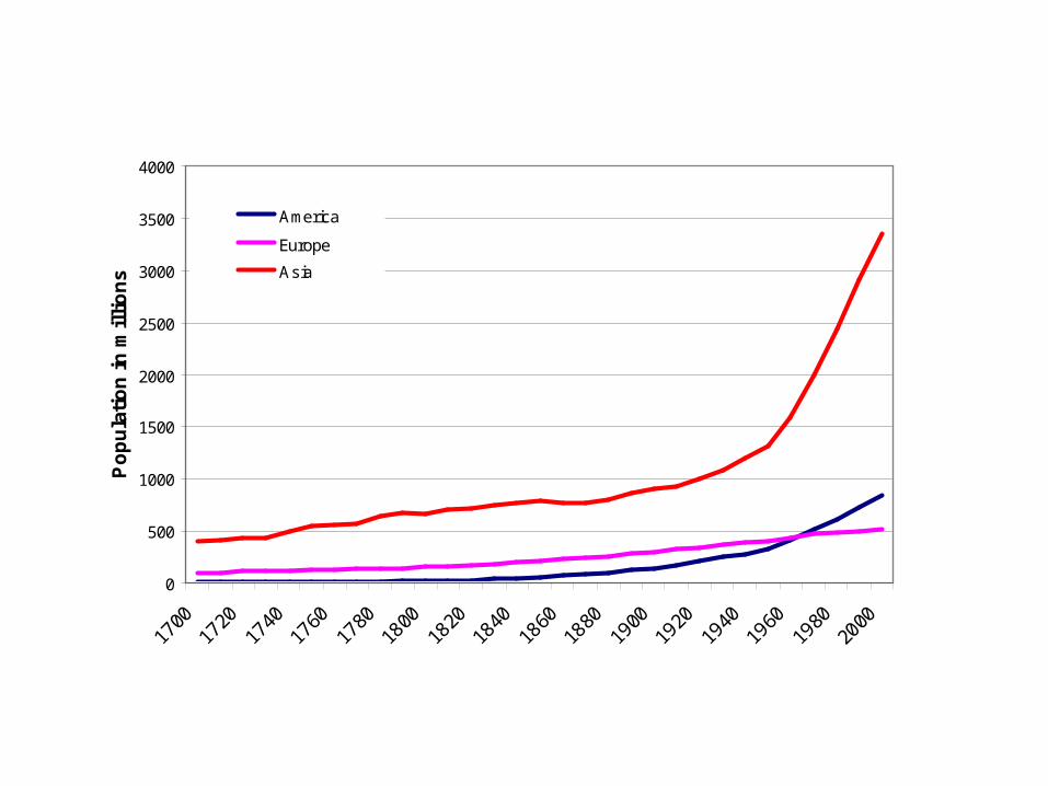
Malthus was wrong about the future

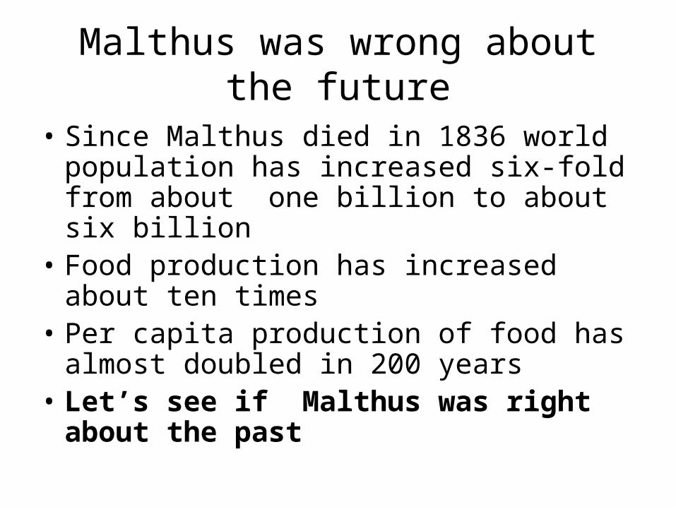
• Since Malthus died in 1836 world population has increased six-fold from about one billion to about six billion

• Food production has increased about ten times

• Per capita production of food has almost doubled in 200 years

• Let’s see if Malthus was right about the past

Some definitions

• cbr means crude birth rates and is usually measured as births per 1000

• cdr means crude death rates and is measured as deaths per 1000

• The rate of population growth = cbr – cdr

• cbr has an estimated maximum of 50 but it has rarely been observed historically

Malthusian population theory

Vital Rates

Income per headMalthusian EquilibriumCBR-CDR=0Income= Subsistence Constant population

CDR

CBR

The historical record suggests: Constant, above subsistence, income and positive population growth.

Preventive and positive checks

• The upward sloping cbr curve can be explained by the fact that preventive checks increase with falling income and vice versa: late marriages=less children.

• The downward slope of the cdr curve is due to that positive checks – increasing mortality – are triggered off by lower income: poor nutrional status=high risk for diseases.

Population growth with constant land

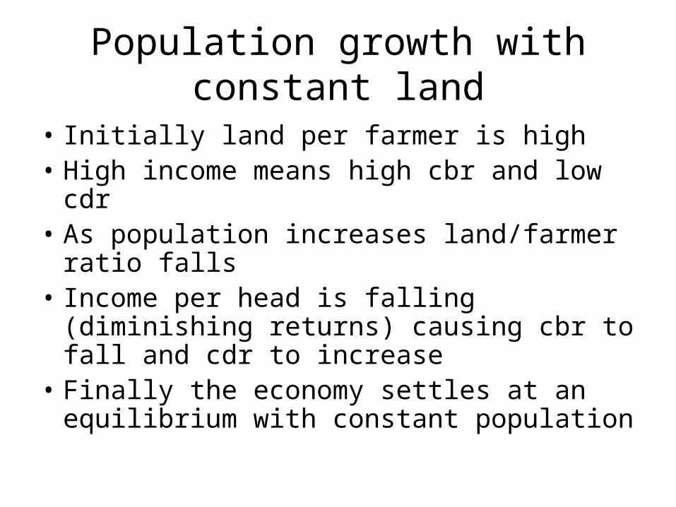
• Initially land per farmer is high• High income means high cbr and low cdr• As population increases land/farmer ratio

falls• Income per head is falling (diminishing

returns) causing cbr to fall and cdr to increase

• Finally the economy settles at an equilibrium with constant population

Malthus or climate

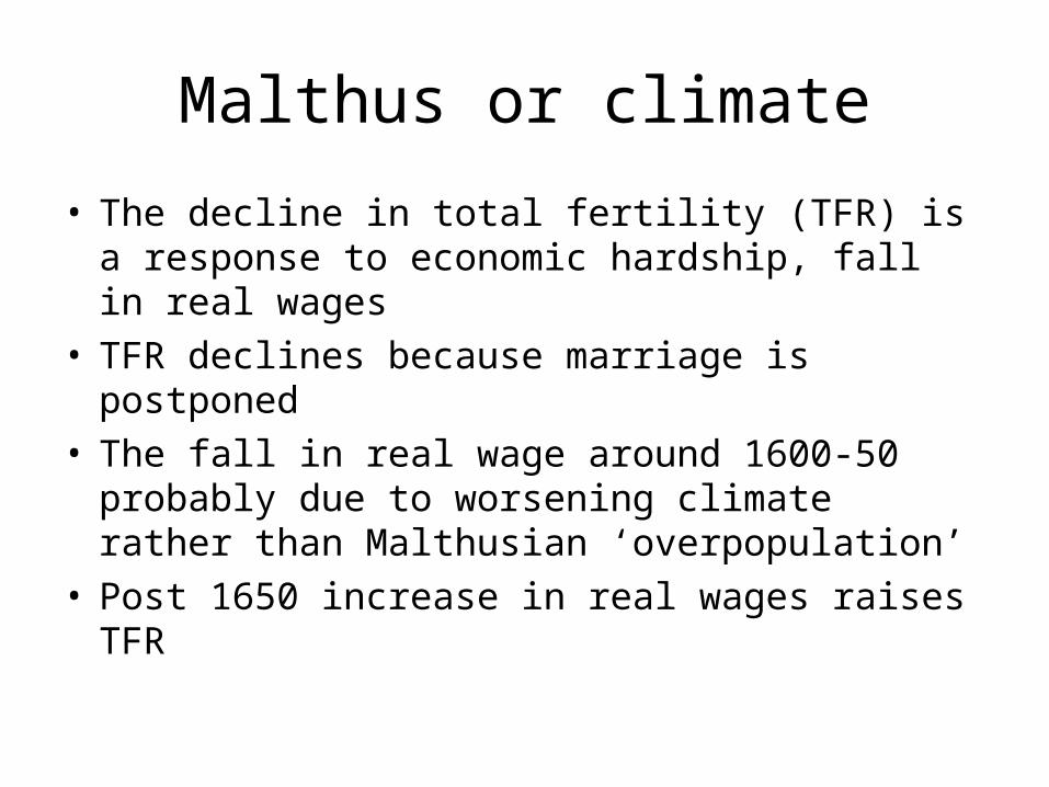
• The decline in total fertility (TFR) is a response to economic hardship, fall in real wages

• TFR declines because marriage is postponed• The fall in real wage around 1600-50 probably

due to worsening climate rather than Malthusian ‘overpopulation’

• Post 1650 increase in real wages raises TFR

-0.9

-0.8

-0.7

-0.6

-0.5

-0.4

-0.3

-0.2

-0.1

0

0

20

40

60

80

100

120

Real farm wages (1860-9=100)

25 per. Mov. Avg. (Temperatur)

Figure 3:3. Real farm wages in England and deviations from Northern hemisphere temperature, 1560-1880

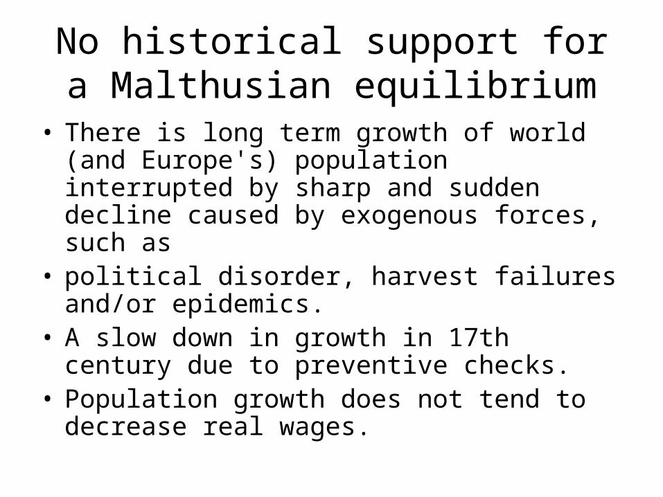
• There is long term growth of world (and Europe's) population interrupted by sharp and sudden decline caused by exogenous forces, such as

• political disorder, harvest failures and/or epidemics.

• A slow down in growth in 17th century due to preventive checks.

• Population growth does not tend to decrease real wages.

No historical support for a Malthusian equilibrium

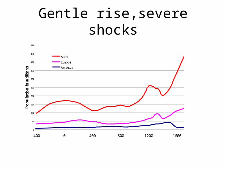
Gentle rise,severe shocks

0

50

100

150

200

250

300

350

400

450

500

-400 0 400 800 1200 1600

Po

pu

lati

on

in

mil

lio

ns

Asia

Europe

America

0

500

1000

1500

2000

2500

3000

3500

4000

1700

1720

1740

1760

1780

1800

1820

1840

1860

1880

1900

1920

1940

1960

1980

2000

Po

pu

lati

on

in

mil

lio

ns

America

Europe

Asia

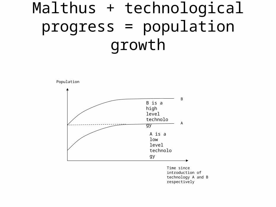
Malthus + technological progress = population growth

Population

Time since introduction of technology A and B respectively

A

B

A is a low level technology

B is a high level technology

The meaning of land constraint

• There are about 13 billion of hectares of landmass

• With current technology about 7 billion hectares are unfit for agriculture

• The land constraint is then 6 billion hectares

• 5 to 5.5 billion hectares are currently used

But, land is a constraint only at a given level of technology

• The most advanced types of agriculture have up to two crops per unit and year, crop ratio = 2.

• Primitive agriculture - slash and burn – has a crop ratio of 0.05

• The difference between the two is a multiple of 40

• Technological progress is ’land-augmenting’

Substitutes for land

• Scarcity of land triggers off other yield increasing inputs such as

• manure from man and animals, seaweed and in exceptional cases: herring (!!!)

• water (irrigation schemes)

• capital, for example better ploughs and stronger draught animals, horses

• high yield crops

Modern poulation dynamics

• cbr fall with increasing income contrary to Malthus prediction

• cdr have arrived at a low steady state level

• Population growth is low again

• Analyze that!

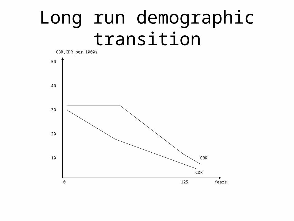
Long run demographic transition

0 125

50

40

30

20

10 CBR

CDR

CBR,CDR per 1000s

Years

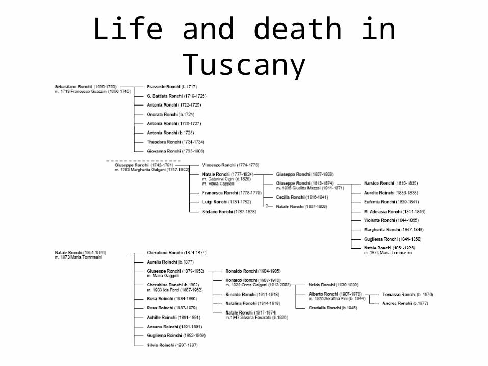
Life and death in Tuscany

From high pressure to low pressure demographic regimes

• Pre-industrial economies have high fertility and high mortality. (High pressure)

• Look at the infant mortality!

• Life expectancy is low.

• The transition to the modern low pressure (low fertility and low mortality) comes late and is fast in this village.

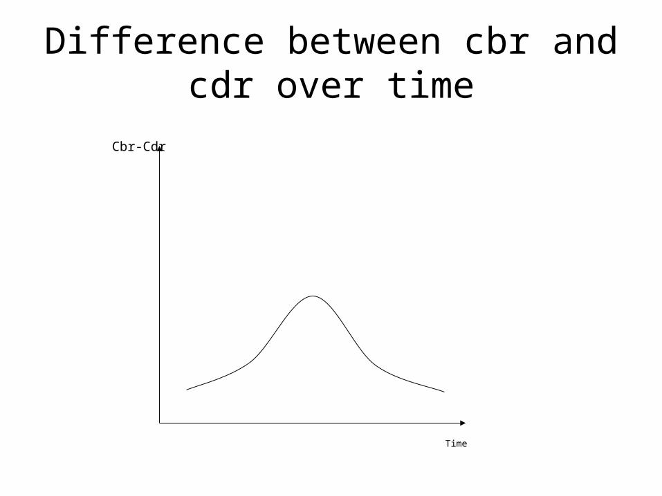
Difference between cbr and cdr over time

Time

Cbr-Cdr

The demographic transition

20 30 40 50 60 70 80

Life expectancy at birth

Childeren per woman(TFR)

17th-18thold regime 0.1- 0.4 percent growth of population

20th Modern regime0.1- 0.4 percent growth of population

0

1

2

5

4

3

6

Transition regime,19th century 1-1.5 percent growth of population

Why fertility falls with increasing income

• Assume that parents get utility (pleasure) from the presence of kids, now and in the future – sometimes hard to believe, but…

• Malthus implicitly believed that utility derived from the number of kids since only income constraints stopped households from having the maximum number

Quality vs. Quantity

• It seems more plausible that the utility is derived from the quality and quantity of kids

• There will be a trade off between quality and quantity of kids and between other goods

• Given the income constraint you cannot have better quality if you do not sacrifice quantity, or the other way around.

Theory becomes ambiguous

• If quality and quantity are a normal goods • then consumption of the both will increase

with increasing income (income effect)• but theory does not tell you about the

income elasticity for quality and quantity being a matter of culture and taste, which can change over time

• Modern households prefer quality over quantity: less but better

Don’t forget the substitution effect!!

• Raising kids is time intensive and if wages increase the opportunity costs of having and educating kids increase.

• The substitution effect, negative on demand for kids, in particular the numbers, might be stronger than the positive income effect.

Why do well educated women have fewer kids?

• The opportunity cost having kids is higher because high education promotes high wages.

• Substitution effect (negative on demand for kids) stronger than postive income effect.

Reflect on this graph! trend growth and growth after a negative population shock. What do

you see?

Summary

• Malthus predicted that population growth would depress real wages and population growth would eventually come to a halt

• However, technological progress seems to keep real wages at a constant or slowly increasing level despite continuing population growth in pre-industrial economies.

• It seems as if population growth can stimulate technological progress and division of labour. More about that next time.