Lecture 3: Applications of Basic Equations

ESS228Prof. Jin-Yi Yu

Lecture 3: Applications of Basic Equations

• Pressure Coordinates: Advantage and Disadvantage • Momentum Equation Balanced Flows • Thermodynamic & Momentum Eq.s Thermal Wind Balance • Continuity Equation Surface Pressure Tendency • Trajectories and Streamlines • Ageostrophic Motion


Pressure as Vertical Coordinate

• From the hydrostatic equation, it is clear that a single valued monotonic relationship exists between pressure and height in each vertical column of the atmosphere.

• Thus we may use pressure as the independent vertical coordinate.

• Horizontal partial derivatives must be evaluated holding p constant.

How to treat the horizontal pressure gradient force?


Horizontal Derivatives on Pressure Coordinate

Using the hydrostatic balance equation

x-component of pressure gradient force =

y-component of pressure gradient force =



Horizontal Momentum Eq. Scaled for Midlatitude Synoptic-Scale

Z-Coordinate

P-Coordinate


Geopotential ( ) and Geopotential Height (Z)The work required to raise a unit mass from the surface of the Earth to some height z is called the geopotential, which is defined as:

The geopotential height is defined as:

The geopotential height is approximately equal to the actual height. However, for dynamic calculations involving the wind the geopotential height must be used for maximum accuracy, since even small deviations can lead to errors in the wind.

ESS124Prof. Jin-Yi YuESS124Prof. Jin-Yi Yu

Pressure Surface• A pressure surface is a surface

above the ground where the pressure has a specific value, such as 700mb.

• Constant pressure surfaces slope downward from the warm to the cold side.

• Since the atmosphere in the polar regions is cold and the tropical atmosphere is warm, all pressure surfaces in the troposphere slope downward from the tropics to the polar regions.

ESS124Prof. Jin-Yi YuESS124Prof. Jin-Yi Yu

Height (Pressure) Map at a Constant Pressure (Height)• Since the atmosphere in the polar

regions is cold and the tropical atmosphere is warm, all pressure surfaces in the troposphere slope downward from the tropics to the polar regions.

• The pressure information on a constant altitude allow us to visualize where high- and low-pressure centers are located.

• The height information on a constant pressure surface convey the same information.

• The intensity of the pressure (or height) gradients allow us to infer the strength of the winds.At 5700m

At 500mb


Advantage of Using P-Coordinate

• Thus in the isobaric coordinate system the horizontal pressure gradient force is measured by the gradient of geopotential at constant pressure.

• Density no longer appears explicitly in the pressure gradient force; this is a distinct advantage of the isobaric system.

• Thus, a given geopotential gradient implies the same geostrophic wind at any height, whereas a given horizontal pressure gradient implies different values of the geostrophic wind depending on the density.


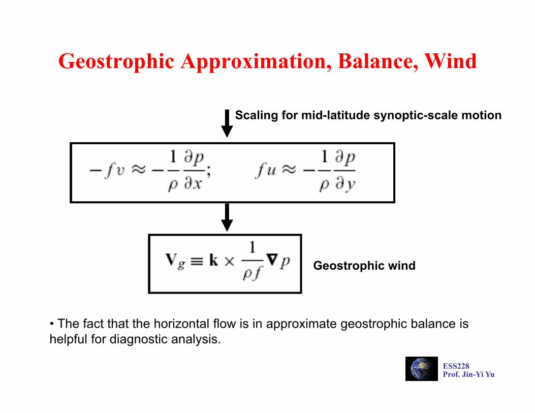
Geostrophic Approximation, Balance, Wind

Scaling for mid-latitude synoptic-scale motion

Geostrophic wind

• The fact that the horizontal flow is in approximate geostrophic balance is helpful for diagnostic analysis.


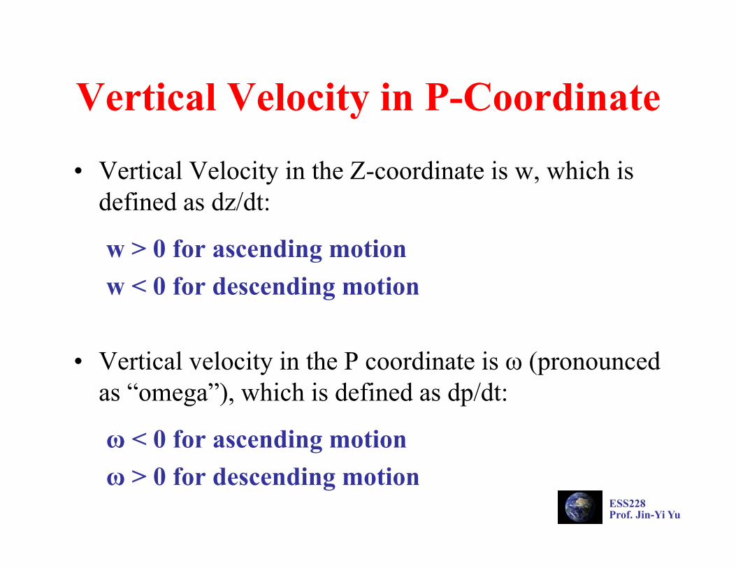
Vertical Velocity in P-Coordinate

• Vertical Velocity in the Z-coordinate is w, which is defined as dz/dt:

w > 0 for ascending motionw < 0 for descending motion

• Vertical velocity in the P coordinate is ω (pronounced as “omega”), which is defined as dp/dt:

ω < 0 for ascending motionω > 0 for descending motion


Continuity Eq. on P-Coordinate

• Following a control volume (δV= δxδyδz = -δxδyδp/ρg using hydrostatic balance), the mass of the volume does not change:

Using

Simpler! No density variations involved in this form of continuity equation.

ρ.δV


Velocity Divergence Form (Lagragian View)

• Following a control volume of a fixed mass (δ M), the amount of mass is conserved.

• and


Thermodynamic Eq. on P-Coordinate

• This form is similar to that on the Z-coordinate, except that there is a strong height dependence of the stability measure (Sp), which is a minor disadvantage of isobaric coordinates.


Scaling of the Thermodynamic Eq.

Small terms; neglected after scaling

Г= -әT/ әz = lapse rateГd= -g/cp = dry lapse rate


Balanced Flows

Cyclostrophic FlowGeostrophic Flow Gradient Flow

Rossby Number

Small ~ 1 Large

Despite the apparent complexity of atmospheric motion systems as depicted onsynoptic weather charts, the pressure (or geopotential height) and velocity distributions in meteorological disturbances are actually related by rather simple approximate force balances.


Scaling Results for the Horizontal Momentum Equations


Rossby Number

• Rossby number is a non-dimensional measure of the magnitude of the acceleration compared to the Coriolis force:

• The smaller the Rossby number, the better the geostrophic balance can be used.


Geostrophic Motion

“Geo” Earth“Strophe” Turning


Natural Coordinate

• At any point on a horizontal surface, we can define a pair of a system of natural coordinates (t, n), where t is the length directed downstream along the local streamline, and n is distance directed normal to the streamline and toward the left.

t

s


Coriolis and Pressure Gradient Force

• Because the Coriolis force always acts normal to the direction of motion, its natural coordinate form is simply in the following form:

• The pressure gradient force can be expressed as:


Acceleration Term in Natural Coordinate

Therefore, the acceleration following the motion is the sum of the rate of change of speed of the air parcel and its centripetal acceleration due to the curvature of the trajectory.


Horizontal Momentum Eq. (on Natural Coordinate)


Geostrophic Balance

Flow in a straight line (R → ± ∞) parallel to height contours is referred to as geostrophic motion. In geostrophic motion the horizontal components of the Coriolis force and pressure gradient force are in exact balance so that V = Vg.


Cyclostrophic Balance

• If the horizontal scale of a disturbance is small enough, the Coriolis force may be neglected compared to the pressure gradient force and the centrifugal force. The force balance normal to the direction of flow becomes in cyclostrophic balance.

• An example of cyclostrophic scale motion is tornado.

• A cyclostrophic motion can be either clockwise or counter-clockwise.

Only low pressure system can have cyclostrophic flow.


Gradient Balance

• Horizontal frictionless flow that is parallel to the height contours so that the tangential acceleration vanishes (DV/Dt = 0) is called gradient flow.

• Gradient flow is a three-way balance among the Coriolis force, the centrifugal force, and the horizontal pressure gradient force.

• The gradient wind is often a better approximation to the actual wind than the geostrophic wind.


Super- and Sub-Geostrophic Wind

(from Meteorology: Understanding the Atmosphere)

For high pressure system

gradient wind > geostrophic wind

supergeostropic.

For low pressure system

gradient wind < geostrophic wind

subgeostropic.


Upper Tropospheric Flow Pattern

• Upper tropospheric flows are characterized by trough (low pressure; isobars dip southward) and ridge (high pressure; isobars bulge northward).

• The winds are in gradient wind balance at the bases of the trough and ridge and are slower and faster, respectively, than the geostrophic winds.

• Therefore, convergence and divergence are created at different parts of the flow patterns, which contribute to the development of the low and high systems.


Convergence/Divergence and Vertical Motion

• Convergence in the upper tropospheric flow pattern can cause descending motion in the air column. surface pressure increase (high pressure) clear sky

• Divergence in the upper troposphric flow pattern ca cause ascending motion in the air column. surface pressure decreases (low pressure) cloudy weather



Convergence/Divergence in Jetstreak


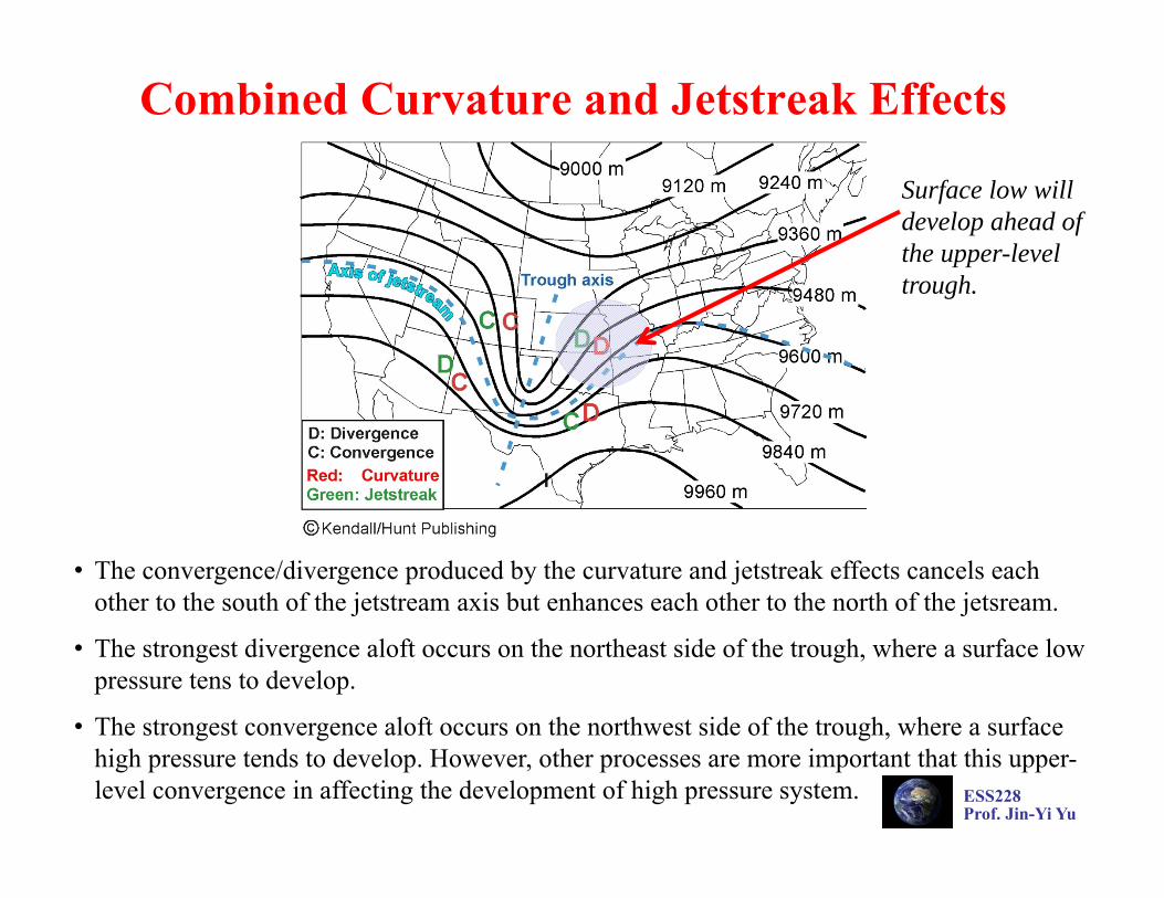
Combined Curvature and Jetstreak Effects

• The convergence/divergence produced by the curvature and jetstreak effects cancels each other to the south of the jetstream axis but enhances each other to the north of the jetsream.

• The strongest divergence aloft occurs on the northeast side of the trough, where a surface low pressure tens to develop.

• The strongest convergence aloft occurs on the northwest side of the trough, where a surface high pressure tends to develop. However, other processes are more important that this upper-level convergence in affecting the development of high pressure system.

Surface low will develop ahead of the upper-level trough.


Developments of Low- and High-Pressure Centers• Dynamic Effects: Combined curvature

and jetstreak effects produce upper-level convergence on the west side of the trough to the north of the jetsreak, which add air mass into the vertical air column and tend to produce a surface high-pressure center. The same combined effects produce a upper-level divergence on the east side of the trough and favors the formation of a low-level low-pressure center.

• Frictional Effect: Surface friction will cause convergence into the surface low-pressure center after it is produced by upper-level dynamic effects, which adds air mass into the low center to “fill” and weaken the low center (increase the pressure)

• Low Pressure: The evolution of a low center depends on the relative strengths of the upper-level development and low-level friction damping.

• High Pressure: The development of a high center is controlled more by the convergence of surface cooling than by the upper-level dynamic effects. Surface friction again tends to destroy the surface high center.

• Thermodynamic Effect: heating surface low pressure; cooling surface high pressure.


Trajectory and Streamline• It is important to distinguish clearly between

streamlines, which give a “snapshot” of the velocity field at any instant, and trajectories, which trace the motion of individual fluid parcels over a finite time interval.

• The geopotential height contour on synoptic weather maps are streamlines not trajectories.

• In the gradient balance, the curvature (R) is supposed to be the estimated from the trajectory, but we estimate from the streamlines from the weather maps.


Thermal Wind Balance(1) Geostrophic Balance

(2) Hydrostratic Balance

Combine (1) and (2)


Physical Meanings

• The thermal wind is a vertical shear in the geostrophic wind caused by a horizontal temperature gradient. Its name is a misnomer, because the thermal wind is not actually a wind, but rather a wind gradient.

• The vertical shear (including direction and speed) of geostrophic wind is related to the horizontal variation of temperature.

The thermal wind equation is an extremely useful diagnostic tool, which is often used to check analyses of the observed wind and temperature fields for consistency.

It can also be used to estimate the mean horizontal temperature advection in a layer. Thermal wind blows parallel to the isotherms with the warm air to the right facing

downstream in the Northern Hemisphere.


Backing and Veering Winds

Backing Winds

V1

V2

V3

Cold Advection

Wind vectors rotate counter-clockwise with height

Veering Winds

V3

V2

V1

Warm Advection

Wind vectors rotate clockwise with height


Hodographs

• Meteorologists use hodographs to display the vertical wind shear information collected from rawinsondes.

• The change of wind direction and speed between two altitudes is called vertical wind shear.

• Hodographs show wind speed and direction at evenly spaced altitudes, for example at 0.5, 1.0, 1.5, and 2.0 kilometers.


Information on a Hodograph• Wind Speed: distance from the

center of the hodograph denotes wind speed.

• Wind Direction: each dot on the hodograph can be regarded as the head of an arrow pointing from the diagram center in the direction the air is moving.

• Vertical Wind Shear: The length of a line between two points denotes wind speed shear.

• This is a hodograph of a severe thunderstorm that usually forms in an environment with a strong wind shear.


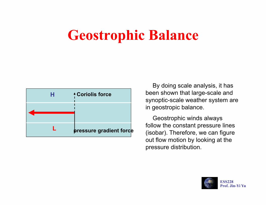
Geostrophic Balance

L

H

pressure gradient force

Coriolis force By doing scale analysis, it has been shown that large-scale and synoptic-scale weather system are in geostropic balance.

Geostrophic winds always follow the constant pressure lines (isobar). Therefore, we can figure out flow motion by looking at the pressure distribution.


Vertical Motions

• For synoptic-scale motions, the vertical velocity component is typically of the order of a few centimeters per second. Routine meteorological soundings, however, only give the wind speed to an accuracy of about a meter per second.

• Thus, in general the vertical velocity is not measured directly but must be inferred from the fields that are measured directly.

• Two commonly used methods for inferring the vertical motion field are (1) the kinematic method, based on the equation of continuity, and (2) the adiabatic method, based on the thermodynamic energy equation.


The Kinematic Method• We can integrate the continuity equation in the vertical to get the vertical

velocity.

• We use the information of horizontal divergence to infer the vertical velocity. However, for midlatitude weather, the horizontal divergence is due primarily to the small departures of the wind from geostrophic balance. A 10% error in evaluating one of the wind components can easily cause the estimated divergence to be in error by 100%.

• For this reason, the continuity equation method is not recommended for estimating the vertical motion field from observed horizontal winds.


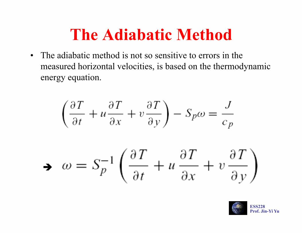
The Adiabatic Method• The adiabatic method is not so sensitive to errors in the

measured horizontal velocities, is based on the thermodynamic energy equation.


Barotropic and Baroclinic AtmosphereBarotropic Atmosphereno temperature gradient on pressure surfaces isobaric surfaces are also the isothermal surfaces density is only function of pressure ρ=ρ(p) no thermal wind no vertical shear for geostrophic winds geostrophic winds are independent of height you can use a one-layer model to represent the

barotropic atmosphere


Barotropic and Baroclinic AtmosphereBaroclinic Atmospheretemperature gradient exists on pressure surfaces density is function of both pressure and temperature ρ=ρ(p, T)

thermal wind existsgeostrophic winds change with height you need a multiple-layer model to represent the

baroclinic atmosphere

Lecture 3: Applications of Basic Equations

Documents