Lecture 21: Multiple-view geometry and structure from motion CS6670: Computer Vision Noah Snavely.

Lecture 21: Multiple-view geometry and structure from motion

CS6670: Computer VisionNoah Snavely

Readings

• Szeliski, Chapter 7.1 – 7.4

Announcements

• Project 2b due next Tuesday, Nov 2, by 10:59pm

• Final project proposals due by this Friday, Oct 29, by 11:59pm– See project webpage for project ideas

Two-view geometry

• Where do epipolar lines come from?

epipolar plane

epipolar lineepipolar lineepipolar lineepipolar line

0

3d point lies somewhere along r

(projection of r)

Image 1 Image 2

Fundamental matrix

• This epipolar geometry of two views is described by a Very Special 3x3 matrix , called the fundamental matrix

• maps (homogeneous) points in image 1 to lines in image 2!• The epipolar line (in image 2) of point p is:

• Epipolar constraint on corresponding points:

epipolar plane

epipolar lineepipolar lineepipolar lineepipolar line

0

(projection of ray)

Image 1 Image 2

Fundamental matrix

• Two special points: e1 and e2 (the epipoles): projection of one camera into the other

epipolar plane

epipolar lineepipolar lineepipolar lineepipolar line

0

(projection of ray)

Relationship with homography?

Images taken from the same center of projection? Use a homography, and map points directly to points!

Images taken from different places? We need an F-matrix.

Fundamental matrix – uncalibrated case

0

the Fundamental matrix

: intrinsics of camera 1 : intrinsics of camera 2

: rotation of image 2 w.r.t. camera 1

Cross-product as linear operator

Useful fact: Cross product with a vector t can be represented as multiplication with a (skew-symmetric) 3x3 matrix

Fundamental matrix – calibrated case

0

: ray through p in camera 1’s (and world) coordinate system

: ray through q in camera 2’s coordinate system

{the Essential matrix

Properties of the Fundamental Matrix

• is the epipolar line associated with

• is the epipolar line associated with

• and

• is rank 2

• How many parameters does F have?11

T

Rectified case

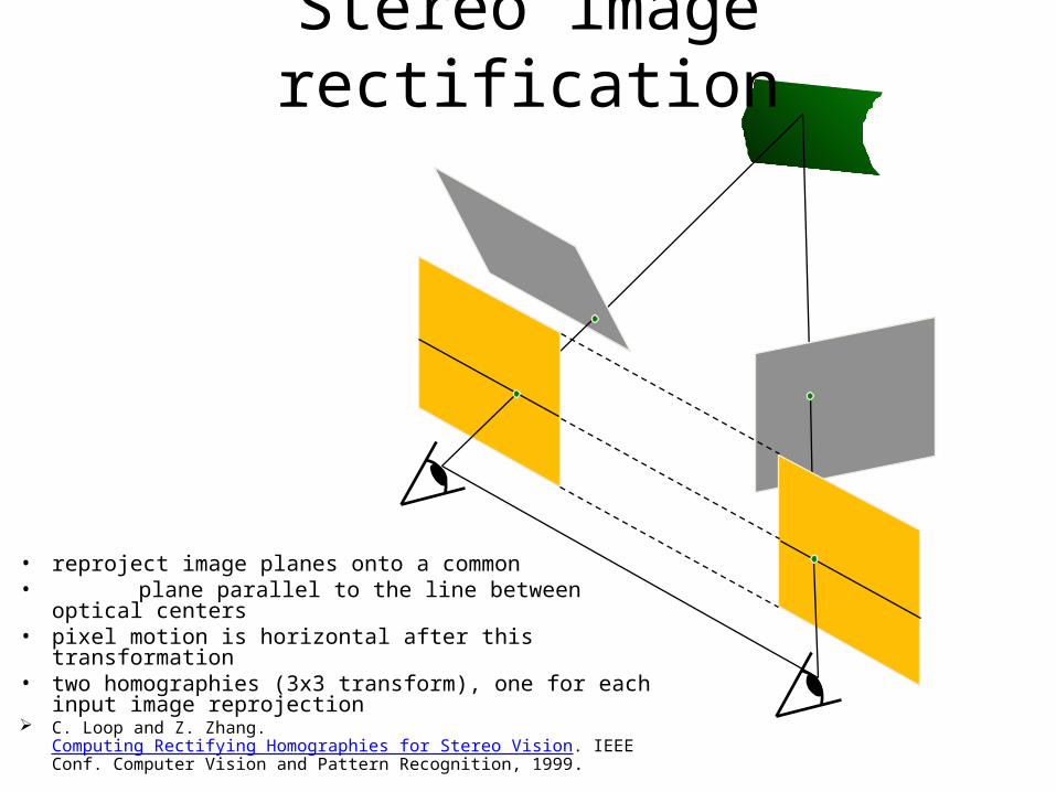
Stereo image rectification

• reproject image planes onto a common• plane parallel to the line between optical centers• pixel motion is horizontal after this transformation• two homographies (3x3 transform), one for each input

image reprojection C. Loop and Z. Zhang. Computing Rectifying Homographies for Stereo Vision.

IEEE Conf. Computer Vision and Pattern Recognition, 1999.

Questions?

Estimating F

• If we don’t know K1, K2, R, or t, can we estimate F for two images?

• Yes, given enough correspondences

Estimating F – 8-point algorithm

• The fundamental matrix F is defined by

0Fxx'

for any pair of matches x and x’ in two images.

• Let x=(u,v,1)T and x’=(u’,v’,1)T,

333231

232221

131211

fff

fff

fff

F

each match gives a linear equation

0'''''' 333231232221131211 fvfuffvfvvfuvfufvufuu

8-point algorithm

0

1´´´´´´

1´´´´´´

1´´´´´´

33

32

31

23

22

21

13

12

11

222222222222

111111111111

f

f

f

f

f

f

f

f

f

vuvvvvuuuvuu

vuvvvvuuuvuu

vuvvvvuuuvuu

nnnnnnnnnnnn

• In reality, instead of solving , we seek f to minimize , least eigenvector of .

0Af

Af AA

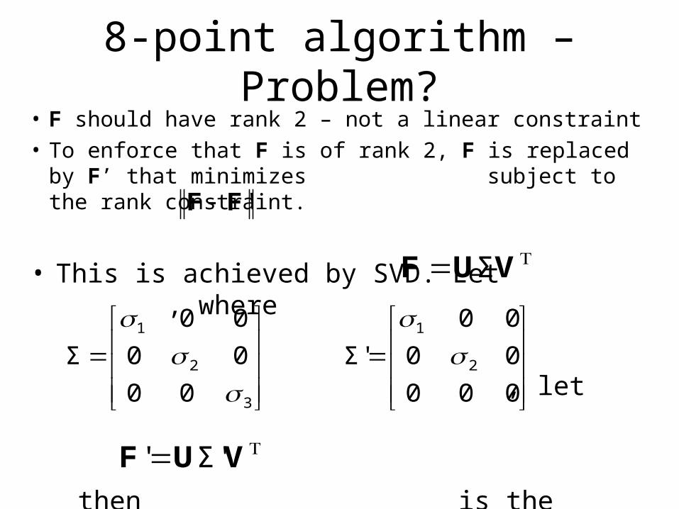
8-point algorithm – Problem?• F should have rank 2 – not a linear constraint• To enforce that F is of rank 2, F is replaced by F’ that

minimizes subject to the rank constraint. 'FF

• This is achieved by SVD. Let , where

, let

then is the solution.

VUF Σ

3

2

1

00

00

00

Σ

000

00

00

Σ' 2

1

VUF Σ''

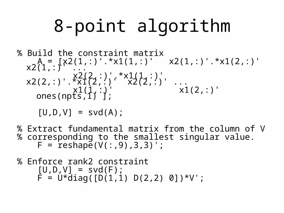
8-point algorithm% Build the constraint matrix A = [x2(1,:)‘.*x1(1,:)' x2(1,:)'.*x1(2,:)' x2(1,:)' ... x2(2,:)'.*x1(1,:)' x2(2,:)'.*x1(2,:)' x2(2,:)' ... x1(1,:)' x1(2,:)' ones(npts,1) ]; [U,D,V] = svd(A); % Extract fundamental matrix from the column of V % corresponding to the smallest singular value. F = reshape(V(:,9),3,3)'; % Enforce rank2 constraint [U,D,V] = svd(F); F = U*diag([D(1,1) D(2,2) 0])*V';

8-point algorithm

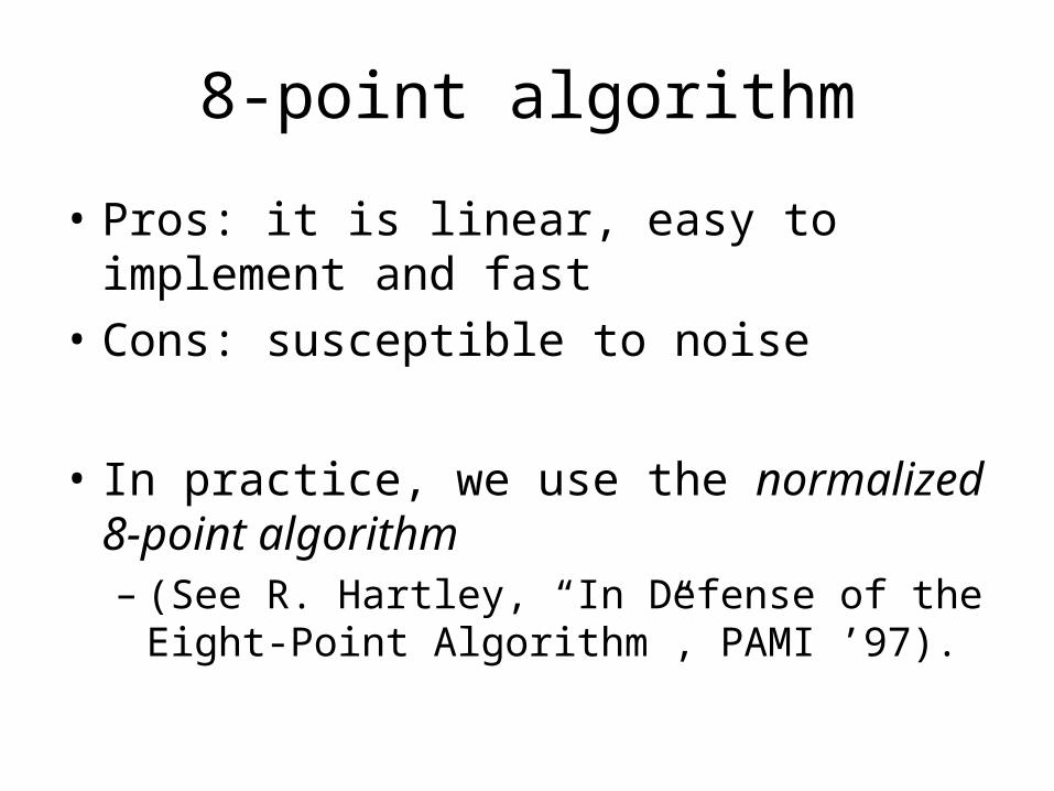
• Pros: it is linear, easy to implement and fast• Cons: susceptible to noise

• In practice, we use the normalized 8-point algorithm– (See R. Hartley, “In Defense of the Eight-Point

Algorithm”, PAMI ’97).

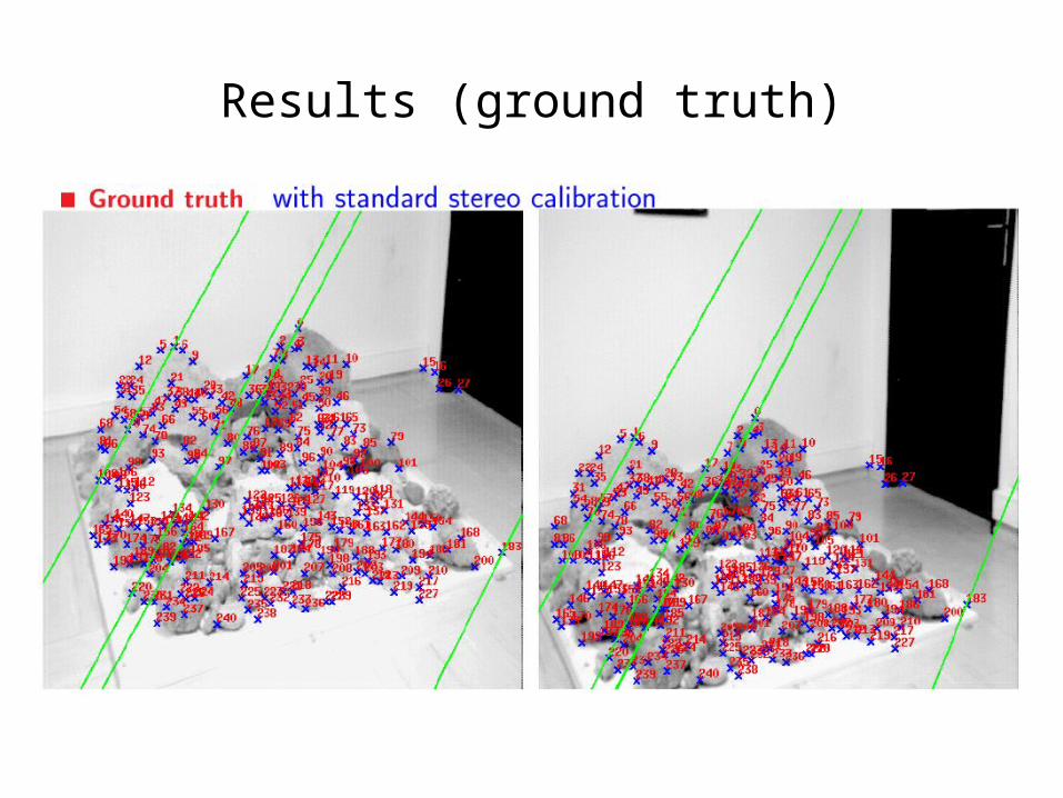
Results (ground truth)

Results (8-point algorithm)

Results (normalized 8-point algorithm)

Estimating the F-matrix

• If we have more than eight points, we can solve a least-squares version of this problem

• What could go wrong?

• How can we fix this?

Estimating the F-matrix

• Extra bonus:– If we run RANSAC to find an F-matrix with the

most inliers, we can throw out inconsistent matches (i.e., this is a “bad match filter”)

– Might be useful later on…

What about more than two views?

• The geometry of three views is described by a 3 x 3 x 3 tensor called the trifocal tensor

• The geometry of four views is described by a 3 x 3 x 3 x 3 tensor called the quadrifocal tensor

• After this it starts to get complicated…