Lecture 20 Object recognition 1

Welcome message from author
This document is posted to help you gain knowledge. Please leave a comment to let me know what you think about it! Share it to your friends and learn new things together.
Transcript

Lecture 20 Object recognition 1
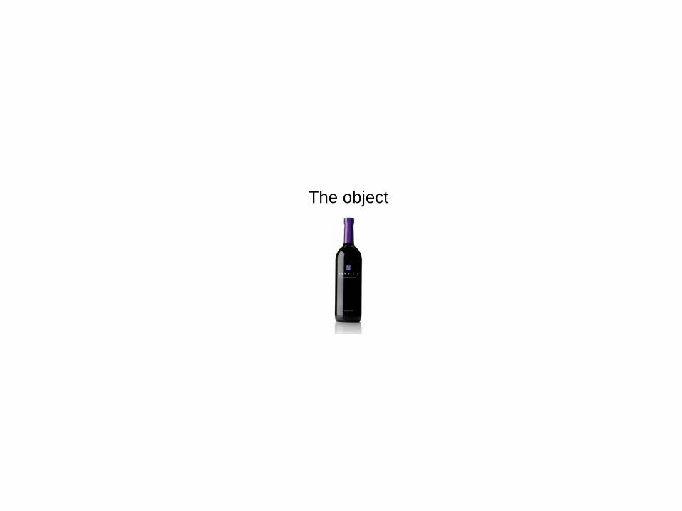
The object
The object
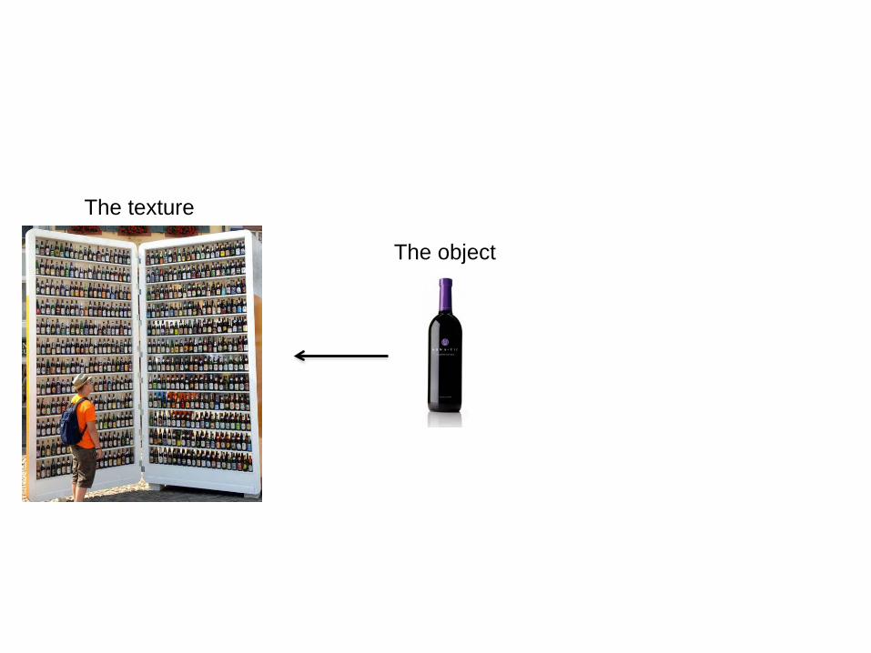
The texture

The object
The texture The scene
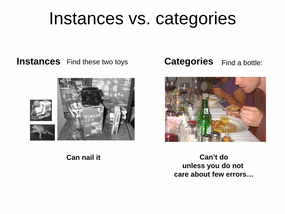
Find a bottle: Categories
Can’t do unless you do not
care about few errors…
Instances Find these two toys
Can nail it
Instances vs. categories

Why do we care about recognition? Perception of function: We can perceive the 3D
shape, texture, material properties, without knowing about objects. But, the concept of category encapsulates also information about what can we do with those objects.
“We therefore include the perception of function as a proper –indeed, crucial- subject for vision science”, from Vision Science, chapter 9, Palmer.
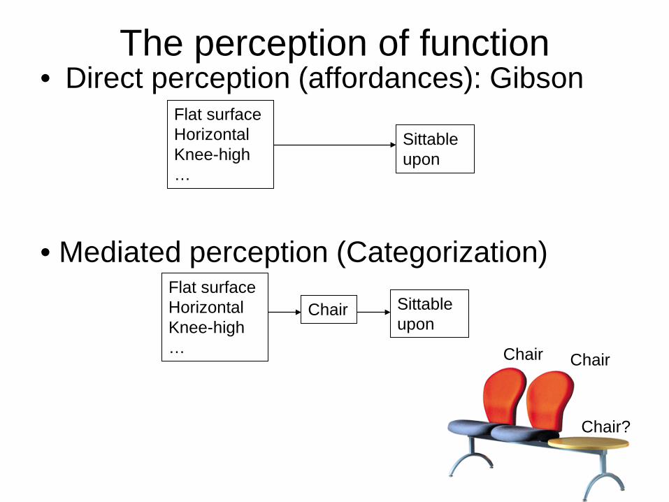
The perception of function • Direct perception (affordances): Gibson
Flat surface Horizontal Knee-high …
Sittable upon
Chair Chair
Chair?
Flat surface Horizontal Knee-high …
Sittable upon
Chair
• Mediated perception (Categorization)
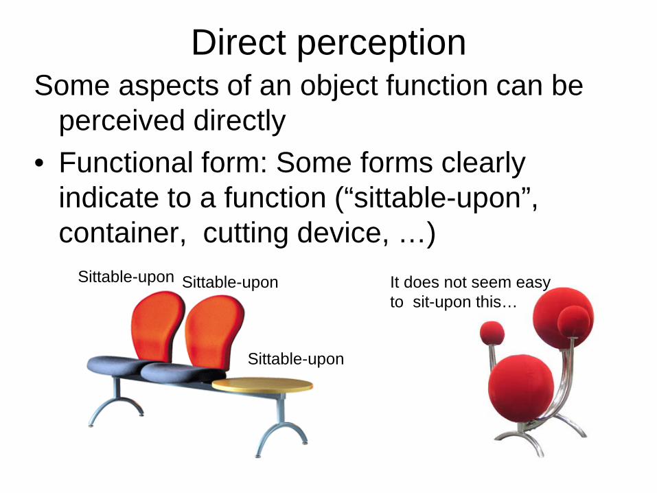
Direct perception Some aspects of an object function can be
perceived directly • Functional form: Some forms clearly
indicate to a function (“sittable-upon”, container, cutting device, …)
Sittable-upon Sittable-upon
Sittable-upon
It does not seem easy to sit-upon this…
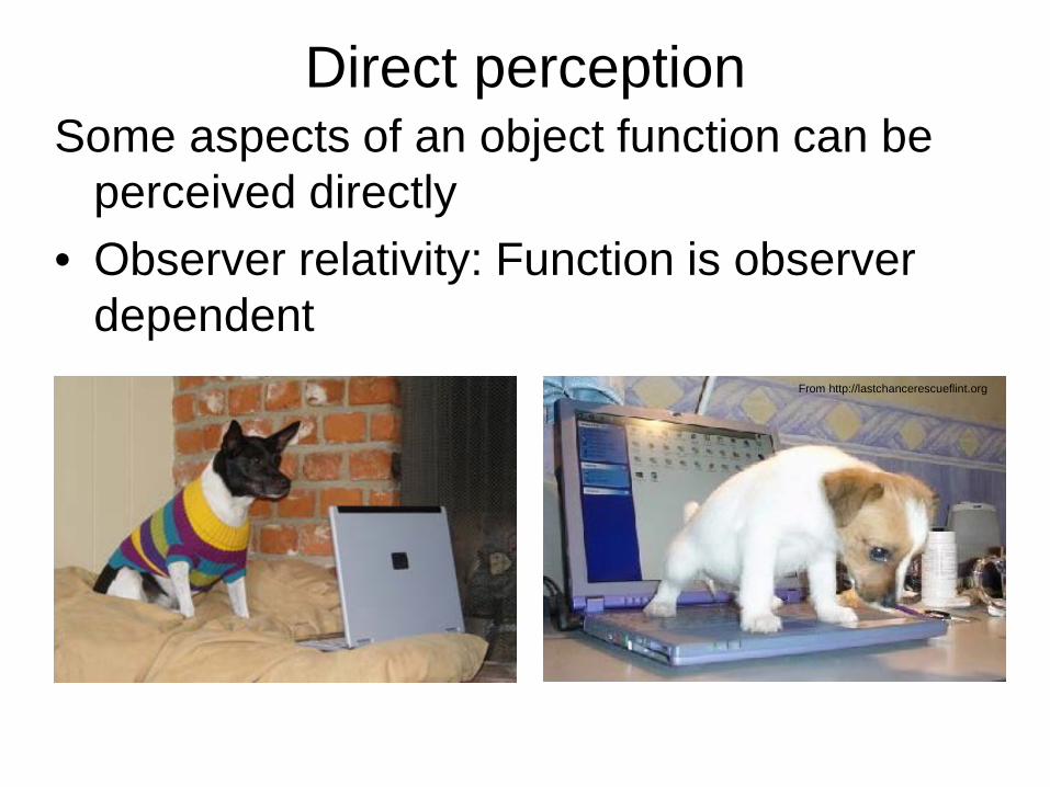
Direct perception Some aspects of an object function can be
perceived directly • Observer relativity: Function is observer
dependent From http://lastchancerescueflint.org

Limitations of Direct Perception
The functions are the same at some level of description: we can put things inside in both and somebody will come later to empty them. However, we are not expected to put inside the same kinds of things…
Objects of similar structure might have very different functions
Not all functions seem to be available from direct visual information only.
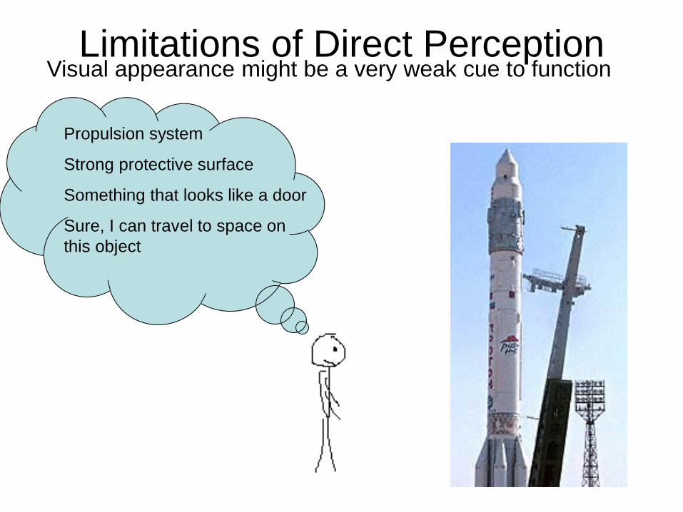
Limitations of Direct Perception
Propulsion system
Strong protective surface
Something that looks like a door
Sure, I can travel to space on this object
Visual appearance might be a very weak cue to function
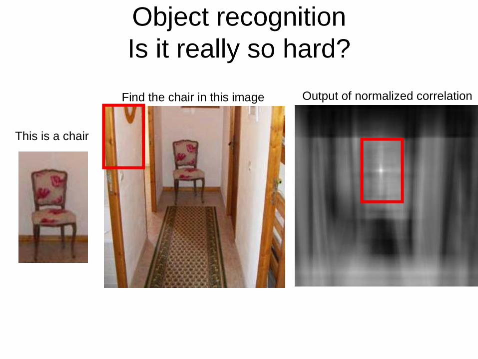
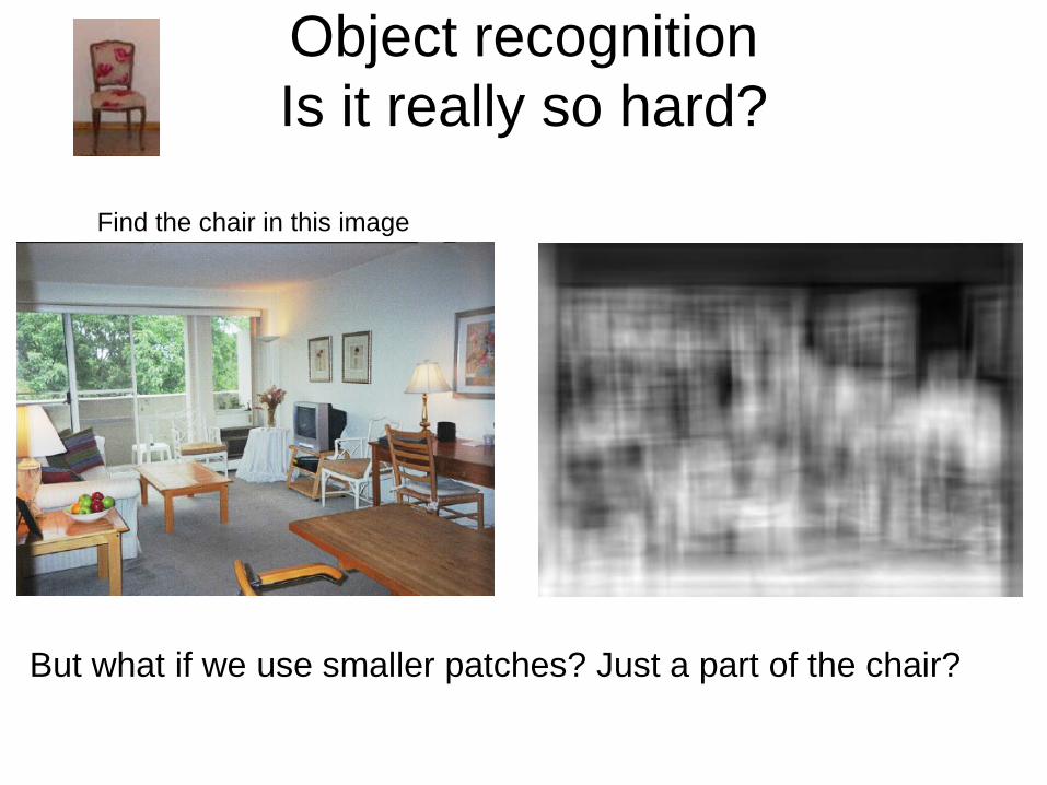
Object recognition Is it really so hard?
This is a chair
Find the chair in this image Output of normalized correlation
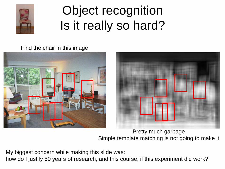
Object recognition Is it really so hard?
My biggest concern while making this slide was: how do I justify 50 years of research, and this course, if this experiment did work?
Find the chair in this image
Pretty much garbage Simple template matching is not going to make it
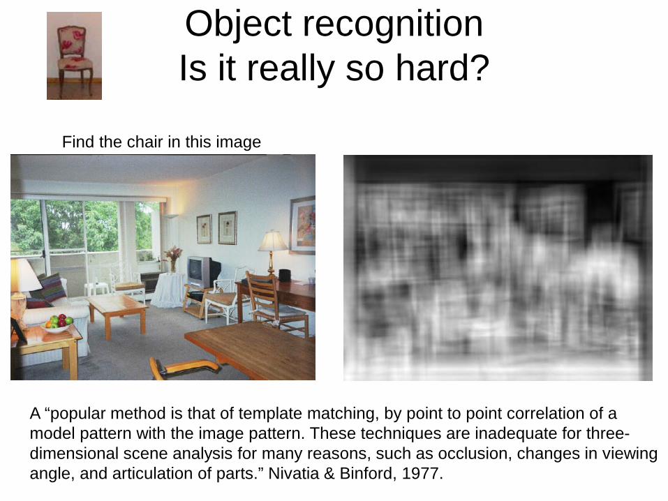
Object recognition Is it really so hard?
Find the chair in this image
A “popular method is that of template matching, by point to point correlation of a model pattern with the image pattern. These techniques are inadequate for three-dimensional scene analysis for many reasons, such as occlusion, changes in viewing angle, and articulation of parts.” Nivatia & Binford, 1977.
Why is object recognition a hard task?
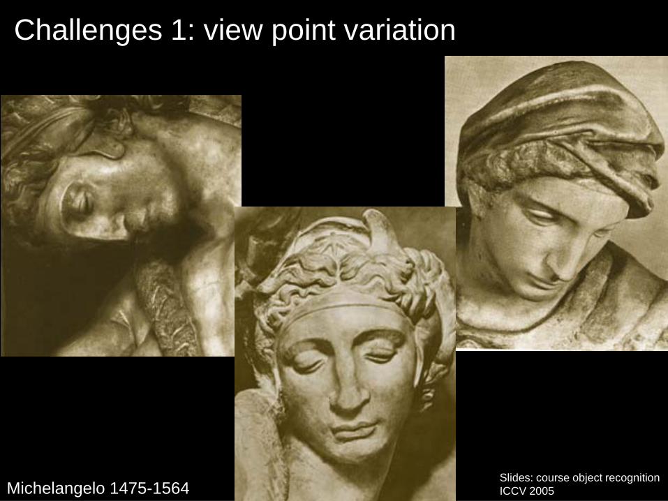
Challenges 1: view point variation
Michelangelo 1475-1564 Slides: course object recognition ICCV 2005
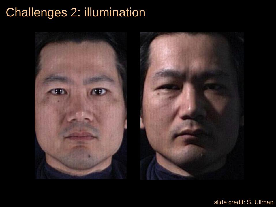
Challenges 2: illumination
slide credit: S. Ullman

Challenges 3: occlusion
Magritte, 1957 Slides: course object recognition ICCV 2005
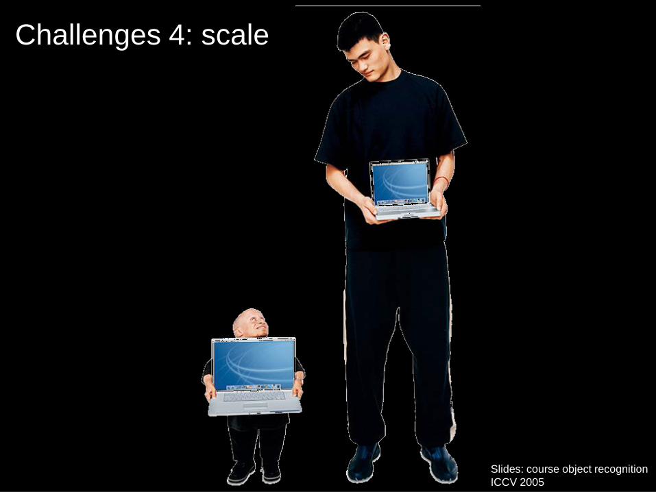
Challenges 4: scale
Slides: course object recognition ICCV 2005
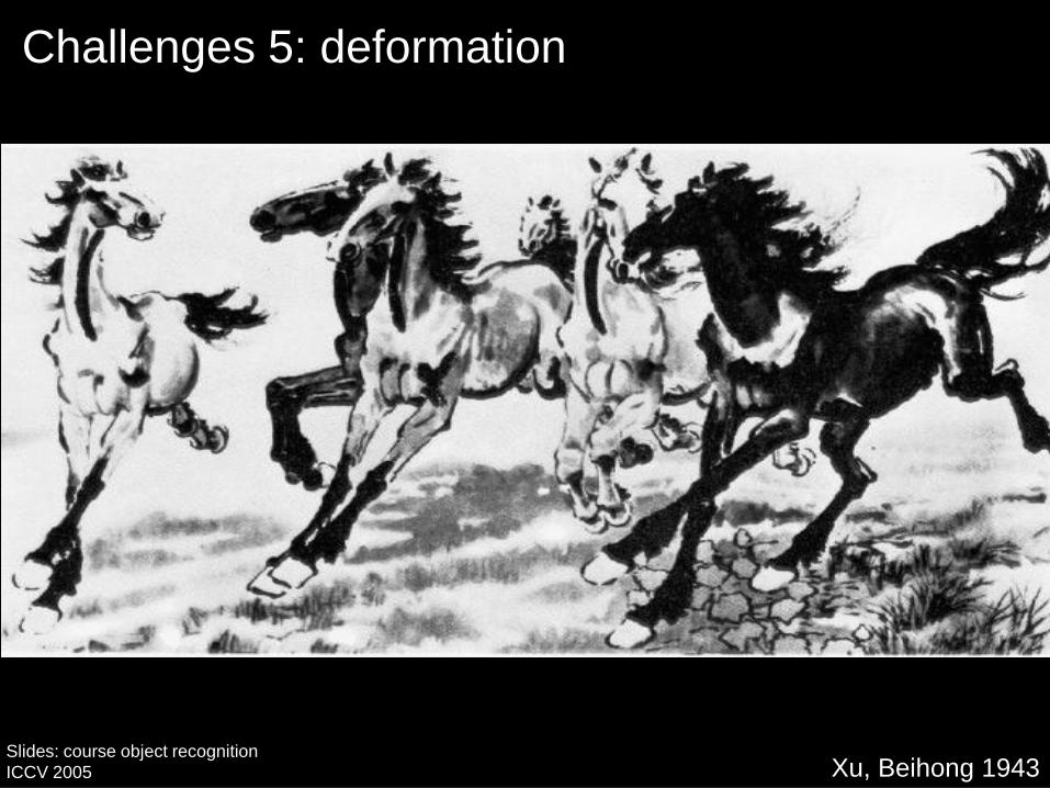
Challenges 5: deformation
Xu, Beihong 1943 Slides: course object recognition ICCV 2005
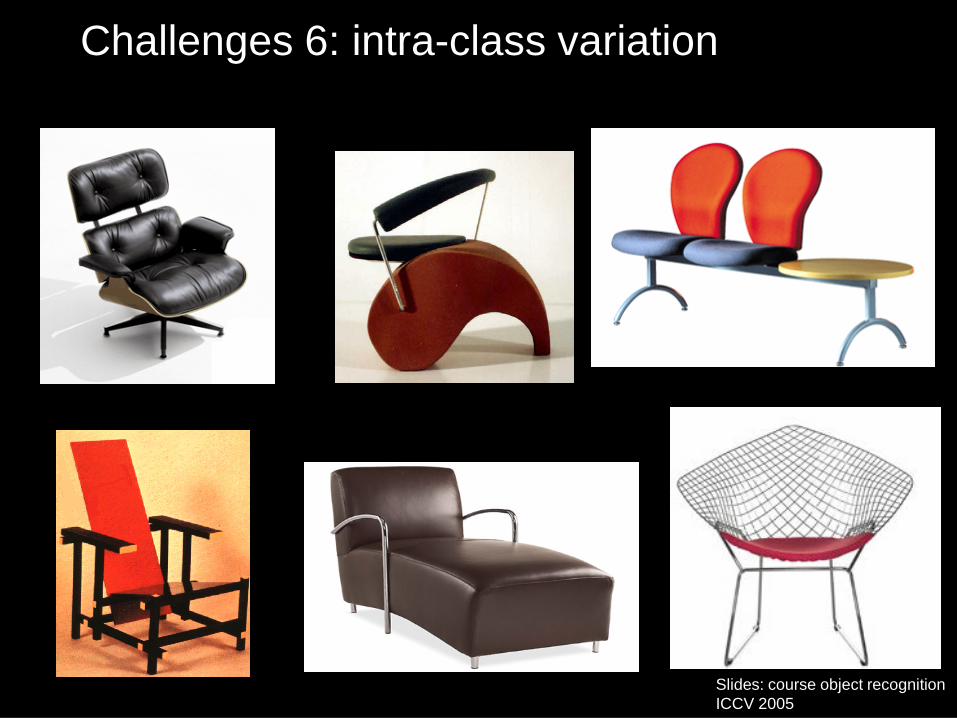
Challenges 6: intra-class variation
Slides: course object recognition ICCV 2005
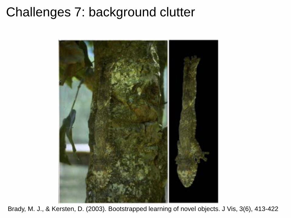
Brady, M. J., & Kersten, D. (2003). Bootstrapped learning of novel objects. J Vis, 3(6), 413-422
Challenges 7: background clutter
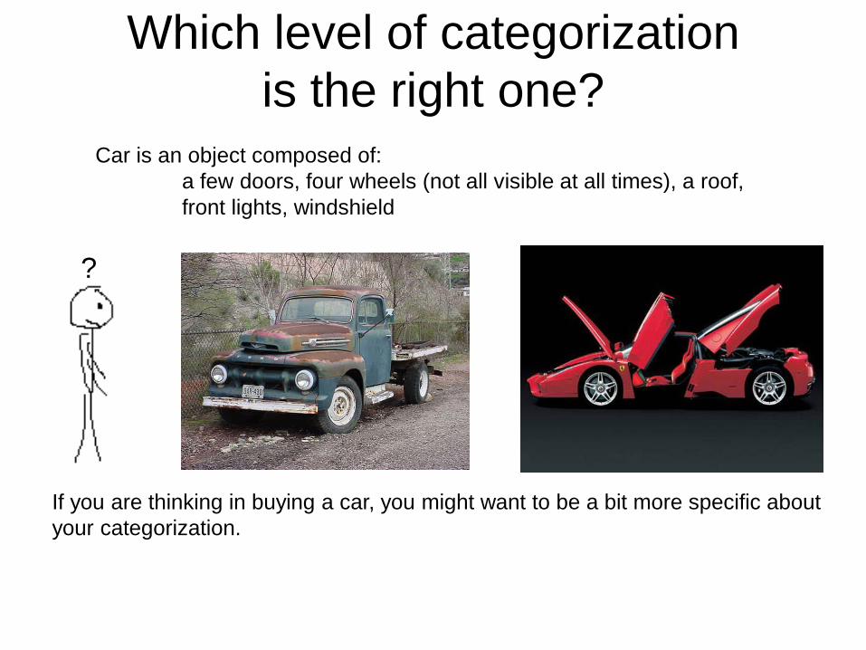
Which level of categorization is the right one?
Car is an object composed of: a few doors, four wheels (not all visible at all times), a roof, front lights, windshield
If you are thinking in buying a car, you might want to be a bit more specific about your categorization.
?
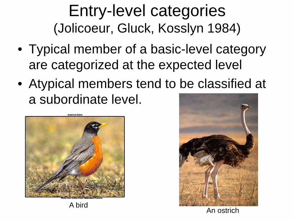
Entry-level categories (Jolicoeur, Gluck, Kosslyn 1984)
• Typical member of a basic-level category are categorized at the expected level
• Atypical members tend to be classified at a subordinate level.
A bird An ostrich

Creation of new categories
A new class can borrow information from similar categories

Yes, object recognition is hard… (or at least it seems so for now…)
Object recognition Is it really so hard?
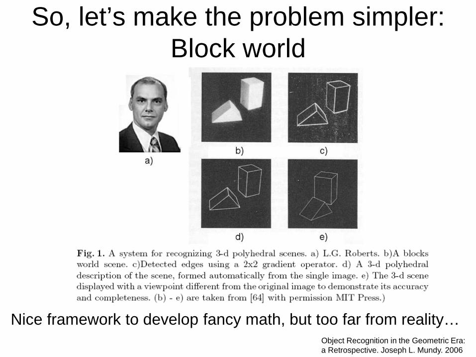
So, let’s make the problem simpler: Block world
Nice framework to develop fancy math, but too far from reality… Object Recognition in the Geometric Era: a Retrospective. Joseph L. Mundy. 2006
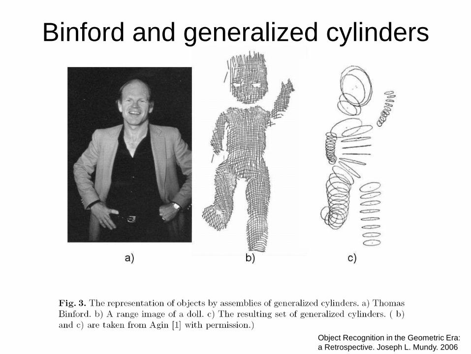
Object Recognition in the Geometric Era: a Retrospective. Joseph L. Mundy. 2006
Binford and generalized cylinders

Binford and generalized cylinders
Recognition by components
Irving Biederman Recognition-by-Components: A Theory of Human Image Understanding. Psychological Review, 1987.

Recognition by components The fundamental assumption of the proposed theory,
recognition-by-components (RBC), is that a modest set of generalized-cone components, called geons (N = 36), can be derived from contrasts of five readily detectable properties of edges in a two-dimensional image: curvature, collinearity, symmetry, parallelism, and cotermination.
The “contribution lies in its proposal for a particular
vocabulary of components derived from perceptual mechanisms and its account of how an arrangement of these components can access a representation of an object in memory.”
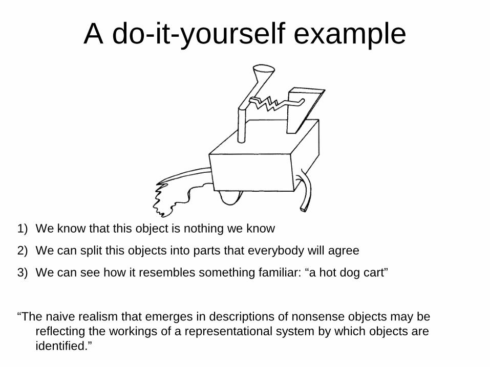
1) We know that this object is nothing we know
2) We can split this objects into parts that everybody will agree
3) We can see how it resembles something familiar: “a hot dog cart”
“The naive realism that emerges in descriptions of nonsense objects may be reflecting the workings of a representational system by which objects are identified.”
A do-it-yourself example

Hypothesis • Hypothesis: there is a small number of geometric
components that constitute the primitive elements of the object recognition system (like letters to form words).
• “The particular properties of edges that are postulated to be relevant to the generation of the volumetric primitives have the desirable properties that they are invariant over changes in orientation and can be determined from just a few points on each edge.”
• Limitation: “The modeling has been limited to concrete entities with specified boundaries.” (count nouns) – this limitation is shared by many modern object detection algorithms.
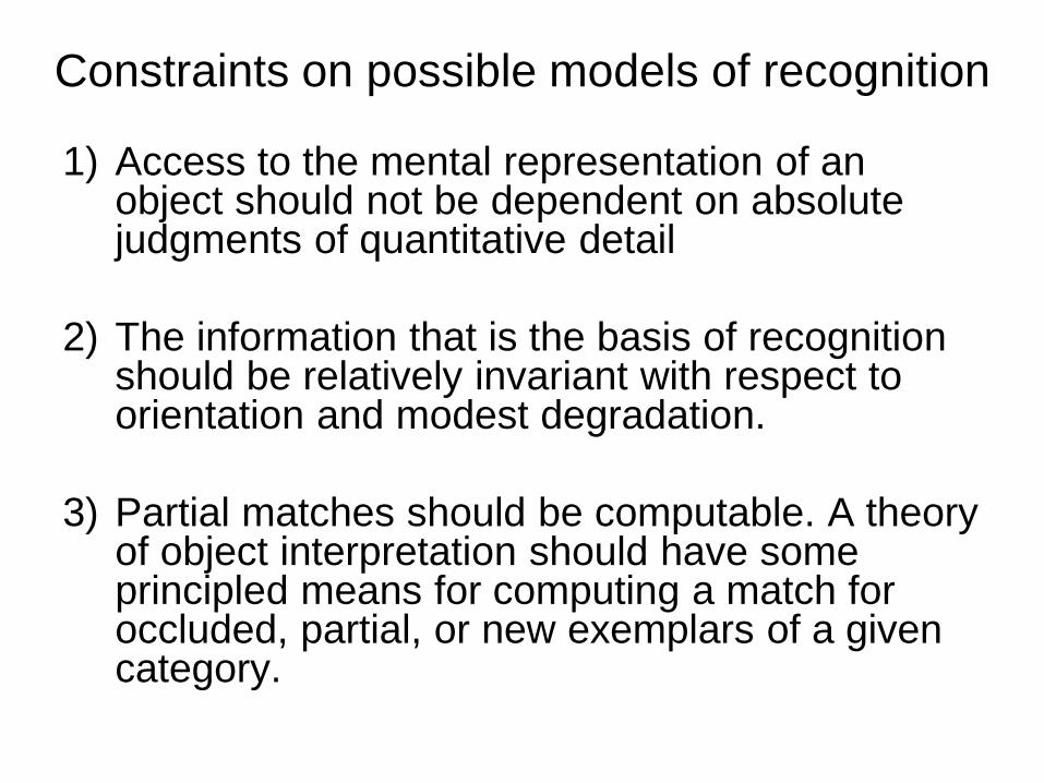
Constraints on possible models of recognition
1) Access to the mental representation of an object should not be dependent on absolute judgments of quantitative detail
2) The information that is the basis of recognition should be relatively invariant with respect to orientation and modest degradation.
3) Partial matches should be computable. A theory of object interpretation should have some principled means for computing a match for occluded, partial, or new exemplars of a given category.
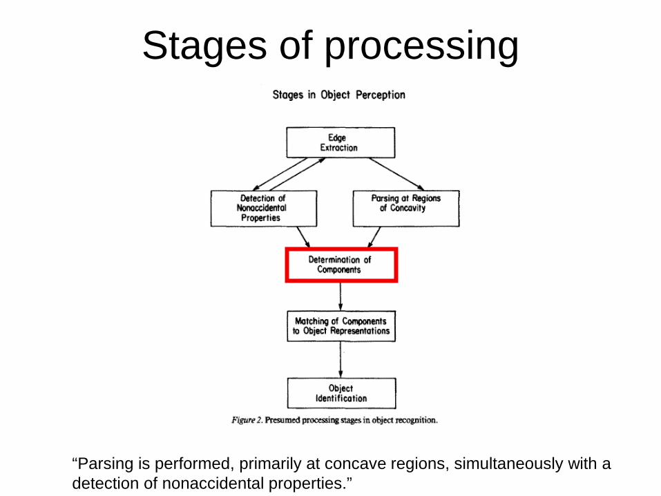
Stages of processing
“Parsing is performed, primarily at concave regions, simultaneously with a detection of nonaccidental properties.”
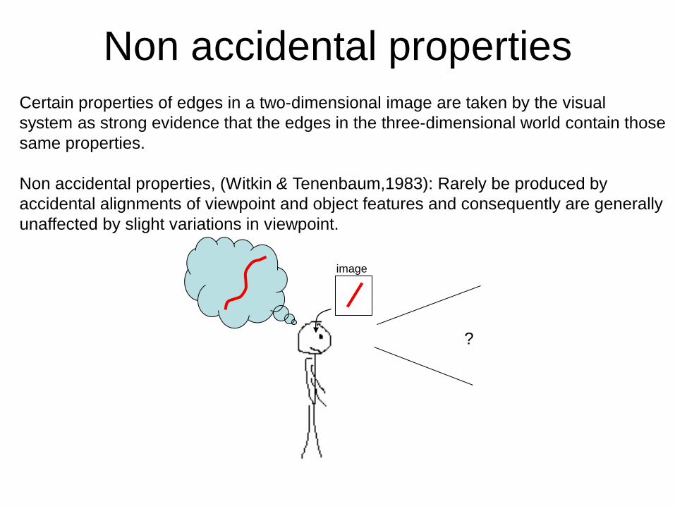
Non accidental properties Certain properties of edges in a two-dimensional image are taken by the visual system as strong evidence that the edges in the three-dimensional world contain those same properties. Non accidental properties, (Witkin & Tenenbaum,1983): Rarely be produced by accidental alignments of viewpoint and object features and consequently are generally unaffected by slight variations in viewpoint.
?
image
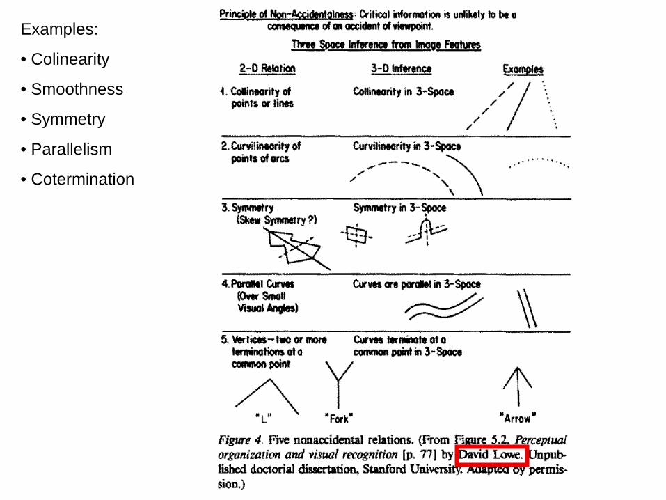
Examples:
• Colinearity
• Smoothness
• Symmetry
• Parallelism
• Cotermination
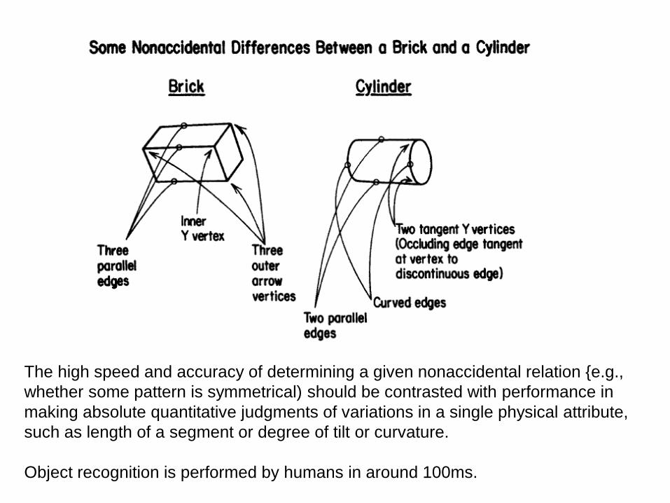
The high speed and accuracy of determining a given nonaccidental relation {e.g., whether some pattern is symmetrical) should be contrasted with performance in making absolute quantitative judgments of variations in a single physical attribute, such as length of a segment or degree of tilt or curvature. Object recognition is performed by humans in around 100ms.
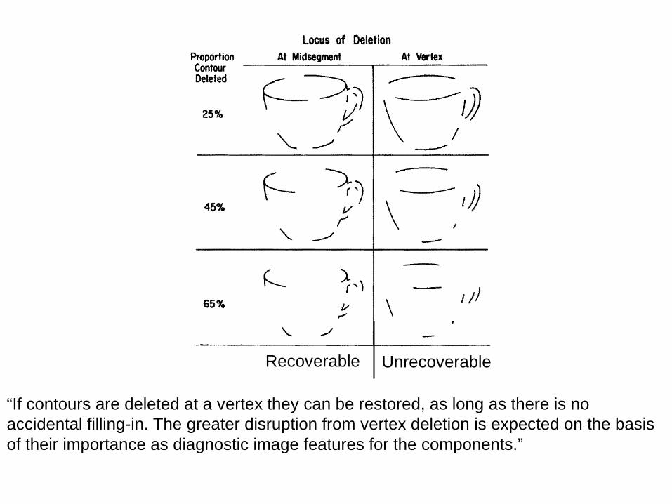
“If contours are deleted at a vertex they can be restored, as long as there is no accidental filling-in. The greater disruption from vertex deletion is expected on the basis of their importance as diagnostic image features for the components.”
Recoverable Unrecoverable
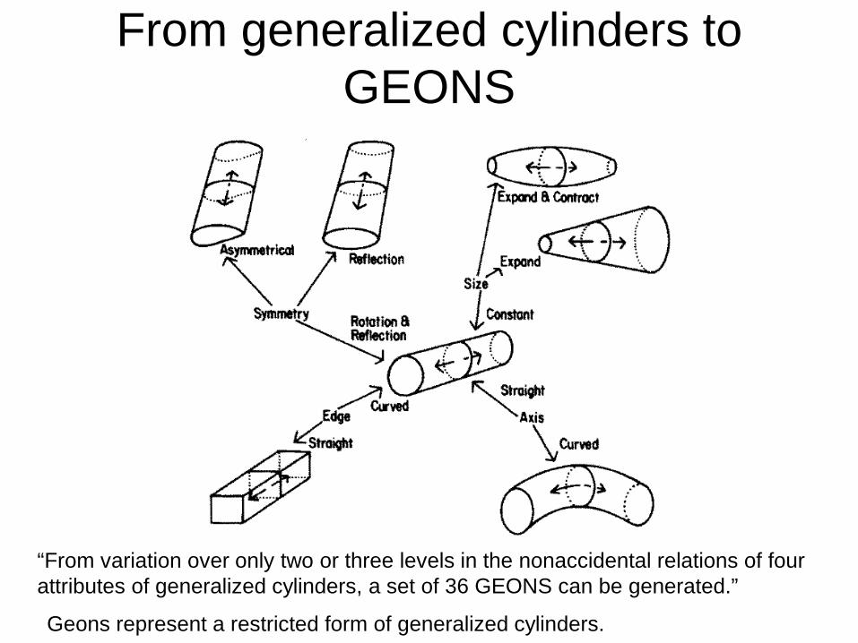
From generalized cylinders to GEONS
“From variation over only two or three levels in the nonaccidental relations of four attributes of generalized cylinders, a set of 36 GEONS can be generated.”
Geons represent a restricted form of generalized cylinders.
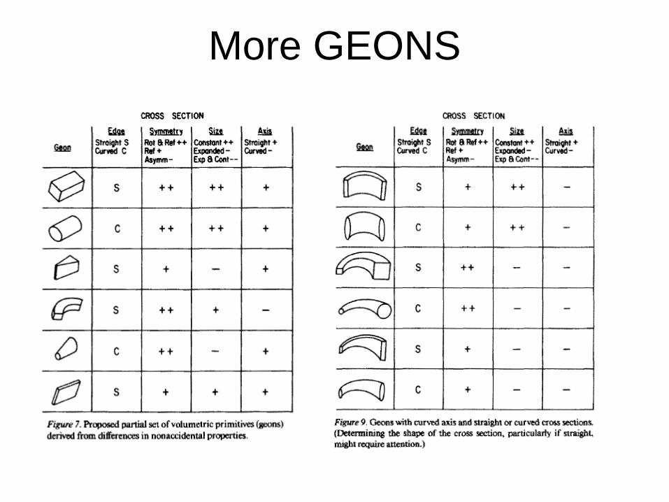
More GEONS

Objects and their geons
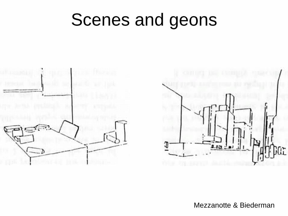
Scenes and geons
Mezzanotte & Biederman
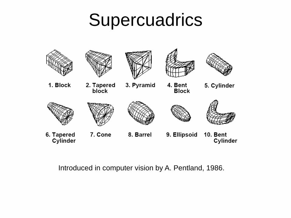
Supercuadrics
Introduced in computer vision by A. Pentland, 1986.
What is missing?
The notion of geometric structure. Although they were aware of it, the previous
works put more emphasis on defining the primitive elements than modeling their geometric relationships.
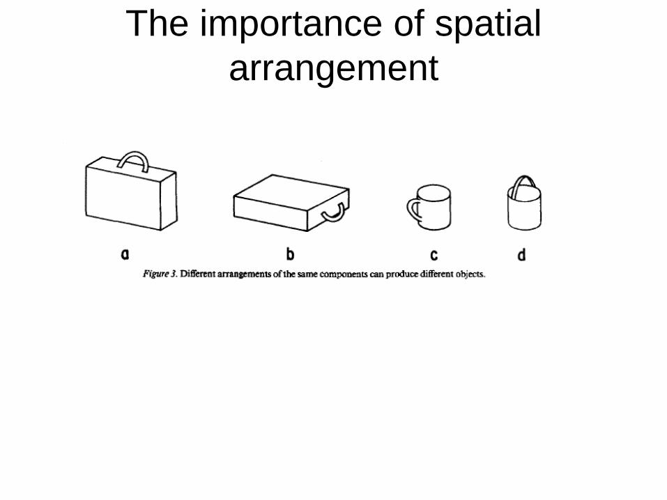
The importance of spatial arrangement

Parts and Structure approaches With a different perspective, these models focused more on the
geometry than on defining the constituent elements: • Fischler & Elschlager 1973 • Yuille ‘91 • Brunelli & Poggio ‘93 • Lades, v.d. Malsburg et al. ‘93 • Cootes, Lanitis, Taylor et al. ‘95 • Amit & Geman ‘95, ‘99 • Perona et al. ‘95, ‘96, ’98, ’00, ’03, ‘04, ‘05 • Felzenszwalb & Huttenlocher ’00, ’04 • Crandall & Huttenlocher ’05, ’06 • Leibe & Schiele ’03, ’04 • Many papers since 2000
Figure from [Fischler & Elschlager 73]

Representation • Object as set of parts
– Generative representation
• Model: – Relative locations between parts – Appearance of part
• Issues: – How to model location – How to represent appearance – Sparse or dense (pixels or regions) – How to handle occlusion/clutter
We will discuss these models more in depth later
But, despite promising initial results…things did not work out so well (lack of data, processing power, lack of reliable methods for low-level and mid-level vision)
Instead, a different way of thinking about object
detection started making some progress: learning based approaches and classifiers, which ignored low and mid-level vision.
Maybe the time is here to come back to some of
the earlier models, more grounded in intuitions about visual perception.

Neocognitron Fukushima (1980). Hierarchical multilayered neural network
S-cells work as feature-extracting cells. They resemble simple cells of the primary visual cortex in their response.
C-cells, which resembles complex cells in the visual cortex, are inserted in the network to allow for positional errors in the features of the stimulus. The input connections of C-cells, which come from S-cells of the preceding layer, are fixed and invariable. Each C-cell receives excitatory input connections from a group of S-cells that extract the same feature, but from slightly different positions. The C-cell responds if at least one of these S-cells yield an output.

Neocognitron
Learning is done greedily for each layer
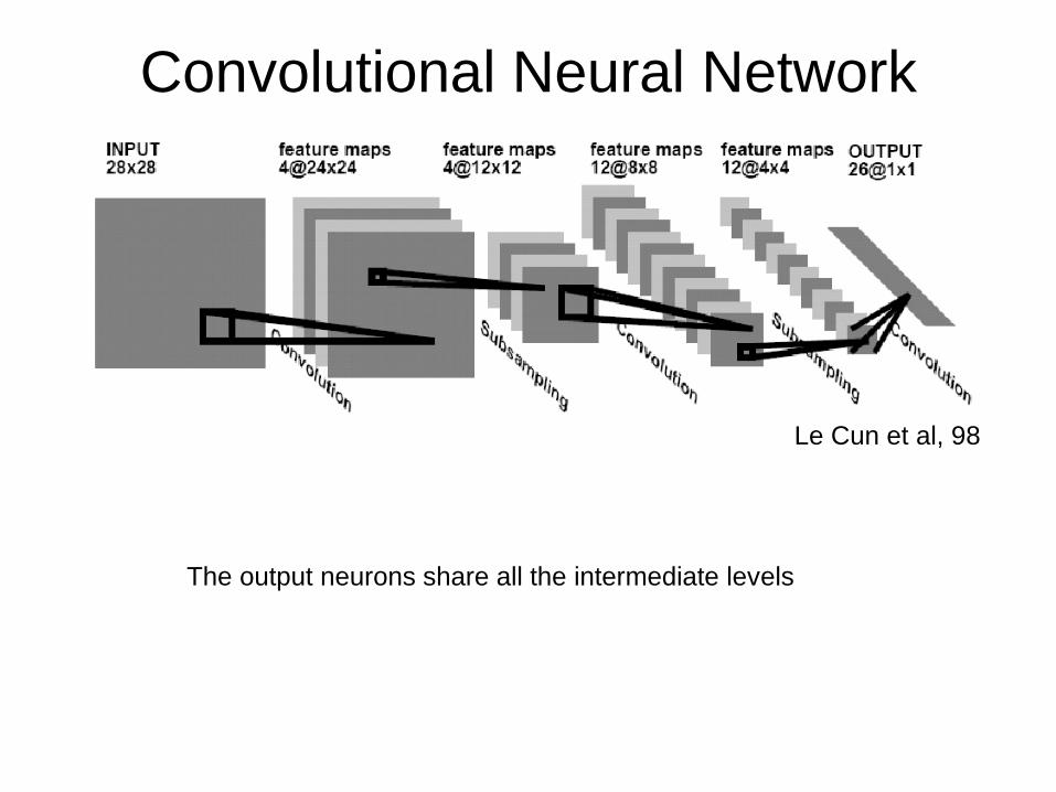
Convolutional Neural Network
The output neurons share all the intermediate levels
Le Cun et al, 98

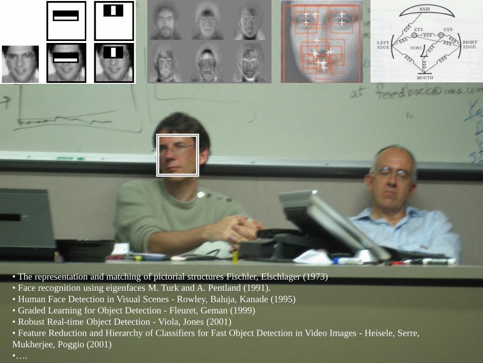
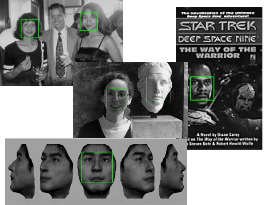
Face detection and the success of learning based approaches
• The representation and matching of pictorial structures Fischler, Elschlager (1973). • Face recognition using eigenfaces M. Turk and A. Pentland (1991). • Human Face Detection in Visual Scenes - Rowley, Baluja, Kanade (1995) • Graded Learning for Object Detection - Fleuret, Geman (1999) • Robust Real-time Object Detection - Viola, Jones (2001) • Feature Reduction and Hierarchy of Classifiers for Fast Object Detection in Video Images - Heisele, Serre, Mukherjee, Poggio (2001) •….
• The representation and matching of pictorial structures Fischler, Elschlager (1973). • Face recognition using eigenfaces M. Turk and A. Pentland (1991). • Human Face Detection in Visual Scenes - Rowley, Baluja, Kanade (1995) • Graded Learning for Object Detection - Fleuret, Geman (1999) • Robust Real-time Object Detection - Viola, Jones (2001) • Feature Reduction and Hierarchy of Classifiers for Fast Object Detection in Video Images - Heisele, Serre, Mukherjee, Poggio (2001) •….

Distribution-Based Face Detector
• Learn face and nonface models from examples [Sung and Poggio 95]
• Cluster and project the examples to a lower dimensional space using Gaussian distributions and PCA
• Detect faces using distance metric to face and nonface clusters

Distribution-Based Face Detector
• Learn face and nonface models from examples [Sung and Poggio 95]
Training Database 1000+ Real, 3000+ VIRTUAL
50,0000+ Non-Face Pattern

Neural Network-Based Face Detector • Train a set of multilayer perceptrons and
arbitrate a decision among all outputs [Rowley et al. 98]

Faces everywhere
60 http://www.marcofolio.net/imagedump/faces_everywhere_15_images_8_illusions.html
Paul Viola Michael J. Jones Mitsubishi Electric Research Laboratories (MERL)
Cambridge, MA
Most of this work was done at Compaq CRL before the authors moved to MERL
Rapid Object Detection Using a Boosted Cascade of Simple Features
http://citeseer.ist.psu.edu/cache/papers/cs/23183/http:zSzzSzwww.ai.mit.eduzSzpeoplezSzviolazSzresearchzSzpublicationszSzICCV01-Viola-Jones.pdf/viola01robust.pdf
Manuscript available on web:
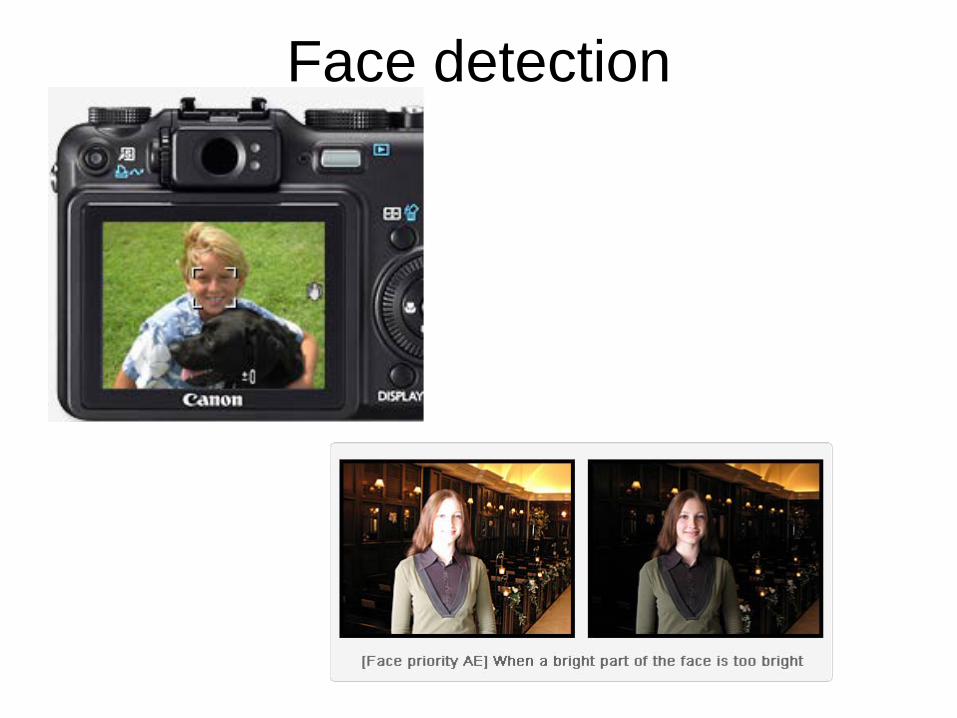
Face detection
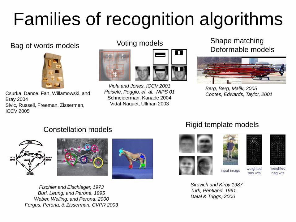
Families of recognition algorithms Bag of words models Voting models
Constellation models Rigid template models
Sirovich and Kirby 1987 Turk, Pentland, 1991 Dalal & Triggs, 2006
Fischler and Elschlager, 1973 Burl, Leung, and Perona, 1995
Weber, Welling, and Perona, 2000 Fergus, Perona, & Zisserman, CVPR 2003
Viola and Jones, ICCV 2001 Heisele, Poggio, et. al., NIPS 01
Schneiderman, Kanade 2004 Vidal-Naquet, Ullman 2003
Shape matching Deformable models
Csurka, Dance, Fan, Willamowski, and Bray 2004 Sivic, Russell, Freeman, Zisserman, ICCV 2005
Berg, Berg, Malik, 2005 Cootes, Edwards, Taylor, 2001

A simple object detector
• Simple but contains some of same basic elements of many state of the art detectors.
• Based on boosting which makes all the stages of the training and testing easy to understand.
Most of the slides are from the ICCV 05 short course http://people.csail.mit.edu/torralba/shortCourseRLOC/
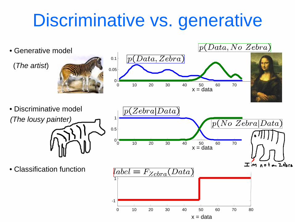
(The lousy painter)
Discriminative vs. generative
0 10 20 30 40 50 60 70 0
0.05
0.1
x = data
• Generative model
0 10 20 30 40 50 60 70 0
0.5
1
x = data
• Discriminative model
0 10 20 30 40 50 60 70 80
-1
1
x = data
• Classification function
(The artist)

Discriminative methods Object detection and recognition is formulated as a classification problem.
Bag of image patches
Decision boundary
… and a decision is taken at each window about if it contains a target object or not.
Computer screen
Background
In some feature space
Where are the screens?
The image is partitioned into a set of overlapping windows
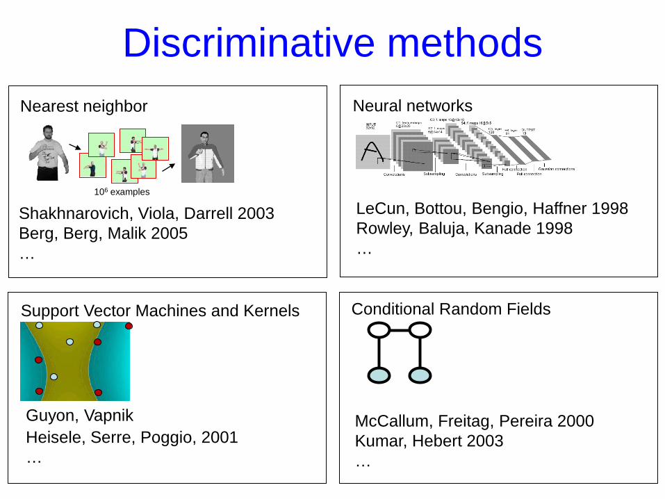
Discriminative methods
106 examples
Nearest neighbor
Shakhnarovich, Viola, Darrell 2003 Berg, Berg, Malik 2005 …
Neural networks
LeCun, Bottou, Bengio, Haffner 1998 Rowley, Baluja, Kanade 1998 …
Support Vector Machines and Kernels Conditional Random Fields
McCallum, Freitag, Pereira 2000 Kumar, Hebert 2003 …
Guyon, Vapnik Heisele, Serre, Poggio, 2001 …
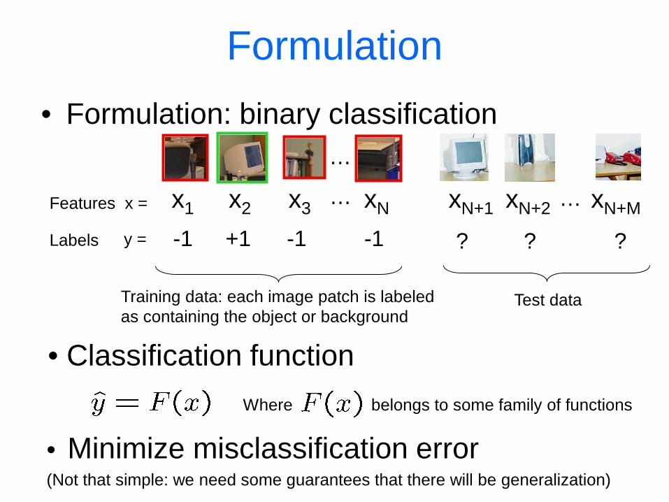
• Formulation: binary classification
Formulation
+1 -1
x1 x2 x3 xN
…
… xN+1 xN+2 xN+M
-1 -1 ? ? ?
…
Training data: each image patch is labeled as containing the object or background
Test data
Features x =
Labels y =
Where belongs to some family of functions
• Classification function
• Minimize misclassification error (Not that simple: we need some guarantees that there will be generalization)

Overview of section
• Object detection with classifiers
• Boosting – Gentle boosting – Weak detectors – Object model – Object detection
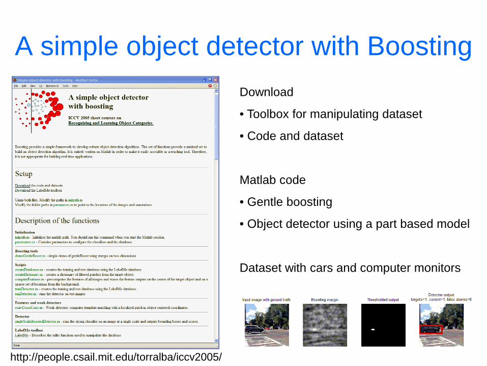
A simple object detector with Boosting Download
• Toolbox for manipulating dataset
• Code and dataset
Matlab code
• Gentle boosting
• Object detector using a part based model
Dataset with cars and computer monitors
http://people.csail.mit.edu/torralba/iccv2005/

• A simple algorithm for learning robust classifiers – Freund & Shapire, 1995 – Friedman, Hastie, Tibshhirani, 1998
• Provides efficient algorithm for sparse visual
feature selection – Tieu & Viola, 2000 – Viola & Jones, 2003
• Easy to implement, not requires external
optimization tools.
Why boosting?
For a description of several methods: Friedman, J. H., Hastie, T. and Tibshirani, R. Additive Logistic Regression: a Statistical View of Boosting. 1998
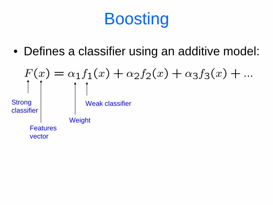
• Defines a classifier using an additive model:
Boosting
Strong classifier
Weak classifier
Weight Features vector
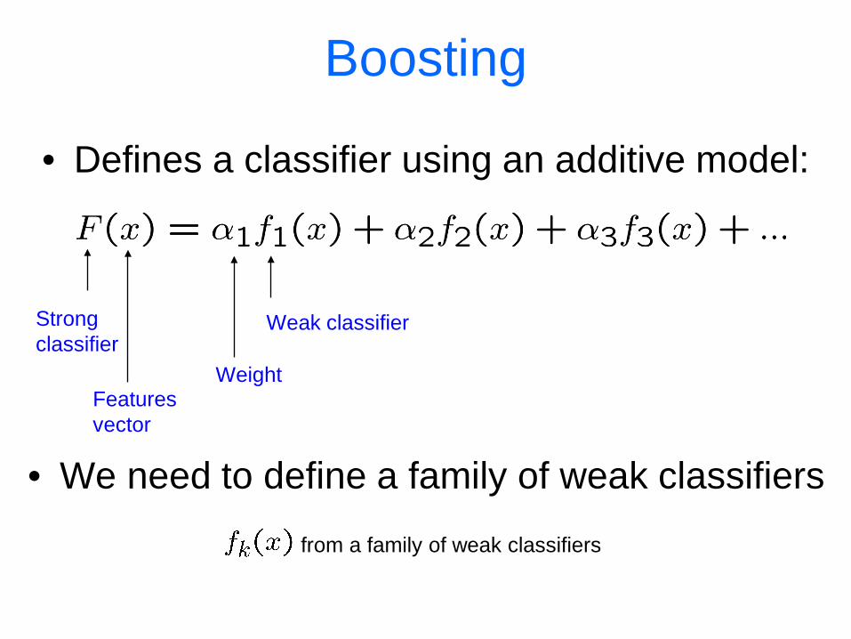
• Defines a classifier using an additive model:
• We need to define a family of weak classifiers
Boosting
Strong classifier
Weak classifier
Weight Features vector
from a family of weak classifiers
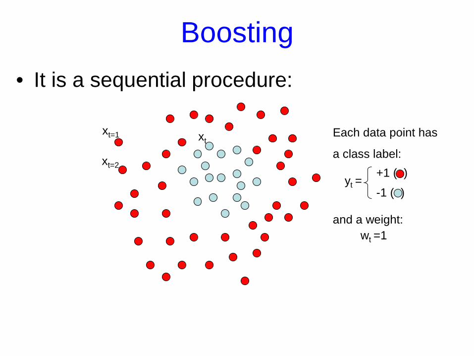
Each data point has
a class label:
wt =1 and a weight:
+1 ( )
-1 ( ) yt =
Boosting • It is a sequential procedure:
xt=1
xt=2
xt
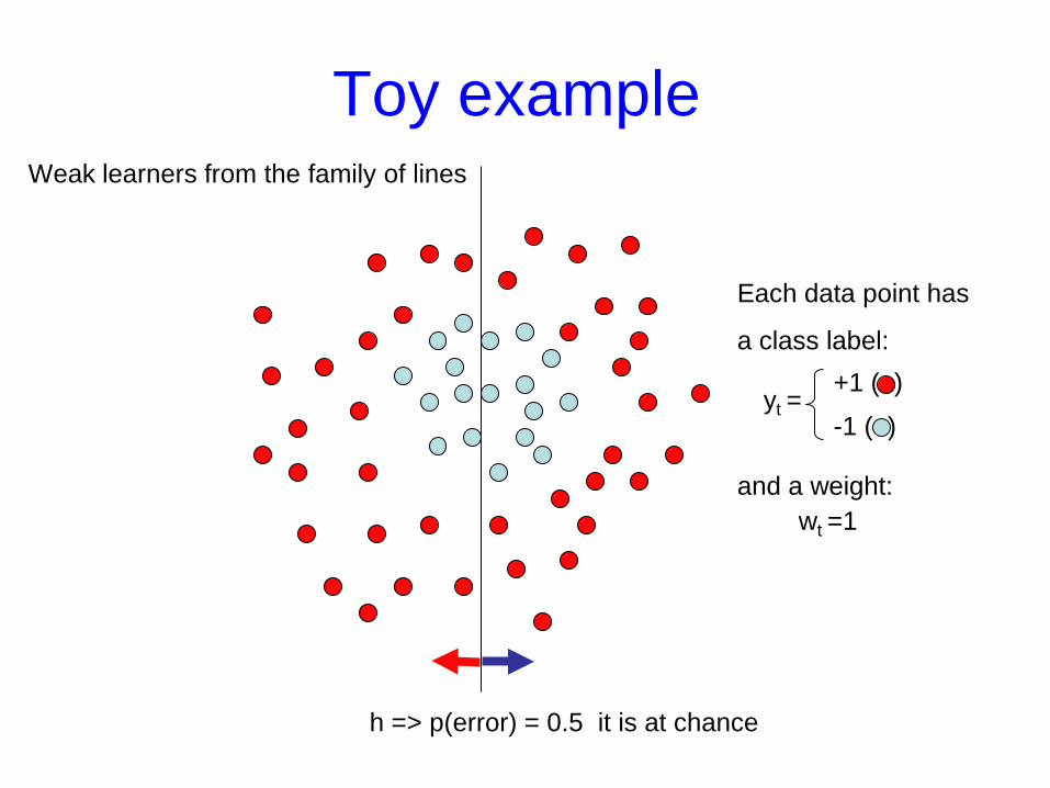
Toy example Weak learners from the family of lines
h => p(error) = 0.5 it is at chance
Each data point has
a class label:
wt =1 and a weight:
+1 ( )
-1 ( ) yt =

Toy example
This one seems to be the best
Each data point has
a class label:
wt =1 and a weight:
+1 ( )
-1 ( ) yt =
This is a ‘weak classifier’: It performs slightly better than chance.
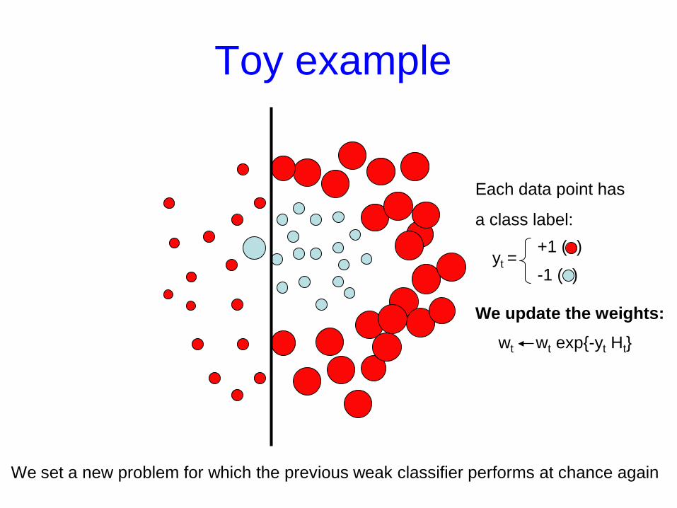
Toy example
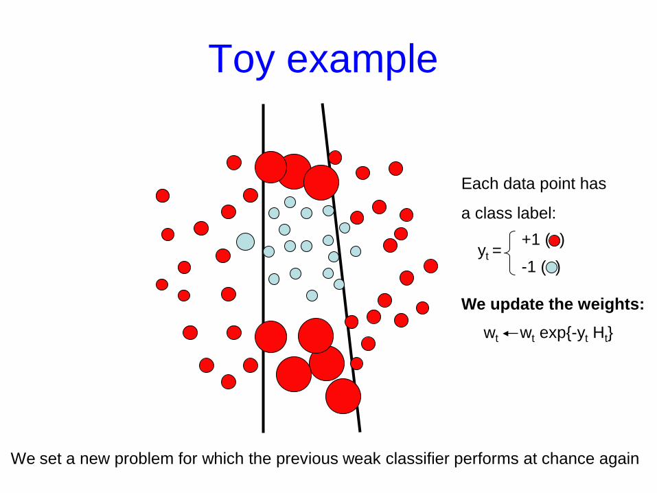
We set a new problem for which the previous weak classifier performs at chance again
Each data point has
a class label:
wt wt exp{-yt Ht}
We update the weights:
+1 ( )
-1 ( ) yt =

Toy example
We set a new problem for which the previous weak classifier performs at chance again
Each data point has
a class label:
wt wt exp{-yt Ht}
We update the weights:
+1 ( )
-1 ( ) yt =
Toy example
We set a new problem for which the previous weak classifier performs at chance again
Each data point has
a class label:
wt wt exp{-yt Ht}
We update the weights:
+1 ( )
-1 ( ) yt =

Toy example
We set a new problem for which the previous weak classifier performs at chance again
Each data point has
a class label:
wt wt exp{-yt Ht}
We update the weights:
+1 ( )
-1 ( ) yt =
Toy example
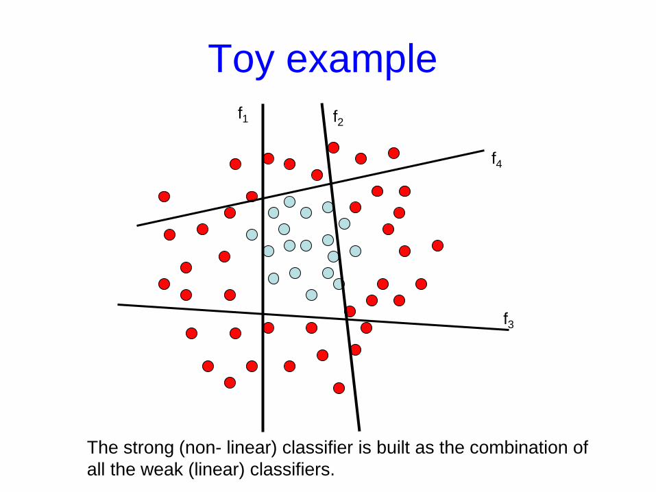
The strong (non- linear) classifier is built as the combination of all the weak (linear) classifiers.
f1 f2
f3
f4
Boosting
• Different cost functions and minimization algorithms result is various flavors of Boosting
• In this demo, I will use gentleBoosting: it is simple to implement and numerically stable.
Overview of section
• Object detection with classifiers
• Boosting – Gentle boosting – Weak detectors – Object model – Object detection

Boosting
Boosting fits the additive model
by minimizing the exponential loss
Training samples
The exponential loss is a differentiable upper bound to the misclassification error.
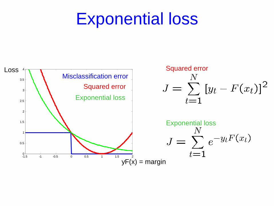
Exponential loss
-1.5 -1 -0.5 0 0.5 1 1.5 2 0
0.5
1
1.5
2
2.5
3
3.5
4 Squared error
Exponential loss
yF(x) = margin
Misclassification error Loss
Squared error Exponential loss
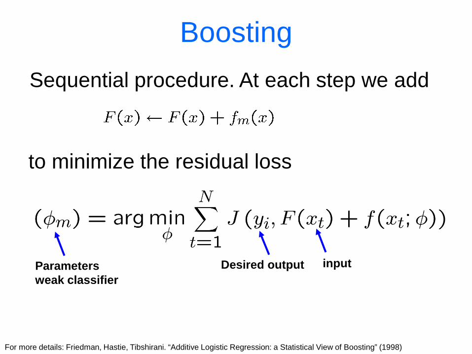
Boosting Sequential procedure. At each step we add
For more details: Friedman, Hastie, Tibshirani. “Additive Logistic Regression: a Statistical View of Boosting” (1998)
to minimize the residual loss input Desired output Parameters
weak classifier
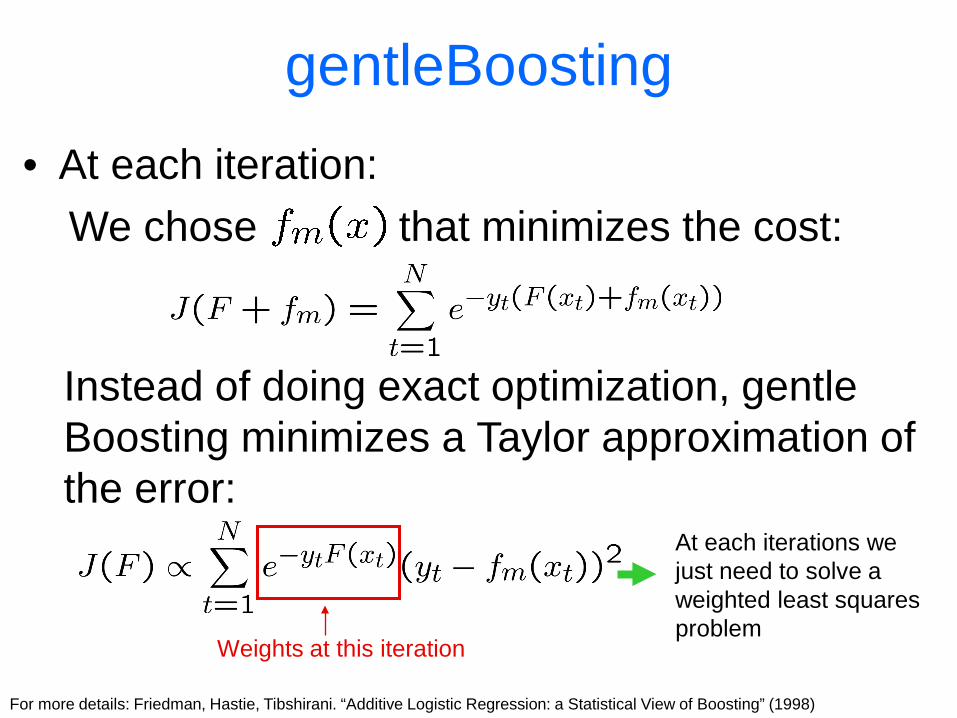
gentleBoosting
For more details: Friedman, Hastie, Tibshirani. “Additive Logistic Regression: a Statistical View of Boosting” (1998)
We chose that minimizes the cost:
At each iterations we just need to solve a weighted least squares problem
Weights at this iteration
• At each iteration:
Instead of doing exact optimization, gentle Boosting minimizes a Taylor approximation of the error:
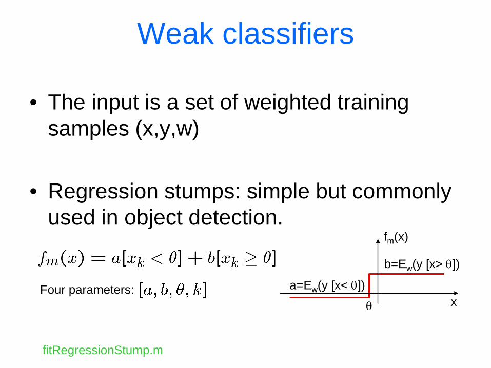
Weak classifiers
• The input is a set of weighted training samples (x,y,w)
• Regression stumps: simple but commonly used in object detection. Four parameters:
b=Ew(y [x> θ])
a=Ew(y [x< θ]) x
fm(x)
θ
fitRegressionStump.m

gentleBoosting.m
function classifier = gentleBoost(x, y, Nrounds) … for m = 1:Nrounds fm = selectBestWeakClassifier(x, y, w); w = w .* exp(- y .* fm); % store parameters of fm in classifier … end
Solve weighted least-squares
Re-weight training samples
Initialize weights w = 1

Demo gentleBoosting
> demoGentleBoost.m
Demo using Gentle boost and stumps with hand selected 2D data:
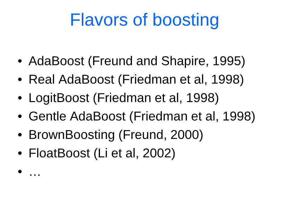
Flavors of boosting
• AdaBoost (Freund and Shapire, 1995) • Real AdaBoost (Friedman et al, 1998) • LogitBoost (Friedman et al, 1998) • Gentle AdaBoost (Friedman et al, 1998) • BrownBoosting (Freund, 2000) • FloatBoost (Li et al, 2002) • …

Overview of section
• Object detection with classifiers
• Boosting – Gentle boosting – Weak detectors – Object model – Object detection
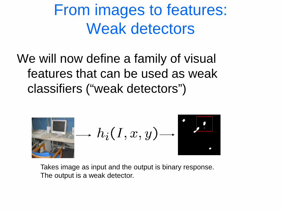
From images to features: Weak detectors
We will now define a family of visual features that can be used as weak classifiers (“weak detectors”)
Takes image as input and the output is binary response. The output is a weak detector.
Object recognition Is it really so hard?
Find the chair in this image
But what if we use smaller patches? Just a part of the chair?
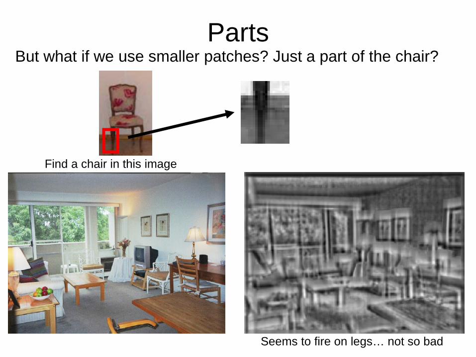
Parts
Find a chair in this image
But what if we use smaller patches? Just a part of the chair?
Seems to fire on legs… not so bad

Weak detectors Textures of textures Tieu and Viola, CVPR 2000. One of the first papers to use boosting for vision.
Every combination of three filters generates a different feature
This gives thousands of features. Boosting selects a sparse subset, so computations on test time are very efficient. Boosting also avoids overfitting to some extend.
Weak detectors
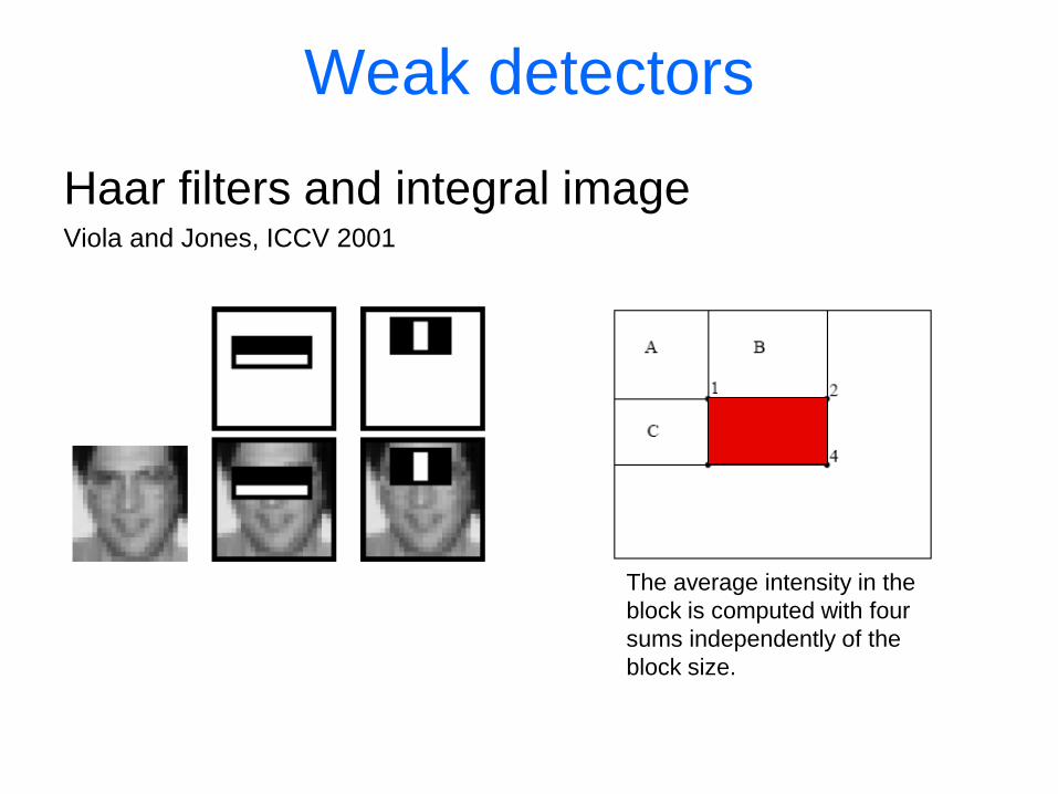
Haar filters and integral image Viola and Jones, ICCV 2001
The average intensity in the block is computed with four sums independently of the block size.
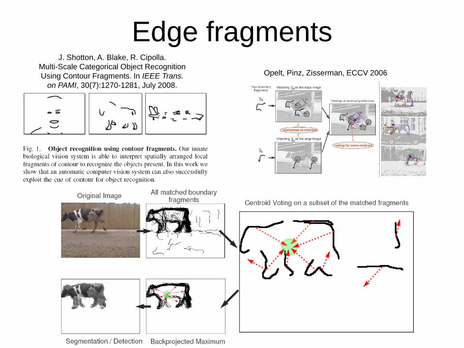
Edge fragments J. Shotton, A. Blake, R. Cipolla.
Multi-Scale Categorical Object Recognition Using Contour Fragments. In IEEE Trans.
on PAMI, 30(7):1270-1281, July 2008. Opelt, Pinz, Zisserman, ECCV 2006
Weak detectors
Other weak detectors: • Carmichael, Hebert 2004 • Yuille, Snow, Nitzbert, 1998 • Amit, Geman 1998 • Papageorgiou, Poggio, 2000 • Heisele, Serre, Poggio, 2001 • Agarwal, Awan, Roth, 2004 • Schneiderman, Kanade 2004 • …
Weak detectors
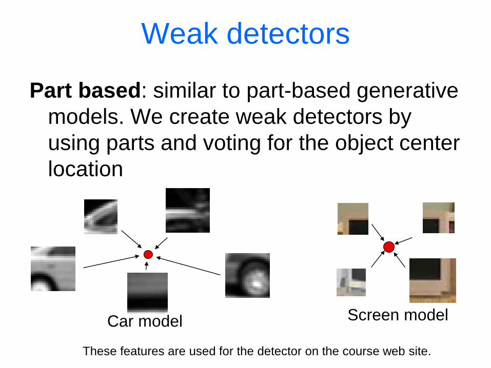
Part based: similar to part-based generative models. We create weak detectors by using parts and voting for the object center location
Car model Screen model
These features are used for the detector on the course web site.
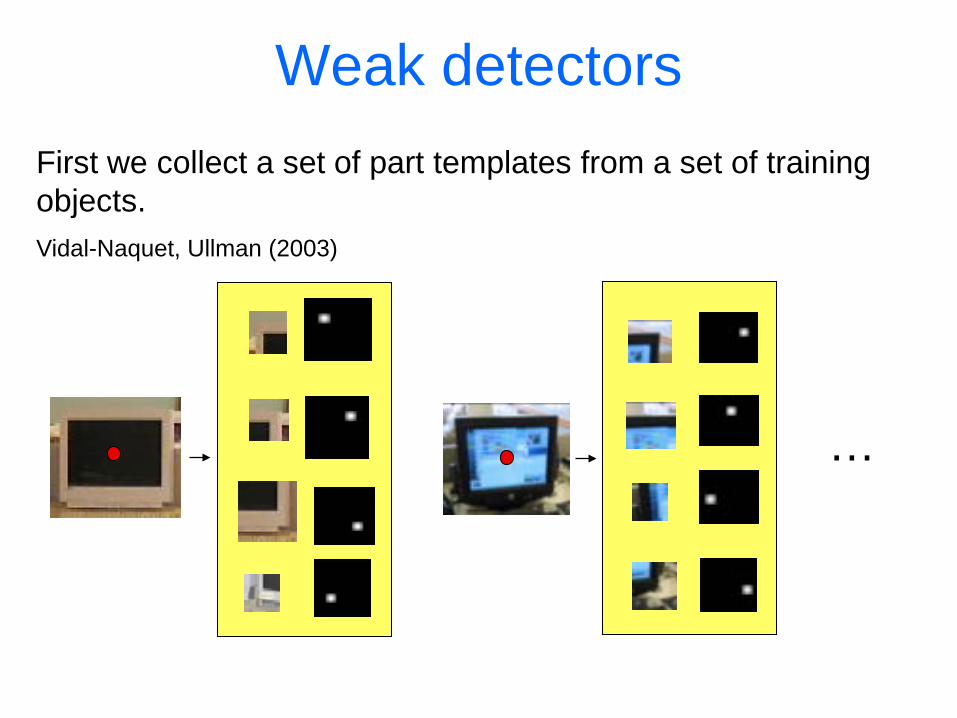
Weak detectors First we collect a set of part templates from a set of training objects. Vidal-Naquet, Ullman (2003)
…
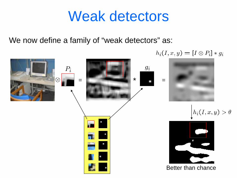
Weak detectors We now define a family of “weak detectors” as:
= =
Better than chance
*
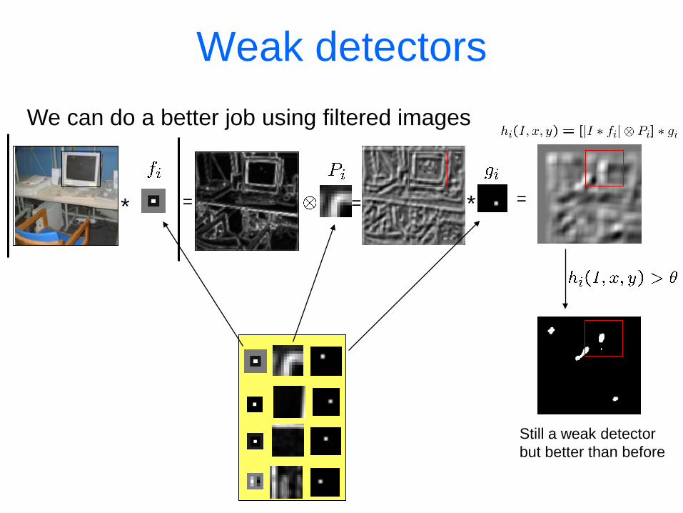
Weak detectors We can do a better job using filtered images
Still a weak detector but better than before
* * = = =
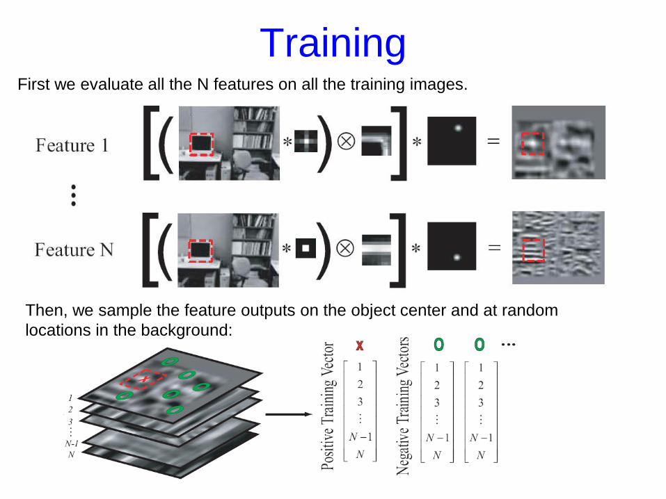
Training First we evaluate all the N features on all the training images.
Then, we sample the feature outputs on the object center and at random locations in the background:
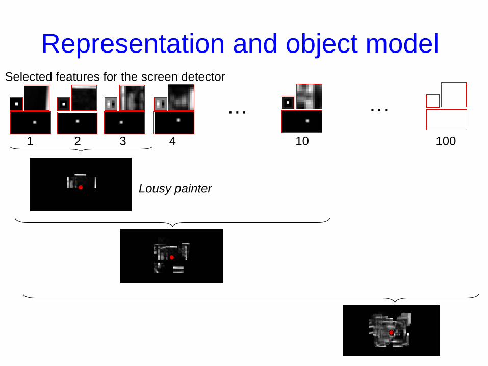
Representation and object model
… 4 10
Selected features for the screen detector
1 2 3
… 100
Lousy painter
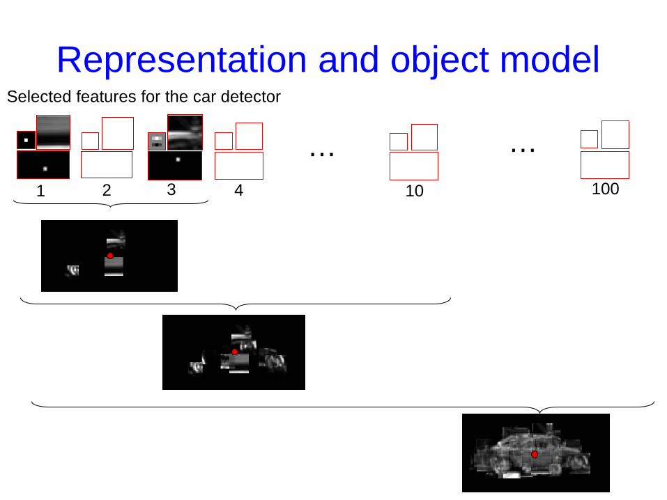
Representation and object model Selected features for the car detector
1 2 3 4 10 100
… …
Overview of section
• Object detection with classifiers
• Boosting – Gentle boosting – Weak detectors – Object model – Object detection
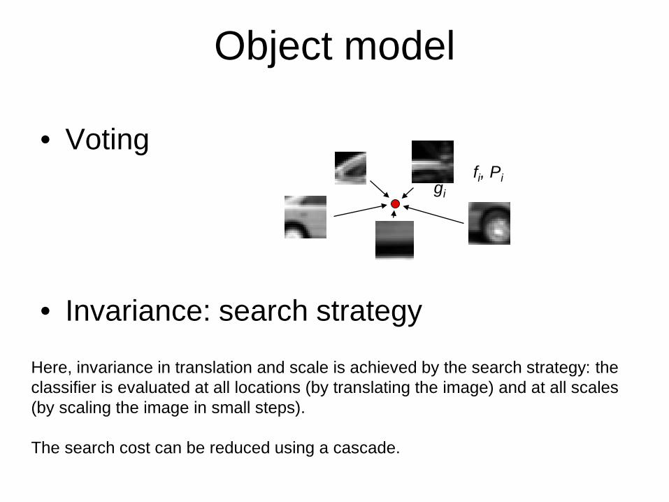
Object model
• Voting • Invariance: search strategy
fi, Pi gi
Here, invariance in translation and scale is achieved by the search strategy: the classifier is evaluated at all locations (by translating the image) and at all scales (by scaling the image in small steps). The search cost can be reduced using a cascade.
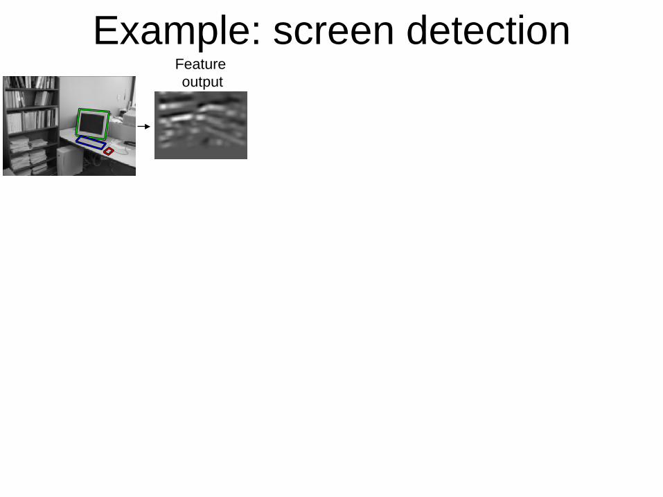
Example: screen detection Feature output
Example: screen detection Feature output
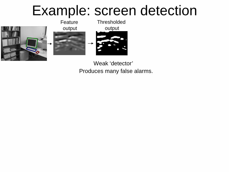
Thresholded output
Weak ‘detector’ Produces many false alarms.
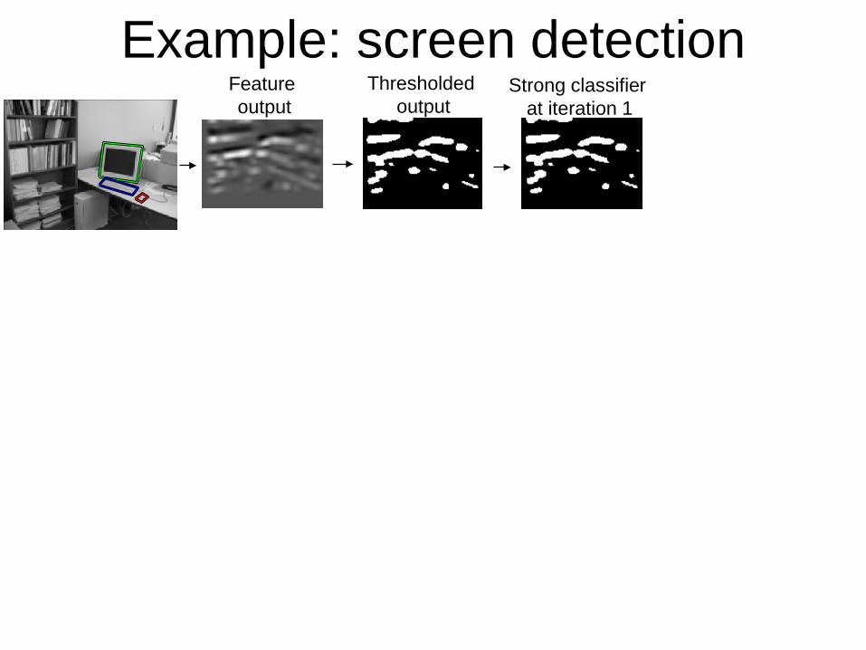
Example: screen detection Feature output
Thresholded output
Strong classifier at iteration 1

Example: screen detection Feature output
Thresholded output
Strong classifier
Second weak ‘detector’ Produces a different set of false alarms.
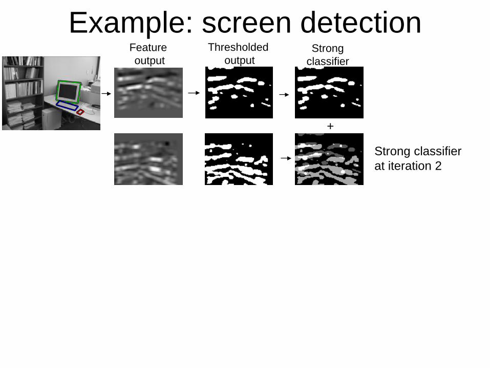
Example: screen detection
+
Feature output
Thresholded output
Strong classifier
Strong classifier at iteration 2
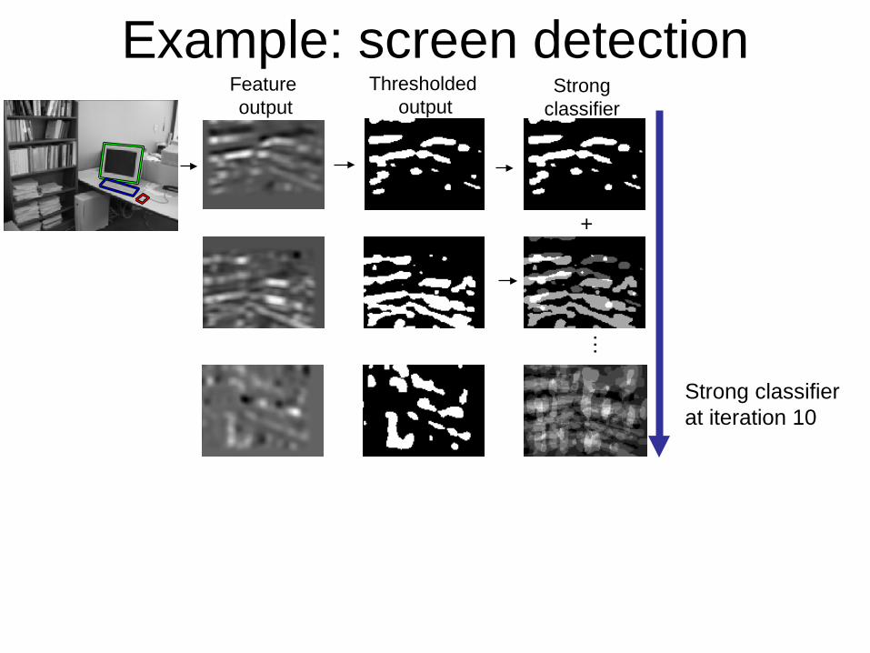
Example: screen detection
+
…
Feature output
Thresholded output
Strong classifier
Strong classifier at iteration 10
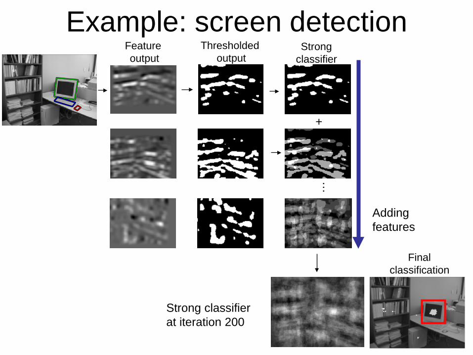
Example: screen detection
+
…
Feature output
Thresholded output
Strong classifier
Adding features
Final classification
Strong classifier at iteration 200
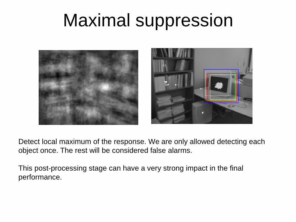
Maximal suppression
Detect local maximum of the response. We are only allowed detecting each object once. The rest will be considered false alarms. This post-processing stage can have a very strong impact in the final performance.
Related Documents