Lecture 2: Simple Mixtures 14-09-2010 • Aim of the lecture: Express chemical potential of the mixture in terms of its composition (molar fraction) • Lecture: – partial molar quantities – thermodynamics of mixing – ideal solutions – colligative properties – activities – Debye-Hückel limiting law – problems

Welcome message from author
This document is posted to help you gain knowledge. Please leave a comment to let me know what you think about it! Share it to your friends and learn new things together.
Transcript

Lecture 2: Simple Mixtures14-09-2010
• Aim of the lecture: Express chemical potential of the mixture in terms of its composition (molar fraction)
• Lecture:– partial molar quantities– thermodynamics of mixing– ideal solutions– colligative properties– activities– Debye-Hückel limiting law– problems

Partial molar quantities• we know how to describe phase equilibrium in the
case of a single substance. How it can be done in the case of mixtures?
• partial molar quantities: contribution of each component to the properties of mixturesour final goal is chemical potential, but let’s start with some simpler ones…
• Example: partial gas pressures (Dalton’s Law): The pressure exerted by mixture of gases if the sum of partial pressures of the gases.
...,A Bp p p= + + pxp ii = nnx ii /=and, where

Partial molar volume• How the total volume changes when
we change the amount of one of the components
• Observation: If we add say 18 cm3 of water to water the total volume increase will be exactly 18cm3, but if we add it to ethanol the increase would be just 14 cm3 . Partial molar volume depends on composition.
• Partial molar volume:
, ,
jj p T n
VVn
′
⎛ ⎞∂= ⎜ ⎟⎜ ⎟∂⎝ ⎠
Everything else is constant!

Partial molar volume
, ,
jj p T n
VVn
′
⎛ ⎞∂= ⎜ ⎟⎜ ⎟∂⎝ ⎠
Total volume
, , , ,B A
A B A A B BA Bp T n p T n
V VdV dn dn V dn V dnn n
⎛ ⎞ ⎛ ⎞∂ ∂= + = +⎜ ⎟ ⎜ ⎟∂ ∂⎝ ⎠ ⎝ ⎠
Volume change for a binary mixture:
the partial volume is a slope of the total volume graph vs. amount of moles.
A A B BV V n V n= +
number of moles of j
nA
nB
VHow we can calculate the total volume at a given concentration?- Let’s follow a path of constant cocentration:
can be negative
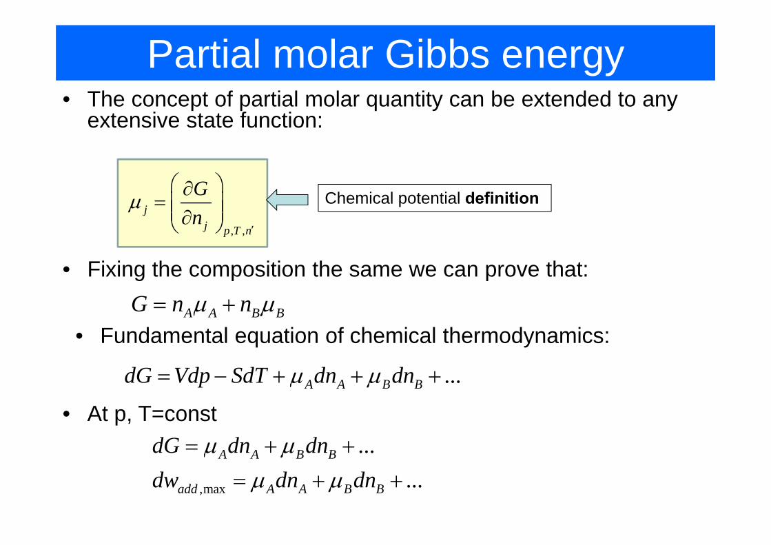
Partial molar Gibbs energy• The concept of partial molar quantity can be extended to any
extensive state function:
, ,
jj p T n
Gn
μ′
⎛ ⎞∂= ⎜ ⎟⎜ ⎟∂⎝ ⎠
A A B BG n nμ μ= +
...A A B BdG Vdp SdT dn dnμ μ= − + + +
• Fundamental equation of chemical thermodynamics:
,max
......
A A B B
add A A B B
dG dn dndw dn dn
μ μμ μ
= + += + +
• At p, T=const
Chemical potential definition
• Fixing the composition the same we can prove that:

Differential form of thermodynamic functions
H
j jj
dH TdS VdP dnμ= + +∑
G
j jj
dG SdT VdP dnμ= − + +∑
A
j jj
dA SdT PdV dnμ= − − +∑
U
j jj
dU TdS PdV dnμ= − +∑
TdSSdT−
VdPPdV−
, , ´
jj S V n
Un
μ⎛ ⎞∂
= ⎜ ⎟⎜ ⎟∂⎝ ⎠ , , ´
jj S P n
Hn
μ⎛ ⎞∂
= ⎜ ⎟⎜ ⎟∂⎝ ⎠
, , ´
jj T V n
An
μ⎛ ⎞∂
= ⎜ ⎟⎜ ⎟∂⎝ ⎠ , , ´
jj T P n
Gn
μ⎛ ⎞∂
= ⎜ ⎟⎜ ⎟∂⎝ ⎠
U G TS PV= + − j jj
dU TdS PdV dnμ= − +∑

Partial molar quantities• The Gibbs-Duhem equation
A A B B A A B BdG dn dn n d n dμ μ μ μ= + + +A A B BG n nμ μ= +
At P, T=const A A B BdG dn dnμ μ= +
Thus, as G is state function: 0A A B Bn d n dμ μ+ =
Gibbs-Duhemequation:
0J JJ
n dμ =∑
Let’s find change in Gibbs energy with infinitesimally change in composition:
The same is true for all partial molar quantities
Gibbs-Duhem equation shows that chemical potential of one compound cannot be changed indepentently of the other chemical potentials.
AB A
B
nd dn
μ μ= −

Thermodynamics of mixing• The Gibbs energy of mixing
Let’s consider mixing of 2 perfect gases at constant pressure p:
00ln pRT
pμ μ= +For each of them:
A A B BG n nμ μ= +and
After mixing the energy difference:
ln lnA Bmix A B
p pG n RT n RTp p
Δ = +
( ln ln )mix A A B BG nRT x x x xΔ = +
Using Dalton’s law:
,as 1, 0A B mixx G< Δ <

Thermodynamics of mixing• entropy of mixing
, ,
( ln ln )A B
mixmix A A B B
p n n
GS nR x x x xT
∂Δ⎛ ⎞Δ = − = − +⎜ ⎟∂⎝ ⎠
• enthalpy of mixing
0mix mixH G TdSΔ = Δ + =
The driving force of mixing is a purely entropic one!

Chemical potential of liquid• Ideal solutionsLet’s consider vapour (treated as perfect gas) above the solution. At equilibrium the chemical potential of a substance in vapour phase must be equal to its potential in the liquid phase
* 0 *lnA A ART pμ μ= +For pure substance:
0 lnA A ART pμ μ= +In solution:
* ln AA A
pRTp
μ μ= +
Raoult’s law: *A A Ap x p=
Mixtures obeying Raoult’s law called ideal solutions
Francouis Raoult experimentally found that:
* lnA A ART xμ μ= +

Chemical potential of liquid
' A Ak p kx=
rate of condensation
rate of evaporation
• Molecular interpretation of Raoult’s law
*
' and in case of pure liquid ( 1):
'
A A
A
A
kp xk
xkpk
=
=
=

Chemical potential of liquid
Similar liquidDissimilar liquid often show strong deviation

Chemical potential of liquid• Ideal-dilute solutions: Henry’s law
A A Ap x K=empirical constant, not the
vapour pressure
In a dilute solution the molecule of solvent are in an environment similar to a pure liquid while molecules of solute are not!

Chemical potential of liquid• Using Henry’s law
A A Ap x K=
Example: Estimate molar solubility of oxygen in water at 25 0C at a partial pressure of 21 kPa.
4 -14 -1
21kPa 2.9 10 mol kg7.9 10 kPa kg mol
AA
A
pxK
−= = = ××
molality
22 H O[O ] 0.29Ax mMρ= =

Colligative properties
• Elevation of boiling point• Depression of freezing point• Osmotic pressure phenomenon
All stem from lowering of the chemical potential of the solvent due to presence of solute (even in ideal solution!)
Larger

Colligative properties• Elevation of boiling point
* *( ) ( ) lnA A Ag l RT xμ μ= +**( ) ( )ln(1 ) vapA A
B
Gl gxRT RT
μ μ Δ−− = =
if liquid (solution) and vapour of pure A are in equilibrium:
* *21 1( )vap vap
B
H H TxR T T R T
Δ Δ Δ≈ − ≈
* *1 1ln(1 ) ( )vap
B
Hx
RT T TΔ
− = −
*2
Bvap
RTT xH
Δ =Δ
Let’s take derivative of both sides and apply Gibbs-Helmholtz equation:
2vapHG T
T RTΔΔ⎛ ⎞∂ ∂ =⎜ ⎟
⎝ ⎠
bT K bΔ =boiling constant
molality [mol/(kg solvent)]

Colligative properties• Depression of freezing point
* *( ) ( ) lnA A As l RT xμ μ= +
*2
Bvap
RTT xH
Δ =Δ
fT K bΔ =
Cryoscopic constant
Can be used to measure molar mass of a solute

Colligative properties• Dealing with boiling and cryoscopic constants
if we need to find boiling/freezing temperature change
- Calculate the molality of solute- Multiply by the relevant constant of solvent
can be also used to calculate molar mass

Colligative properties• Solubility
* *( ) ( ) lnB B Bs l RT xμ μ= +
**( ) ( )ln fusB BB
Gs lRT RT
μ μκ−Δ−
= =
fus fus fusG H T SΔ = Δ − Δ
*1 1ln ( )fus
B
Hx
R T TΔ
= −
*( ) * 0fus fus fusG T H T SΔ = Δ − Δ =

Colligative properties: Osmosis• Osmosis – spontaneous passage of pure solvent into solution
separated by semipermeable membrane
Van’t Hoff equation: [ ] , [ ] /BB RT B n VΠ = =molarity

Osmosis* *( ) ( ) lnA A Ap p RTμ μ κ= +Π +
**( ) ( )p
A A mp
p p V dpμ μ+Π
+Π = + ∫
For dilute solution: mRTx V= ΠB
/B An n/ AV n
More generally: [ ] (1 [ ] ...)B RT b BΠ = + +Osmotic virial coefficients
Van’t Hoff equation: [ ] , [ ] /BB RT B n VΠ = =
dG SdT Vdp= − +

Osmosis: Examples
• Calculate osmotic pressure exhibited by 0.1M solutions of mannitol and NaCl.
Mannitol (C6H8(OH)6)[ ] , [ ] /BB RT B n VΠ = =

Osmosis: Examples
Isotonic conditions
Hypotonic conditions:cells burst and dyehaemolysis (for blood)
Internal osmotic pressure keeps the cell “inflated”
Hypertonic conditions:cells dry and dye

Application of Osmosis• Using osmometry to determine molar mass of a macromolecule
Osmotic pressure is measured at a series of mass concentrations c and a plot ofvs. c is used to determine molar mass.
/ cΠ
[ ] (1 [ ] ...)B RT b BΠ = + +
ghρ /c M
2 ...h RT bRT cc gM gMρ ρ= + +

Membrane potential
• Electrochemical potential
Fcyt
Fext0 ln[ ]j j j A j jz N e RT j z Fμ μ μ= + Φ = + + Φ
P-
P-
P-Na+
Na+ Na+
P-
P-
P-
Na+
Na+ Na+
0 0ln[ ] ln[ ]
[ ]ln[ ]
in in out outNa Na Na Na
out
in
RT Na z F RT Na z F
NaRTF Na
μ μ+ + + ++ +
+
+
+ + Φ = + + Φ
⎛ ⎞ΔΦ = ⎜ ⎟
⎝ ⎠
• Example: membrane potential
Na+ salt of a protein

Activities• the aim: to modify the equations to make them applicable to real solutions
* **ln A
A AA
pRTp
μ μ= +
Generally:vapour pressure of A above solution
vapour pressure of A above pure A
* * lnA A ART xμ μ= +
For ideal solution
(Raoult’s law)
For real solution* * lnA A ART aμ μ= + activity of A
* * ln lnA A A ART x RTμ μ γ= + +
activity coefficient of A
* ; as 1AA A A A
A
pa a x xp
= → →

Activities• Ideal-dilute solution: Henry’s law B B Bp K κ=
* * ** *ln ln lnB B
B B B BB B
p KRT RT RT xp p
μ μ μ= + = + +
* 0 lnB B BRT xμ μ= +0
Bμ
• Real solutes* 0 lnB B BRT aμ μ= + B
BB
paK
=

Example: Biological standard state
• Biological standard state: let’s define chemical potential of hydrogen at pH=70 ln
H H HRT aμ μ+ + += +
0 07 ln(10) 40 /H H H
RT kJ molμ μ μ+ + += − = −
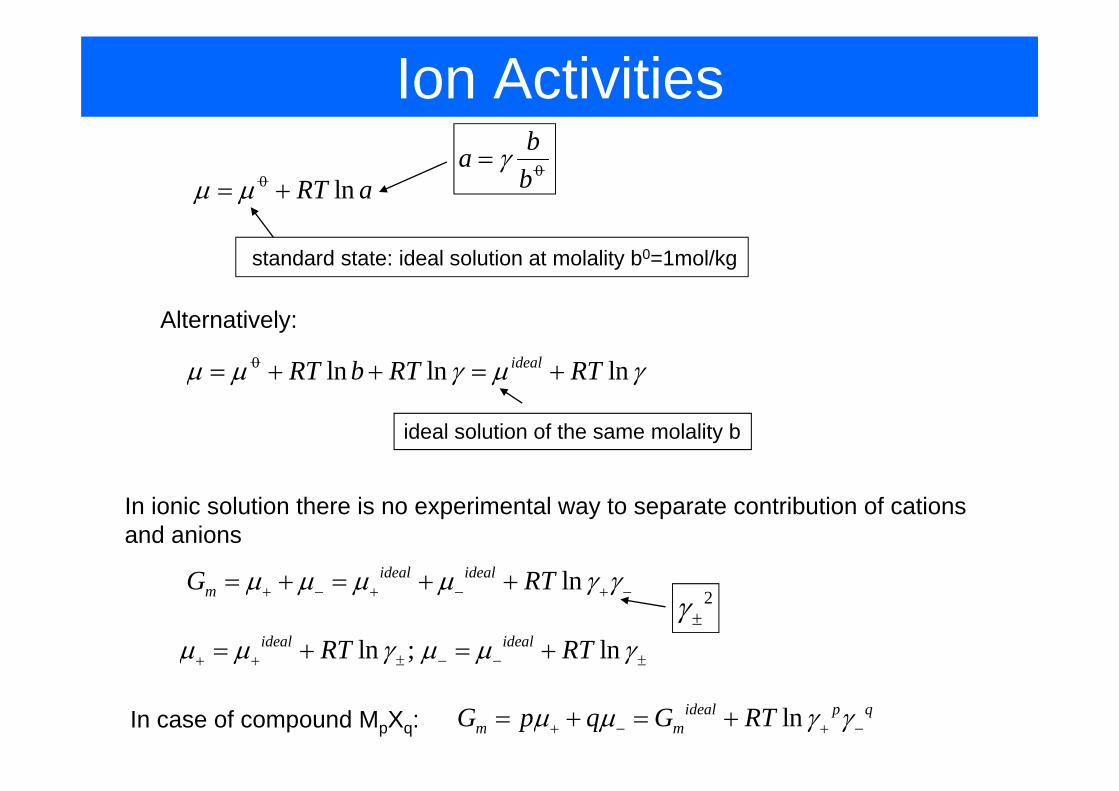
Ion Activities0 lnRT aμ μ= +
standard state: ideal solution at molality b0=1mol/kg
0
bab
γ=
0 ln ln lnidealRT b RT RTμ μ γ μ γ= + + = +
ideal solution of the same molality b
Alternatively:
In ionic solution there is no experimental way to separate contribution of cations and anions
lnideal idealmG RTμ μ μ μ γ γ+ − + − + −= + = + +
ln ; lnideal idealRT RTμ μ γ μ μ γ+ + ± − − ±= + = +
2γ ±
In case of compound MpXq: lnideal p qm mG p q G RTμ μ γ γ+ − + −= + = +

Debye-Hückel limiting law
• Coulomb interaction is the main reason for departing from ideality
• Oppositely charged ions attract each other and will form shells (ionic atmosphere) screening each other charge
• The energy of the screened ion is lowered as a result of interaction with its atmosphere

Debye-Hückel limiting law
12
2 0
log , 0.509 for water1where: ( / )2 i i
i
z z AI A
I z b b
γ ± + −= − = −
= ∑ Ionic strength of the solution
Example: calculate mean activity coefficient of 5 mM solution of KCL at 25C.
0 0 3
1 3 1/ 22
1 ( ) / / 5 102
log 0.509*(5 10 ) 0.0360.92
I b b b b b
z z AIγγ
−+ −
−± + −
±
= + = =
= − = − = −
=
i
i
In a limit of low concentration the activity coefficient can be calculated as:

Debye-Hückel limiting law
12log z z AIγ ± + −= −
12
12
log1
z z AI
BIγ + −± = −
+
Extended D-H law:

Problems (to solve in class)• 5.2a At 25°C, the density of a 50 per cent by mass ethanol–
water solution is 0.914 g cm–3. Given that the partial molar volume of water in the solution is 17.4 cm3 mol–1, calculate the partial molar volume of the ethanol
• 5.6a The addition of 100 g of a compound to 750 g of CCl4lowered the freezing point of the solvent by 10.5 K. Calculate the molar mass of the compound.
• 5.14a The osmotic pressure of solution of polystyrene in toluene were measured at 25 °C and the pressure was expressed in terms of the height of the solvent of density 1.004g/cm3. Calculate the molar mass of polystyrene:c [g/dm3] 2.042 6.613 9.521 12.602 h [cm] 0.592 1.910 2.750 3.600
• 5.20(a) Estimate the mean ionic activity coefficient and activity of a solution that is 0.010 mol kg–1 CaCl2(aq) and 0.030 mol kg–1 NaF(aq).
Related Documents