Lecture 2 Interconnection Networks for Parallel Computers

Lecture 2Interconnection Networks for Parallel Computers

adapted from…

Ananth Grama, Anshul Gupta, George Karypis, and Vipin Kumar``Introduction to Parallel Computing'',

Addison Wesley, 2003

Interconnection Networks for Parallel Computers

• Interconnection networks carry data between processors and to memory.

• Interconnects are made of – switches and – links (wires, fiber).

• Interconnects are classified as static or dynamic. – Static networks consist of point-to-point communication links

among processing nodes and are also referred to as directnetworks.

– Dynamic networks are built using switches and communication links. Dynamic networks are also referred to as indirectnetworks.

Static and DynamicInterconnection Networks

Classification of interconnection networks: (a) a static network; and (b) a dynamic network.

Interconnection Networks

• Switches map a fixed number of inputs to outputs.

• The total number of ports on a switch is the degree of the switch.

• The cost of a switch grows as the square of the degree of the switch, the peripheral hardware linearly as the degree, and the packaging costs linearly as the number of pins.

Interconnection Networks: Network Interfaces

• Processors talk to the network via a network interface.

• The network interface may hang off the I/O bus or the memory bus.

• In a physical sense, this distinguishes a cluster from a tightly coupled multicomputer.

• The relative speeds of the I/O and memory buses impact the performance of the network.

Network Topologies

• A variety of network topologies have been proposed and implemented.

• These topologies tradeoff performance for cost.

• Commercial machines often implement hybrids of multiple topologies for reasons of packaging, cost, and available components.

Scalability

• scalability is the ability of a system, network, or process, – to handle growing amounts of work in a graceful manner or – its ability to be enlarged to accommodate that growth.

[ André B. Bondi, 'Characteristics of scalability and their impact on performance', Proceedings of the 2nd international workshop on Software and performance, Ottawa, Ontario, Canada, 2000, pages 195 - 203 ]

• For example, it can refer to the capability of a system to increase total throughput under an increased load when resources (typically hardware) are added.

Network Topologies: Buses

• Some of the simplest and earliest parallel machines used buses.

• All processors access a common bus for exchanging data.

• The distance between any two nodes is O(1) in a bus. The bus also provides a convenient broadcast media.

• However, the bandwidth of the shared bus is a major bottleneck.

• Typical bus based machines are limited to dozens of nodes. Sun Enterprise servers and Intel Pentium based shared-bus multiprocessors are examples of such architectures.

Network Topologies: Buses

Bus-based interconnects (a) with no local caches; (b) with local memory/caches.

Since much of the data accessed by processors is local to the processor, a local memory can improve the performance of bus-based machines.

Network Topologies: Crossbars

A completely non-blocking crossbar network connecting p processors to b memory banks.

A crossbar network uses an p×m grid of switches to connect p inputs to m outputs in a non-blocking manner.

Network Topologies: Crossbars

• The cost of a crossbar of p processors grows as O(p2).

• This is generally difficult to scale for large values of p.

• Examples of machines that employ crossbars include the Sun Ultra HPC 10000 and the Fujitsu VPP500.

Network Topologies: Multistage Networks

• Crossbars have excellent performance scalability but poor cost scalability.

• Buses have excellent cost scalability, but poor performance scalability.

• Multistage interconnects strike a compromise between these extremes.

Network Topologies: Multistage Networks

The schematic of a typical multistage interconnection network.

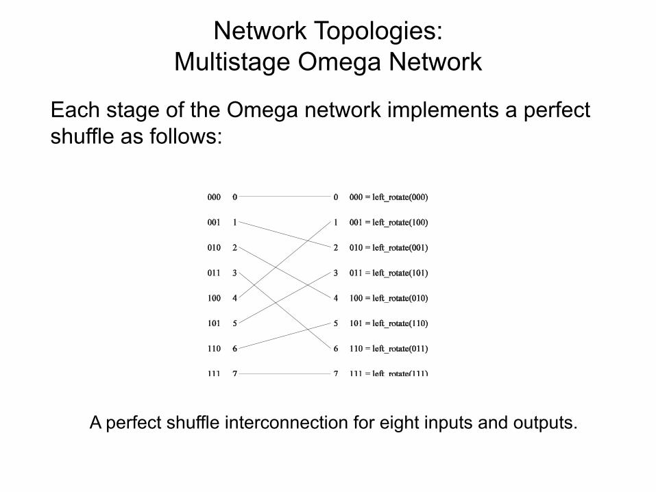
Network Topologies: Multistage Omega Network

• One of the most commonly used multistage interconnects is the Omega network.

• This network consists of log p stages, where p is the number of inputs/outputs.

• At each stage, input i is connected to output j if:

Network Topologies: Multistage Omega Network

Each stage of the Omega network implements a perfect shuffle as follows:

A perfect shuffle interconnection for eight inputs and outputs.

Network Topologies: Multistage Omega Network

• The perfect shuffle patterns are connected using 2×2 switches.• The switches operate in two modes – crossover or passthrough.

Two switching configurations of the 2 × 2 switch: (a) Pass-through; (b) Cross-over.

Network Topologies: Multistage Omega Network

A complete omega network connecting eight inputs and eight outputs.

An omega network has p/2 × log p switching nodes, and the cost of such a network grows as (p log p).

A complete Omega network with the perfect shuffle interconnects and switches can now be illustrated:

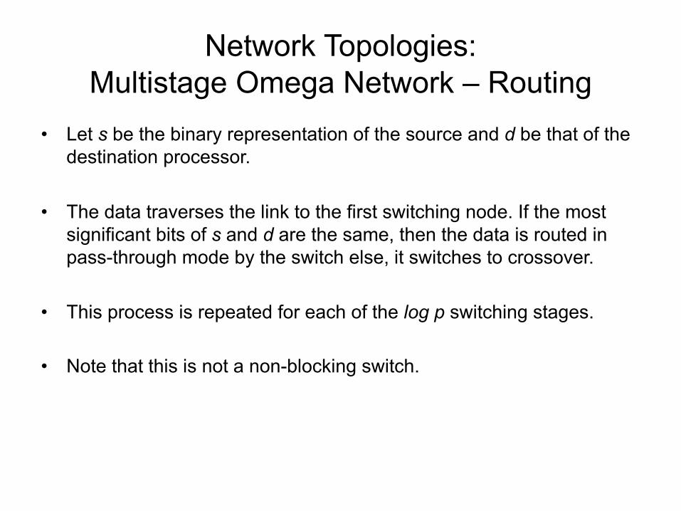
Network Topologies: Multistage Omega Network – Routing

• Let s be the binary representation of the source and d be that of the destination processor.

• The data traverses the link to the first switching node. If the most significant bits of s and d are the same, then the data is routed in pass-through mode by the switch else, it switches to crossover.

• This process is repeated for each of the log p switching stages.

• Note that this is not a non-blocking switch.

Network Topologies: Multistage Omega Network – Routing

An example of blocking in omega network: one of the messages (010 to 111 or 110 to 100) is blocked at link AB.

Static Interconnection Networks

Network Topologies: Completely Connected Network

• Each processor is connected to every other processor.

• The number of links in the network scales as O(p2).

• While the performance scales very well, the hardware complexity is not realizable for large values of p.

• In this sense, these networks are static counterparts of crossbars.

Network Topologies: Completely Connected and Star Connected Networks

Example of an 8-node completely connected network.

(a) A completely-connected network of eight nodes; (b) a star connected network of nine nodes.

Network Topologies: Star Connected Network

• Every node is connected only to a common node at the center.

• Distance between any pair of nodes is O(1). However, the central node becomes a bottleneck.

• In this sense, star connected networks are static counterparts of buses.

Network Topologies: Linear Arrays, Meshes, and k-d Meshes

• In a linear array, each node has two neighbors, one to its left and one to its right. If the nodes at either end are connected, we refer to it as a 1-D torus or a ring.

• A generalization to 2 dimensions has nodes with 4 neighbors, to the north, south, east, and west.

• A further generalization to d dimensions has nodes with 2dneighbors.

• A special case of a d-dimensional mesh is a hypercube. Here, d = log p, where p is the total number of nodes.

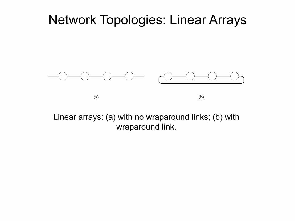
Network Topologies: Linear Arrays

Linear arrays: (a) with no wraparound links; (b) with wraparound link.

Network Topologies: Two- and Three Dimensional Meshes

Two and three dimensional meshes: (a) 2-D mesh with no wraparound; (b) 2-D mesh with wraparound link (2-D torus); and

(c) a 3-D mesh with no wraparound.

Network Topologies: Hypercubes and their Construction

Construction of hypercubes from hypercubes of lower dimension.

Network Topologies: Properties of Hypercubes

• The distance between any two nodes is at most log p.

• Each node has log p neighbors.

• The distance between two nodes is given by the number of bit positions at which the two nodes differ.

Network Topologies: Tree-Based Networks

Complete binary tree networks: (a) a static tree network; and (b) a dynamic tree network.

Network Topologies: Tree Properties

• The distance between any two nodes is no more than 2logp.

• Links higher up the tree potentially carry more traffic than those at the lower levels.

• For this reason, a variant called a fat-tree, fattens the links as we go up the tree.

• Trees can be laid out in 2D with no wire crossings. This is an attractive property of trees.

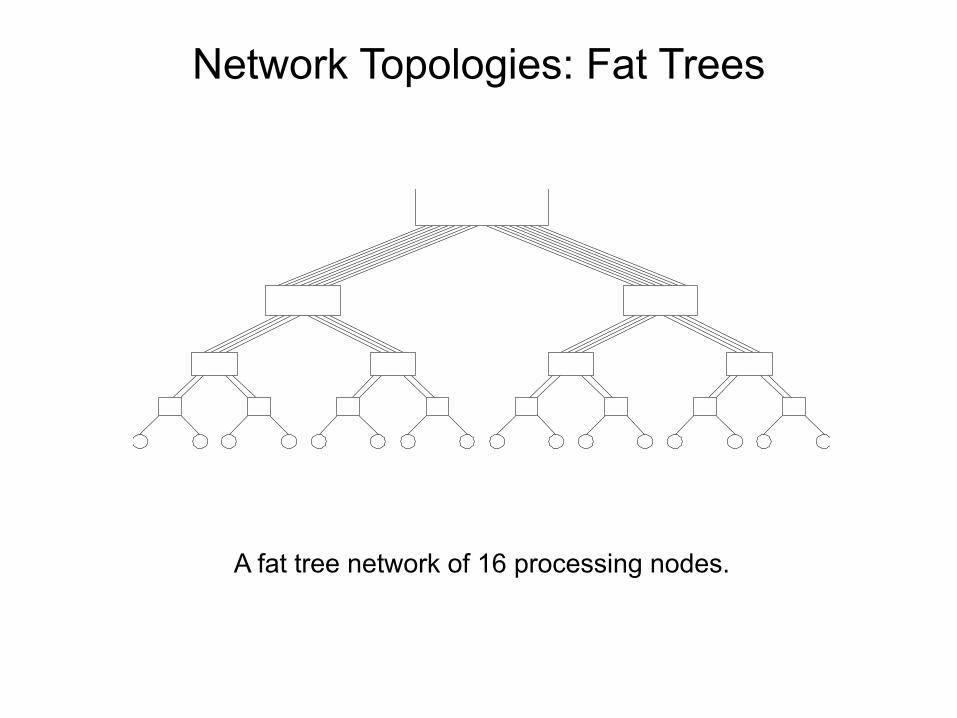
Network Topologies: Fat Trees

A fat tree network of 16 processing nodes.

Evaluating Static Interconnection Networks

• Diameter: The distance between the farthest two nodes in the network. The diameter of a linear array is p − 1, that of a mesh is 2( − 1), that of a tree and hypercube is log p, and that of a completely connected network is O(1).

• Bisection Width: The minimum number of wires you must cut to divide the network into two equal parts. The bisection width of a linear array and tree is 1, that of a mesh is , that of a hypercube is p/2 and that of a completely connected network is p2/4.

• Cost: The number of links or switches (whichever is asymptotically higher) is a meaningful measure of the cost. However, a number of other factors, such as the ability to layout the network, the length of wires, etc., also factor in to the cost.

Evaluating Static Interconnection Networks

Network Diameter BisectionWidth Arc Connectivity Cost

(No. of links)

Completely-connected

Star

Complete binary tree

Linear array

2-D mesh, no wraparound

2-D wraparound mesh

Hypercube

Wraparound k-ary d-cube

Evaluating Dynamic Interconnection Networks

Network Diameter Bisection Width

Arc Connectivity

Cost (No. of links)

Crossbar

Omega Network

Dynamic Tree

Cache Coherence in Multiprocessor Systems

• Interconnects provide basic mechanisms for data transfer.

• In the case of shared address space machines, additional hardware is required to coordinate access to data that might have multiple copies in the network.

• The underlying technique must provide some guarantees on the semantics.

• This guarantee is generally one of serializability, i.e., there exists some serial order of instruction execution that corresponds to the parallel schedule.

Cache coherenceIn computing, cache coherence (also cache coherency) refers to the consistency of data stored in local caches of a shared resource.

if the top client has a copy of a memory block from a previous read and the bottom client changes that memory block, the top client could be left with an invalid cache of memory without any notification of the change.

different protocols are used!

Communication Costs in Parallel Machines

• Along with idling and contention, communication is a major overhead in parallel programs.

• The cost of communication is dependent on a variety of features including the programming model semantics, the network topology, data handling and routing, and associated software protocols.

Message Passing Costs in Parallel Computers

• The total time to transfer a message over a network comprises of the following:– Startup time (ts): Time spent at sending and receiving nodes

(executing the routing algorithm, programming routers, etc.).

– Per-hop time (th): This time is a function of number of hops and includes factors such as switch latencies, network delays, etc.

– Per-word transfer time (tw): This time includes all overheads that are determined by the length of the message. This includes bandwidth of links, error checking and correction, etc.

Store-and-Forward Routing

• A message traversing multiple hops is completely received at an intermediate hop before being forwarded to the next hop.

• The total communication cost for a message of size m words to traverse l communication links is

• In most platforms, th is small and the above expression can be approximated by

Routing Techniques

Passing a message from node P0 to P3 (a) through a store-and-forward communication network; (b) and (c) extending the concept to cut-through

routing. The shaded regions represent the time that the message is in transit. The startup time associated with this message transfer is assumed

to be zero.

• Store-and-forward makes poor use of communication resources. • Packet routing breaks messages into packets and pipelines them

through the network. • Since packets may take different paths, each packet must carry

routing information, error checking, sequencing, and other related header information.

• The total communication time for packet routing is approximated by:

• The factor tw accounts for overheads in packet headers.

Packet Routing

Cut-Through Routing

• Takes the concept of packet routing to an extreme by further dividing messages into basic units called flits.

• Since flits are typically small, the header information must be minimized.

• This is done by forcing all flits to take the same path, in sequence. • A tracer message first programs all intermediate routers.

All flits then take the same route. • Error checks are performed on the entire message, as opposed to

flits. • No sequence numbers are needed.

Cut-Through Routing

• The total communication time for cut-through routing is approximated by:

• This is identical to packet routing, however, tw is typically much smaller.

Simplified Cost Model for Communicating Messages

• The cost of communicating a message between two nodes l hops away using cut-through routing is given by

• In this expression, th is typically smaller than ts and tw. For this reason, the second term does not show, particularly, when m is large.

• Furthermore, it is often not possible to control routing and placement of tasks.

• For these reasons, we can approximate the cost of message transfer by

Simplified Cost Model for Communicating Messages

• It is important to note that the original expression for communication time is valid for only uncongested networks.

• If a link takes multiple messages, the corresponding tw term must be scaled up by the number of messages.

• Different communication patterns congest different networks to varying extents.

• It is important to understand and account for this in the communication time accordingly.

Cost Models for Shared Address Space Machines

• While the basic messaging cost applies to these machines as well, a number of other factors make accurate cost modeling more difficult.

• Memory layout is typically determined by the system. • Finite cache sizes can result in cache thrashing. • Overheads associated with invalidate and update operations are

difficult to quantify. • Spatial locality is difficult to model. • Prefetching can play a role in reducing the overhead associated with

data access. • False sharing and contention are difficult to model.

Routing Mechanisms for Interconnection Networks

• How does one compute the route that a message takes from source to destination? – Routing must prevent deadlocks - for this reason, we use

dimension-ordered or e-cube routing. – Routing must avoid hot-spots - for this reason, two-step routing

is often used. In this case, a message from source s to destination d is first sent to a randomly chosen intermediate processor i and then forwarded to destination d.

Routing Mechanisms for Interconnection Networks

Routing a message from node Ps (010) to node Pd (111) in a three-dimensional hypercube using E-cube routing.

Mapping Techniques for Graphs

• Often, we need to embed a known communication pattern into a given interconnection topology.

• We may have an algorithm designed for one network, which we are porting to another topology.

For these reasons, it is useful to understand mapping between graphs.

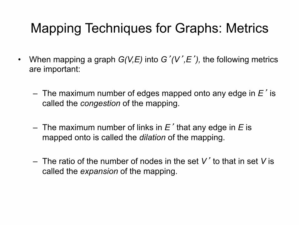
Mapping Techniques for Graphs: Metrics

• When mapping a graph G(V,E) into G’(V’,E’), the following metrics are important:

– The maximum number of edges mapped onto any edge in E’ is called the congestion of the mapping.

– The maximum number of links in E’ that any edge in E is mapped onto is called the dilation of the mapping.

– The ratio of the number of nodes in the set V’ to that in set V is called the expansion of the mapping.

Embedding a Linear Array into a Hypercube

• A linear array (or a ring) composed of 2d nodes (labeled 0 through 2d

− 1) can be embedded into a d-dimensional hypercube by mapping node i of the linear array onto node G(i, d) of the hypercube. The function G(i, x) is defined as follows:

0

Embedding a Linear Array into a Hypercube

The function G is called the binary reflected Gray code (RGC).

Since adjoining entries (G(i, d) and G(i + 1, d)) differ from each other at only one bit position, corresponding processors are mapped to neighbors in a hypercube. Therefore, the congestion, dilation, and expansion of the mapping are all 1.

Embedding a Linear Array into a Hypercube: Example

(a) A three-bit reflected Gray code ring; and (b) its embedding into a three-dimensional hypercube.

Embedding a Mesh into a Hypercube

• A 2r× 2s wraparound mesh can be mapped to a 2r+s-node hypercube by mapping node (i, j) of the mesh onto node G(i, r− 1) || G(j, s − 1) of the hypercube (where || denotes concatenation of the two Gray codes).

Embedding a Mesh into a Hypercube

(a) A 4 × 4 mesh illustrating the mapping of mesh nodes to the nodes in a four-dimensional hypercube; and (b) a 2 × 4 mesh embedded into

a three-dimensional hypercube.

Once again, the congestion, dilation, and expansion of the mapping is 1.

Embedding a Mesh into a Linear Array

• Since a mesh has more edges than a linear array, we will not have an optimal congestion/dilation mapping.

• We first examine the mapping of a linear array into a mesh and then invert this mapping.

• This gives us an optimal mapping (in terms of congestion).

Embedding a Mesh into a Linear Array: Example

(a) Embedding a 16 node linear array into a 2-D mesh; and (b) the inverse of the mapping. Solid lines correspond to links in the linear

array and normal lines to links in the mesh.

Embedding a Hypercube into a 2-D Mesh

• Each node subcube of the hypercube is mapped to a node row of the mesh.

• This is done by inverting the linear-array to hypercube mapping.• This can be shown to be an optimal mapping.

Embedding a Hypercube into a 2-D Mesh: Example

Embedding a hypercube into a 2-D mesh.

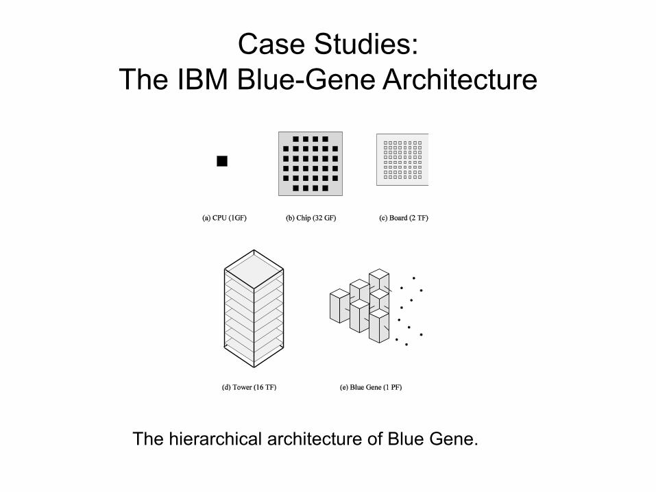
Case Studies: The IBM Blue-Gene Architecture

The hierarchical architecture of Blue Gene.

Case Studies: The Cray T3E Architecture

Interconnection network of the Cray T3E: (a) node architecture; (b) network topology.

Case Studies: The SGI Origin 3000 Architecture

Architecture of the SGI Origin 3000 family of servers.

Case Studies: The Sun HPC Server Architecture

Architecture of the Sun Enterprise family of servers.