Lecture 2

1

Lecture 2

ARMA models2012 International Finance

CYCU

2

White noise?• About color?• About sounds?

• Remember the statistical definition!

3

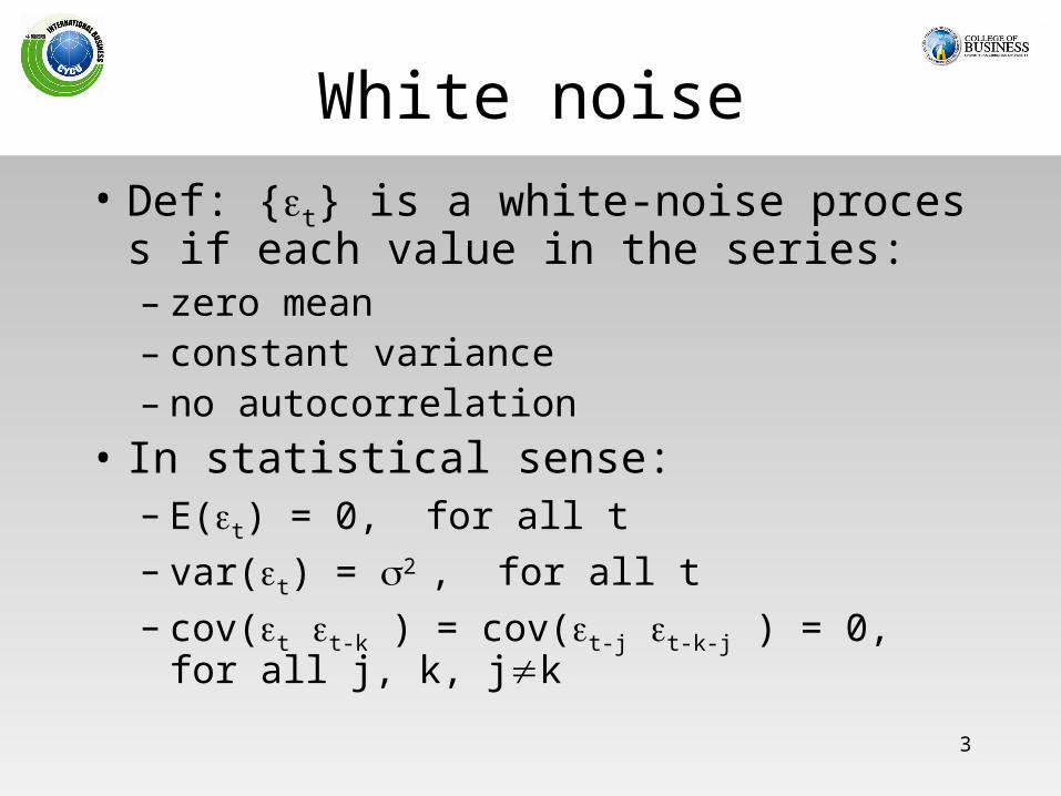
White noise• Def: {t} is a white-noise process if each val

ue in the series:– zero mean– constant variance– no autocorrelation

• In statistical sense:– E(t) = 0, for all t– var(t) = 2 , for all t– cov(t t-k ) = cov(t-j t-k-j ) = 0, for all j, k, jk

4

White noise• w.n. ~ iid (0, 2 )

iid: independently identical distribution

• white noise is a statistical “random” variable in time series

5

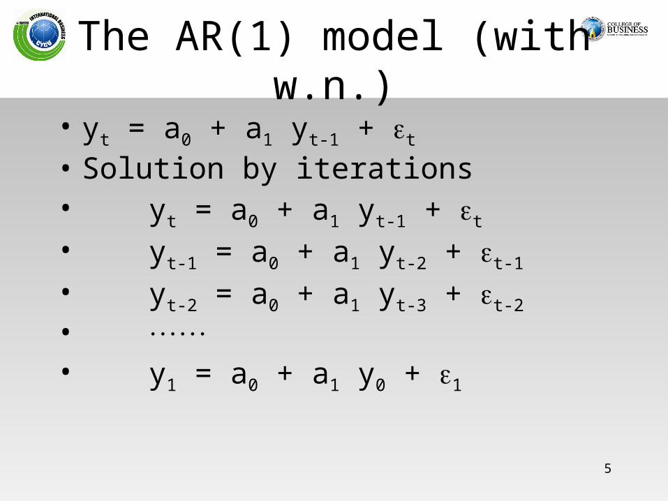
The AR(1) model (with w.n.)• yt = a0 + a1 yt-1 + t • Solution by iterations• yt = a0 + a1 yt-1 + t

• yt-1 = a0 + a1 yt-2 + t-1

• yt-2 = a0 + a1 yt-3 + t-2

• • y1 = a0 + a1 y0 + 1

6

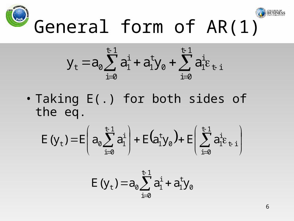
General form of AR(1)

• Taking E(.) for both sides of the eq.

it

1t

0i

i10

t1

1t

0i

i10t ayaaay

it

1t

0i

i10

t1

1t

0i

i10t aEyaEaaE)y(E

0t1

1t

0i

i10t yaaa)y(E

7

Compare AR(1) models• Math. AR(1)

0t

11

t1

0t y)a(a1a1ay

• “true” AR(1) in time series

0t

11

t1

0t y)a(a1a1a)yE(

8

Infinite population {yt}• If yt is an infinite DGP, E(yt) implies

constant) a :(note )a1(

aylim1

0tt

• Why? If |a1| < 1

0t

11

t1

0t y)a(a1a1ay

9

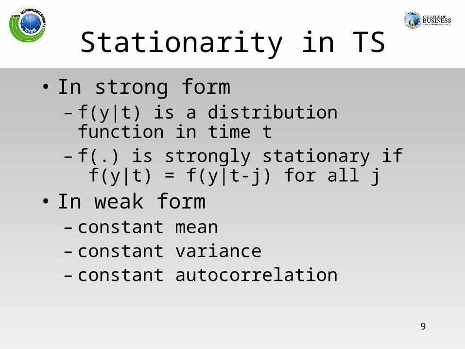
Stationarity in TS• In strong form

– f(y|t) is a distribution function in time t– f(.) is strongly stationary if

f(y|t) = f(y|t-j) for all j• In weak form

– constant mean– constant variance– constant autocorrelation

10

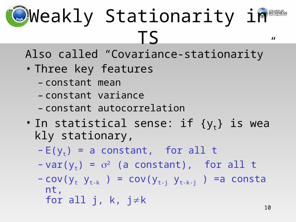
Weakly Stationarity in TSAlso called “Covariance-stationarity”• Three key features

– constant mean– constant variance– constant autocorrelation

• In statistical sense: if {yt} is weakly stationary, – E(yt) = a constant, for all t– var(yt) = 2 (a constant), for all t– cov(yt yt-k ) = cov(yt-j yt-k-j ) =a constant,

for all j, k, jk

11

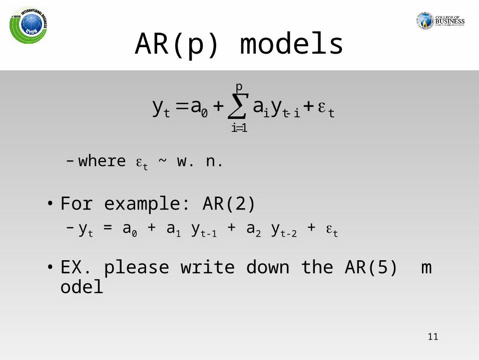
AR(p) models

– where t ~ w. n.

• For example: AR(2)– yt = a0 + a1 yt-1 + a2 yt-2 + t

• EX. please write down the AR(5) model

tit

p

1ii0t yaay

12

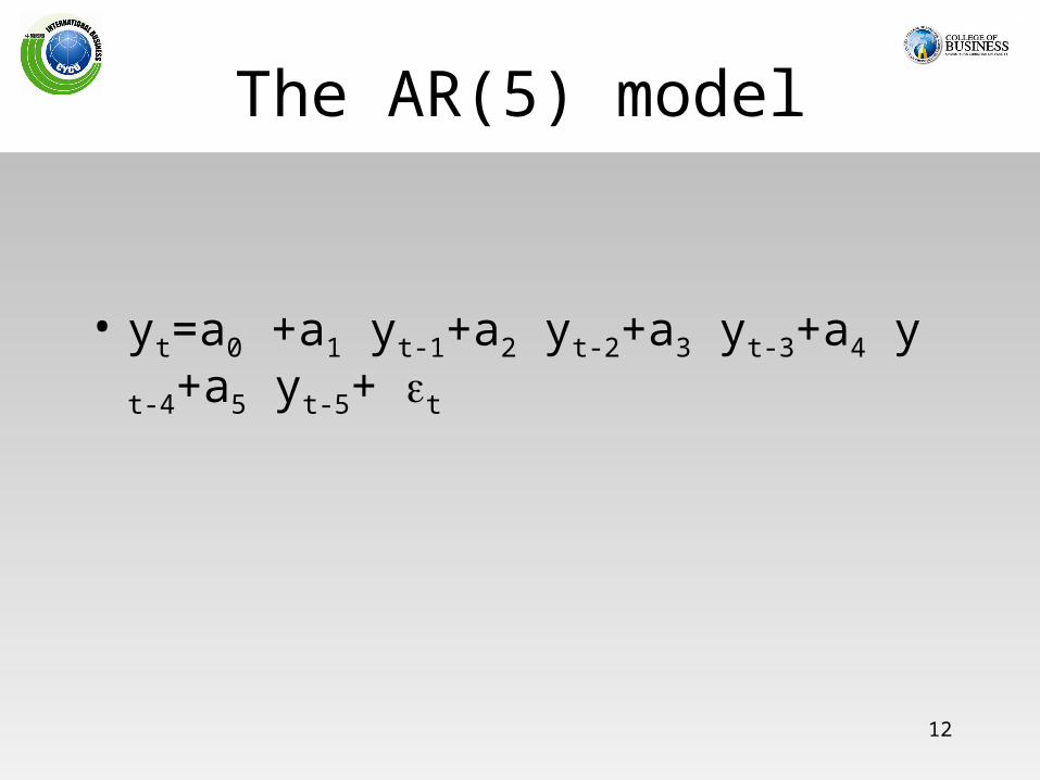
The AR(5) model

• yt=a0 +a1 yt-1+a2 yt-2+a3 yt-3+a4 yt-4+a5 yt-5+ t

13

Stationarity Restrictions for ARMA(p,q)

• Enders, p.60-61.• Sufficient condition

• Necessary condition

1|a|p

1ii

1ap

1ii

14

MA(q) models• MA: moving average

– the general form

it

q

1iit0t bay

– where t ~ w. n.

15

MA(q) models• MA(1)

1t1t0t bay

• Ex. Write down the MA(2) model...

16

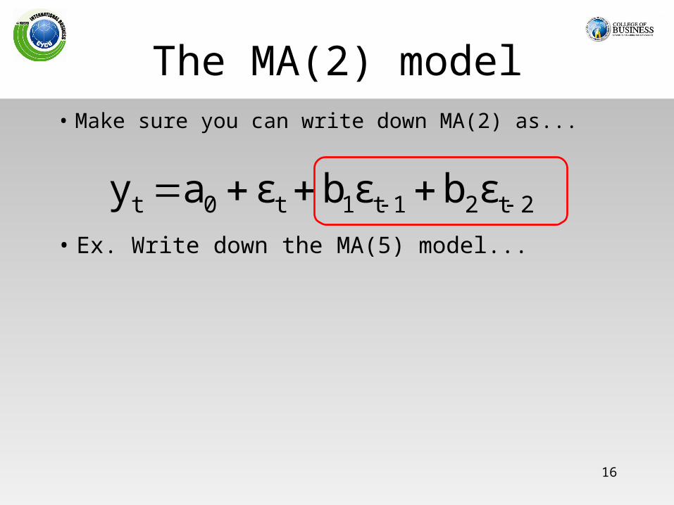
The MA(2) model• Make sure you can write down MA(2) as...

2t21t1t0t εbεbεay • Ex. Write down the MA(5) model...

17

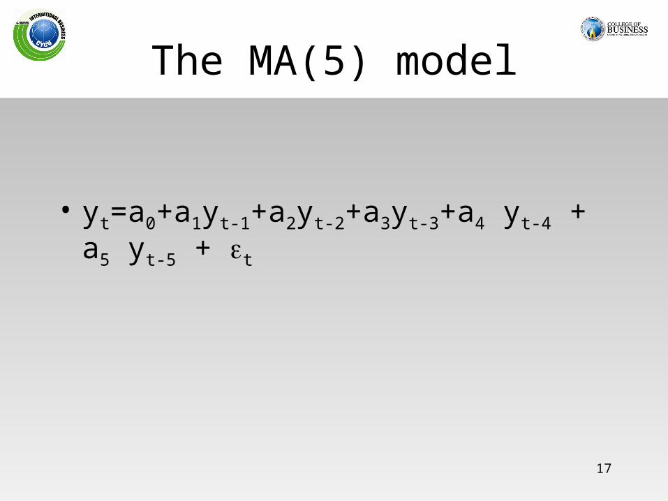
The MA(5) model

• yt=a0+a1yt-1+a2yt-2+a3yt-3+a4 yt-4 + a5 yt-5 + t

18

ARMA(p,q) models• ARMA=AR+MA, i.e.

– general form

• ARMA=AR+MA, i.e.– ARMA(1,1) = AR(1) + MA(1)

it

q

1iitit

p

1ii0t εbεyaay

itititi0t εbεyaay

19

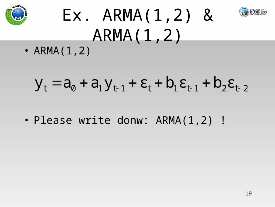
Ex. ARMA(1,2) & ARMA(1,2)• ARMA(1,2)

2t21t1t1t10t εbεbεyaay

• Please write donw: ARMA(1,2) !