Lecture 2

Sequential Ray Tracing

Lecture 2

Sequential Ray Tracing • Rays are traced through a pre-defined sequence of

surfaces while travelling from the object surface to the image surface.

• Rays hit each surface once in the order (sequence) in which the surfaces are defined. Particularly well-suited to imaging systems (including spectrometers).

• Numerically fast and extremely useful for the design, optimization and tolerancing of such systems.

• Aberrations evaluated using spot diagrams, ray fan plots, OPD plots, geometrical image analysis and MTF (physical optics) calculations.

February 19, 2015 Optical Systems Design 2

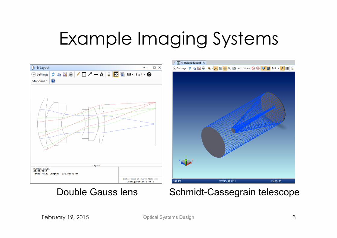
Example Imaging Systems

February 19, 2015 Optical Systems Design 3

Double Gauss lens Schmidt-Cassegrain telescope

Objectives: Lecture 2

At the end of this lecture you should: 1.  Be able to use ZEMAX to design and optimise a

simple singlet lens to specified parameters. 2.  Understand the use of meridional plane layouts,

spot diagrams, and ray fan plots to evaluate performance.

3.  Design and optimise a Cassegrain reflecting telescope to specified parameters.

4.  Understand the way that conic and higher order surfaces are specified in ZEMAX.

5.  Understand how to achromatise a doublet lens.

February 19, 2015 Optical Systems Design 4

Lens Data Editor (LDE) Surf: Type

the type of surface (Standard, Even Asphere, Diffraction Grating, etc)

  Comment an optional field for typing in surface specific comments

  Radius surface radius of curvature (the inverse of curvature) in lens units

  Thickness the thickness in lens units separating the vertex of the current surface to the vertex of the following surface

  Material the material type (glass, air, etc.) which separates the current surface and the next surface listed in the LDE

Coating any (anti-reflection) coating on surface

  Semi-Diameter the half-size of the surface in lens units

February 19, 2015 Optical Systems Design 5

Singlet Lens Parameters

•  Focal ratio is F/4. •  Glass is N-BK7. •  Effective focal length = 100mm. •  Field-Of-View = 10 degrees. •  Wavelength = 632.8nm (HeNe). •  Centre thickness of lens:  3mm to 12mm . •  Edge thickness of lens: minimum 2mm. •  Lens should be optimized for smallest RMS spot size

averaged over the field of view at the given wavelength.

•  Object is at infinity.

February 19, 2015 Optical Systems Design 6

System Settings

•  Entrance Pupil Diameter (EPD) is the diameter of the pupil in chosen lens units as seen from object space.

•  Effective focal length (efl) is distance along optical axis from the effective refracting surface (principal plane) to the paraxial focus.

•  So EPD = 25mm.

February 19, 2015 Optical Systems Design 7

System Explorer (Setup)

February 19, 2015 Optical Systems Design 8

Lens Data & Solves

February 19, 2015 Optical Systems Design 9

N.B. use of comments field

Optimize -> Quick Focus [Ctrl+Shift+Q]

Performance Evaluation (Analyze)

February 19, 2015 Optical Systems Design 10

Layout

Optical Path Difference

Spots

Ray Fan

Variables for Optimisation

•  Thickness of lens •  Front radius of curvature •  Back focal distance (from Surface 2 to

IMA plane)

February 19, 2015 Optical Systems Design 11

Optimize Wizard (Default Merit Function)

February 19, 2015 Optical Systems Design 12

Final System Results (Optimize)

February 19, 2015 Optical Systems Design 13

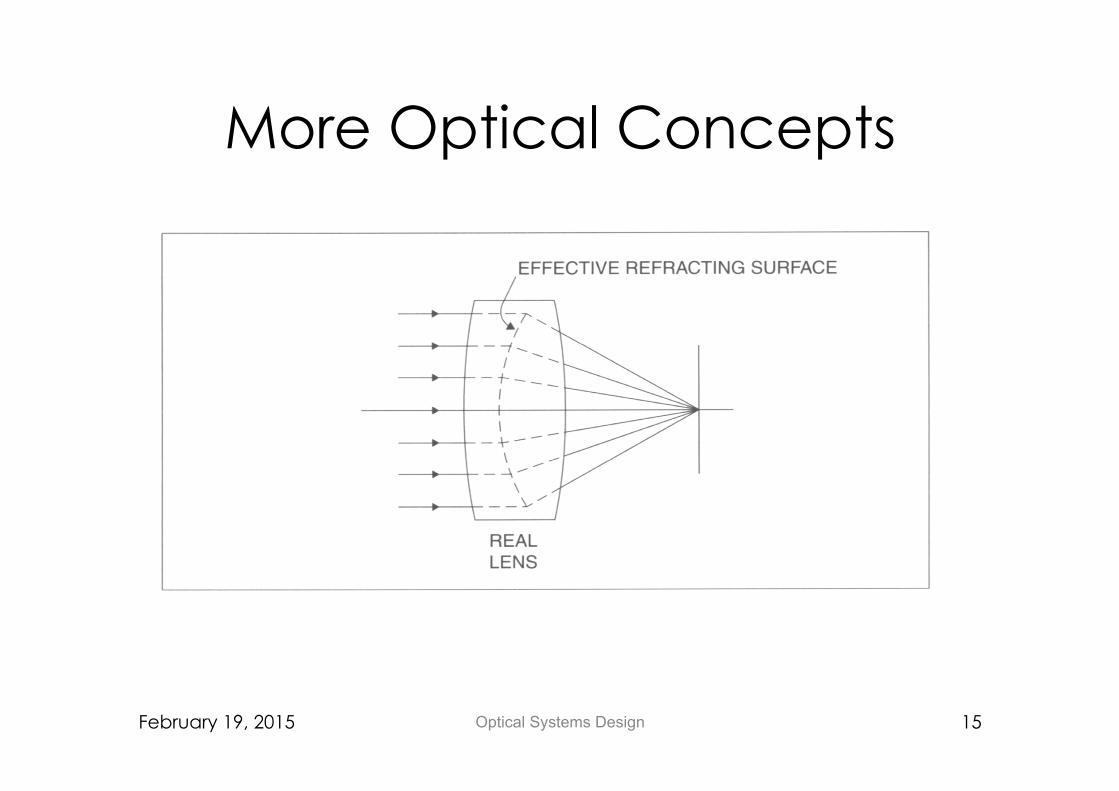
More Optical Concepts

•  Effective Refracting Surface –  Virtual surface at which entering and exiting rays meet.

A plane for paraxial (first order) rays close to the axis.

•  Zones –  Annular regions of constant distance from the optical

axis. Can apply to lens surfaces, stops, pupils, objects &

images. •  Paraxial rays

–  Rays close to the optical axis for which first order (linear) equations can be used for the ray transport calculations.

February 19, 2015 Optical Systems Design 14

More Optical Concepts

February 19, 2015 Optical Systems Design 15

Tangential & Sagittal Planes •  Tangential plane is identical to the

meridional plane for an axially symmetric system. Tangential rays lie within the tangential plane.

•  Sagittal plane is orthogonal to the tangential plane and intersects it along the chief ray. All sagittal rays are skew rays. The sagittal pane changes its tilt after each surface to follow the direction of the chief ray.

February 19, 2015 Optical Systems Design 16

Tangential & Sagittal Planes

February 19, 2015 Optical Systems Design 17

Back Focal Length & Effective Focal Length

•  Back focal length (BFL) is the distance along the optical axis from the vertex of the rear lens surface to the on-axis paraxial focus for an object at infinity.

•  Effective focal length (EFL) is the distance along the optical axis from the vertex of the effective refracting surface to the on-axis paraxial focus for an object at infinity.

•  BFL controls the longitudinal location of the focus •  EFL controls the transverse image scale at focus

February 19, 2015 Optical Systems Design 18

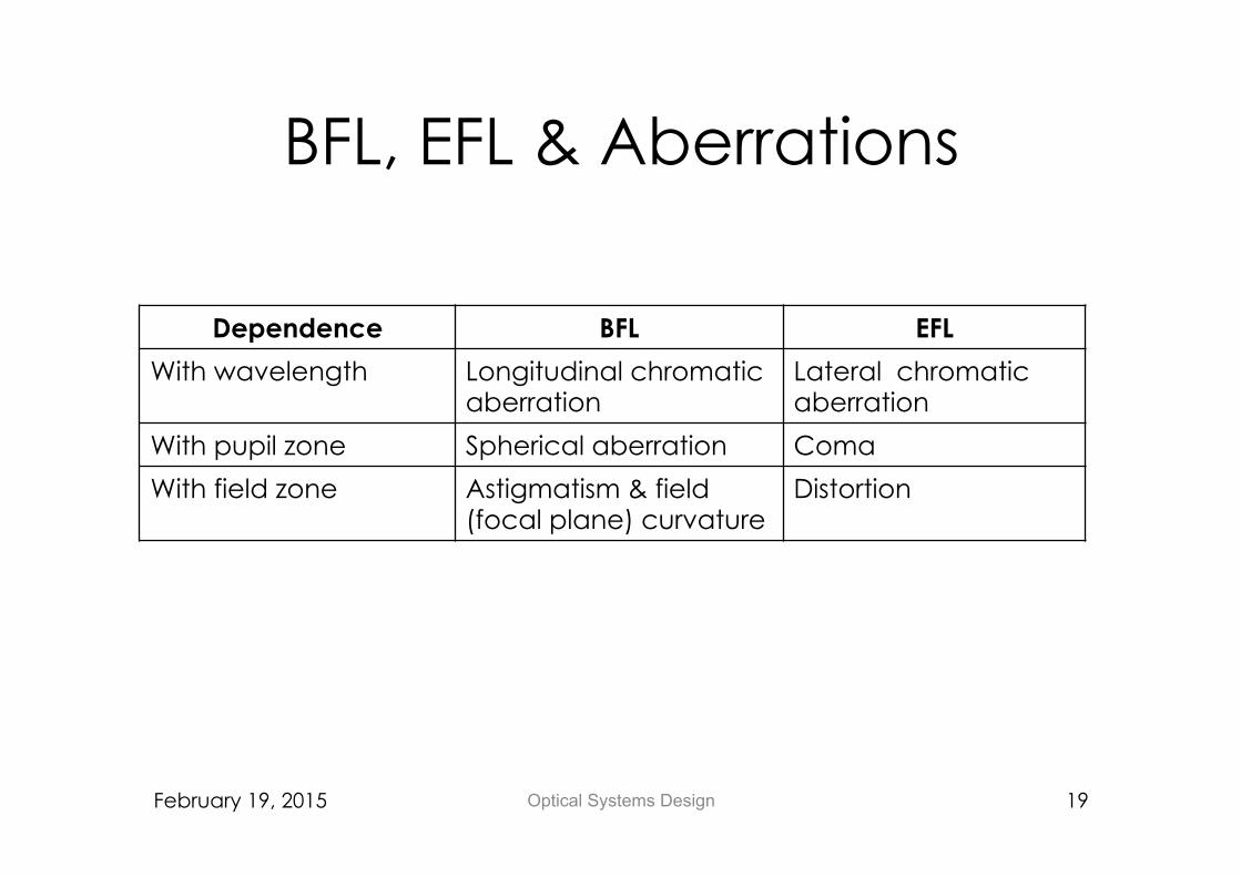
BFL, EFL & Aberrations

Dependence BFL EFL

With wavelength Longitudinal chromatic aberration

Lateral chromatic aberration

With pupil zone Spherical aberration Coma

With field zone Astigmatism & field (focal plane) curvature

Distortion

February 19, 2015 Optical Systems Design 19

Basic Zemax Analysis Tools

•  Layout plots (cross-section/shaded) •  Spot diagrams •  Ray-aberration plot

•  Optical path plot (OPD) •  Field curvature & distortion plot •  Point Spread Function (diffraction PSF) •  Modulation transfer funtion (MTF) •  Enclosed energy plot

February 19, 2015 Optical Systems Design 20

I: Layout

•  Good for basic check of obvious mistakes (e.g. data entry sign errors)

•  Sanity check after optimisation e.g. excessive surface curvatures, inappropriate glass/air thicknesses, negative edge thicknesses etc

•  Check on mechanical vignetting

February 19, 2015 Optical Systems Design 21

I: Layout

February 19, 2015 Optical Systems Design 22

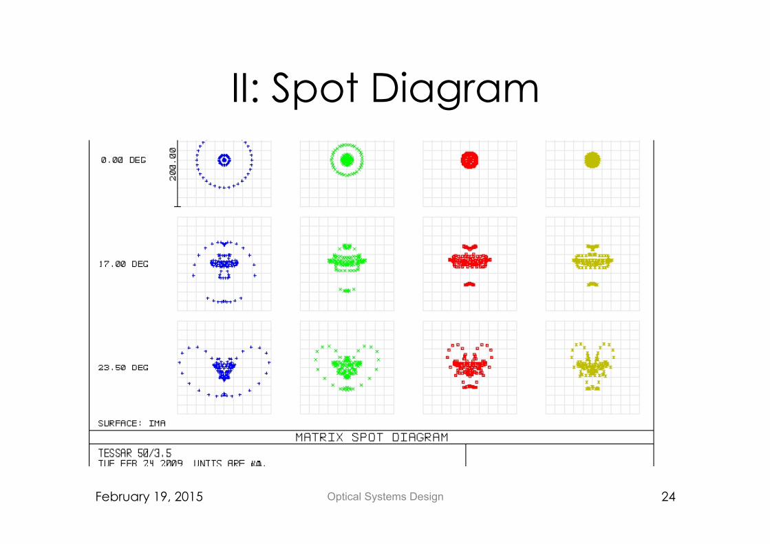
II: Spot Diagram

•  Analog of the geometrical PSF •  Shows the intersection points where a

ray bundle which fills the entrance aperture meets the image plane

•  For polychromatic (white light) systems these must be generated at representative wavelengths

February 19, 2015 Optical Systems Design 23

II: Spot Diagram

February 19, 2015 Optical Systems Design 24

III: Ray Aberration Plots

•  Spot diagrams give little information about which parts of the entrance pupil particular rays pass through

•  A given ray passes through the entrance pupil at a particular height P (-1<P<+1) and intercepts the image plane at a separation Δh from the chief ray

•  Ray aberration plots (ray fan plots) present the transverse ray height errors Δh as a function of pupil zone height P

•  Customary to present these separately for the tangential (meridional) fan and the sagittal fan

February 19, 2015 Optical Systems Design 25

III: Ray Fan Plots

February 19, 2015 Optical Systems Design 26

III: Ray Fan Plots

•  Slope of ray fan plot reflects whether image plane is close to focus (inside focus → positive slope and vice versa)

•  If effective refractive surface is curved or image surface is curved then ray fan plot also curved

•  Behavior close to origin reflects whether image plane is close to the paraxial focus

•  Each Seidel aberration has a characteristic appearance in the ray fan plot

February 19, 2015 Optical Systems Design 27

III: Ray Fan Plots

February 19, 2015 Optical Systems Design 28

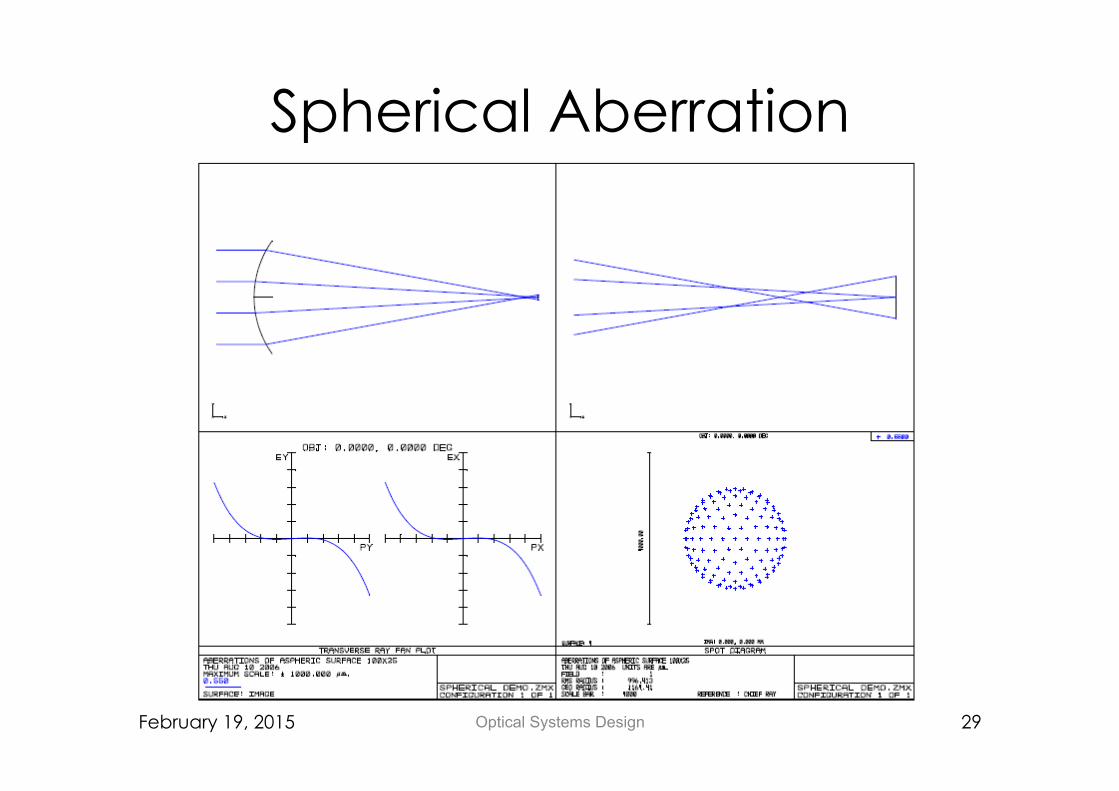
Spherical Aberration

February 19, 2015 Optical Systems Design 29

Coma

February 19, 2015 Optical Systems Design 30

Astigmatism

February 19, 2015 Optical Systems Design 31

0 deg 5 deg

Field Curvature

February 19, 2015 Optical Systems Design 32

0 deg 5 deg

Distortion

February 19, 2015 Optical Systems Design 33

0 deg 5 deg

Longitudinal Colour

February 19, 2015 Optical Systems Design 34

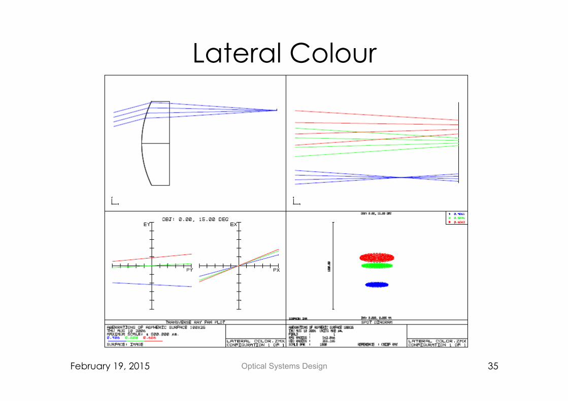
Lateral Colour

February 19, 2015 Optical Systems Design 35

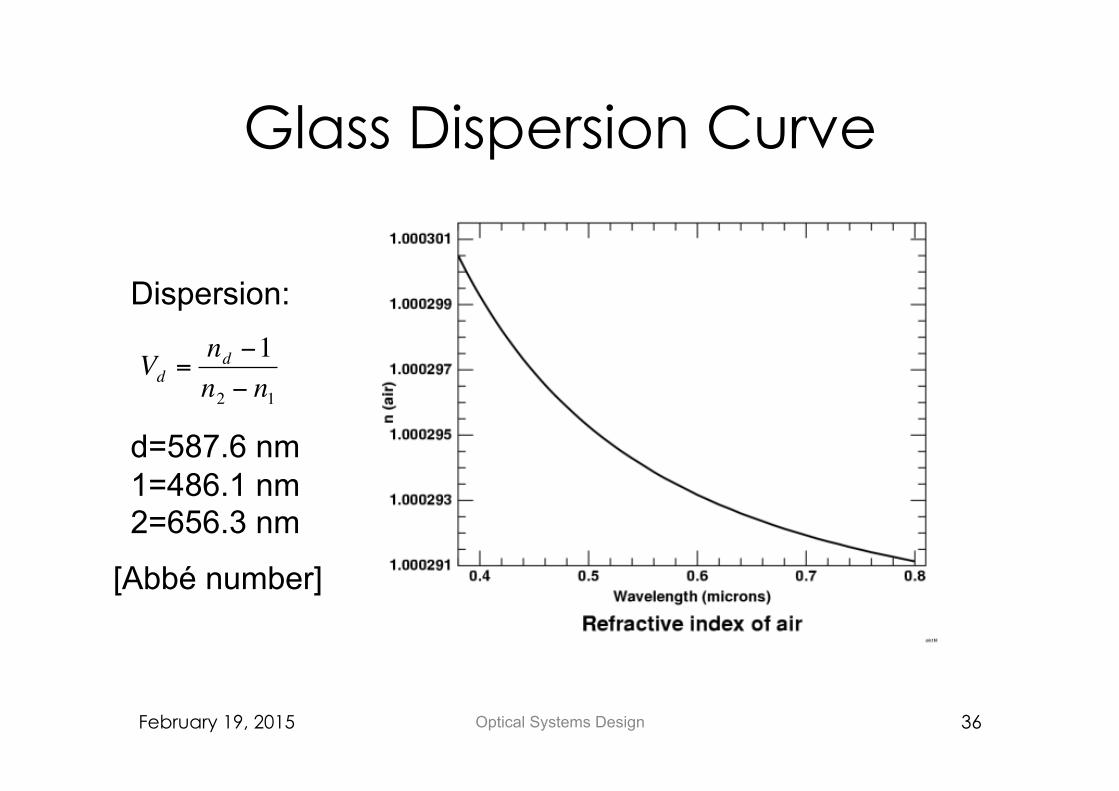
Glass Dispersion Curve

February 19, 2015 Optical Systems Design 36

Dispersion: d=587.6 nm 1=486.1 nm 2=656.3 nm

€

Vd =nd −1n2 − n1

[Abbé number]

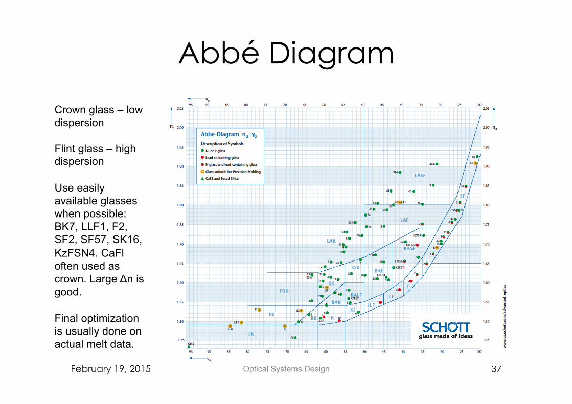
Abbé Diagram

February 19, 2015 Optical Systems Design 37

Crown glass – low dispersion Flint glass – high dispersion Use easily available glasses when possible: BK7, LLF1, F2, SF2, SF57, SK16, KzFSN4. CaFl often used as crown. Large Δn is good. Final optimization is usually done on actual melt data.

Aspheric Surfaces •  Most optical surfaces are spherical •  By far the easiest surfaces to manufacture using

conventional polishing techniques •  General rotationally symmetric optical surface has

departure from plane (sag) given by: where h2=x2+y2 is the axial height, c=1/R is the

surface curvature at the vertex, and k the conic constant. A,B,C,D are 4th, 6th, 8th, 10th order coeffs.

February 19, 2015 Optical Systems Design 38

z = ch2

1+[1−[(1+ k)c2h2 ]1/2+ Ah4 +Bh6 +Ch8 +Dh10

k=0 -1<k<0 k=-1 k<-1 k>0

sphere prolate paraboloid hyperboloid oblate

Cassegrain Telescope •  Start with a 30cm diameter F/2 spherical

primary (RoC=120cm) and a spherical secondary. Adjust the radius of curvature of the secondary to put the focus in the plane of the primary

•  Glass Type = MIRROR for reflecting surfaces; distances change sign after each reflection

•  Use a Quick-focus or M-solve to locate paraxial focus and single variables in any optimization

•  Now make primary a parabola (K=-1) •  Adjust conic constant on secondary to get best

on-axis performance

February 19, 2015 Optical Systems Design 39

Summary: Lecture 2 •  Sequential ray tracing is the main mode of Zemax

for the design of optical systems. •  Zemax has a range of optimising tools to improve

the performance of the basic design. •  The major tools for assessing performance are the

layout plots, the spot diagrams and the ray fan plots.

•  All the main Seidel aberrations have characteristic forms in these plots which can be used to decide how to improve the design.

•  Careful choice of glasses is required to remove longitudinal and lateral colour effects.

February 19, 2015 Optical Systems Design 40

Exercises: Lecture 2 •  Input the parameters of a 50mm diameter F/10

optimised (R1=265mm) achromatic doublet from Lecture 4 of the Optical Engineering Course (Dr Rolt). Take the lens thicknesses as 8mm (crown) and 4mm (flint). Investigate the axial colour over the wavelengths 0.486, 0.587 and 0.656 µm. Can you improve the performance ?  

•  Investigate the performance of the Cassegrain telescope for off-axis (1 deg) field points. What is the main off-axis aberration ?  

•  Try to minimize this aberration by making both the primary and secondary hyperbolic.

February 19, 2015 Optical Systems Design 41