Lecture 19: Uncertainty 4 Victor R. Lesser

Lecture 19: Uncertainty 4

Victor R. Lesser CMPSCI 683

Fall 2010

V. Lesser; CS683, F10

Today’s Lecture

  Inference in Multiply Connected BNs   Clustering methods transform the network into a probabilistically

equivalent polytree.   Also called Join tree algorithms

  Conditioning methods instantiate certain variables and evaluate a polytree for each possible instantiation.

  Stochastic simulation approximate the beliefs by generating a large number of concrete models that are consistent with the evidence and CPTs.


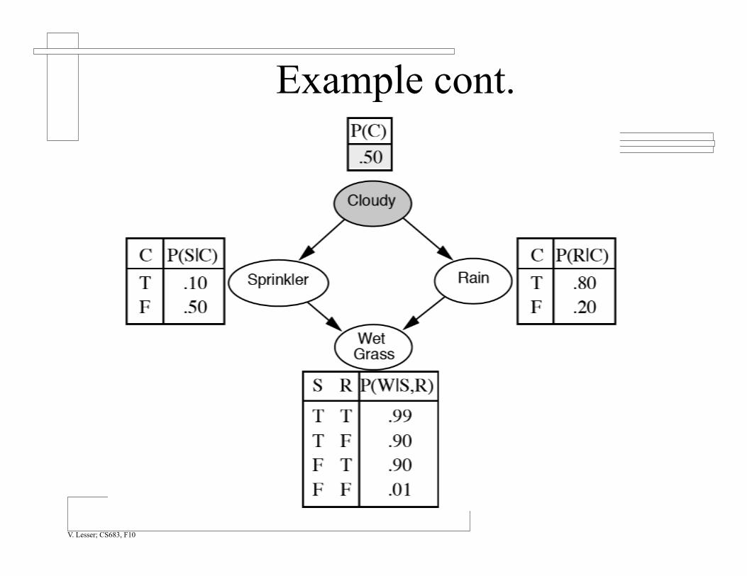
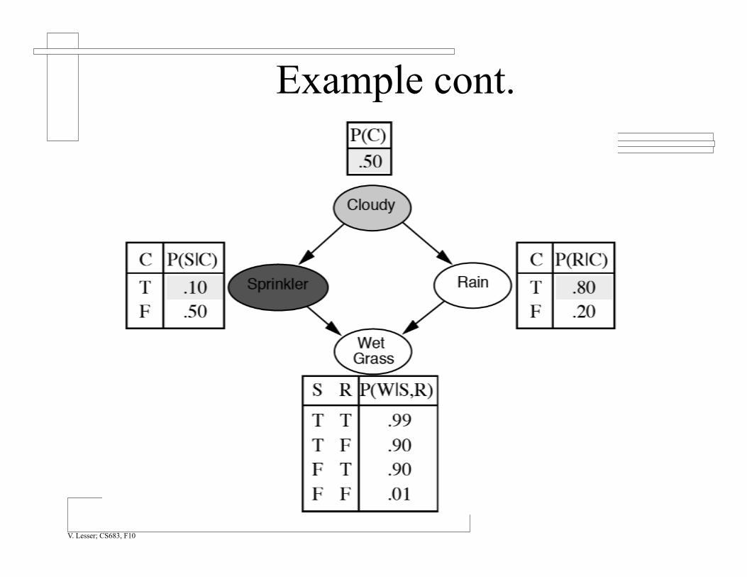
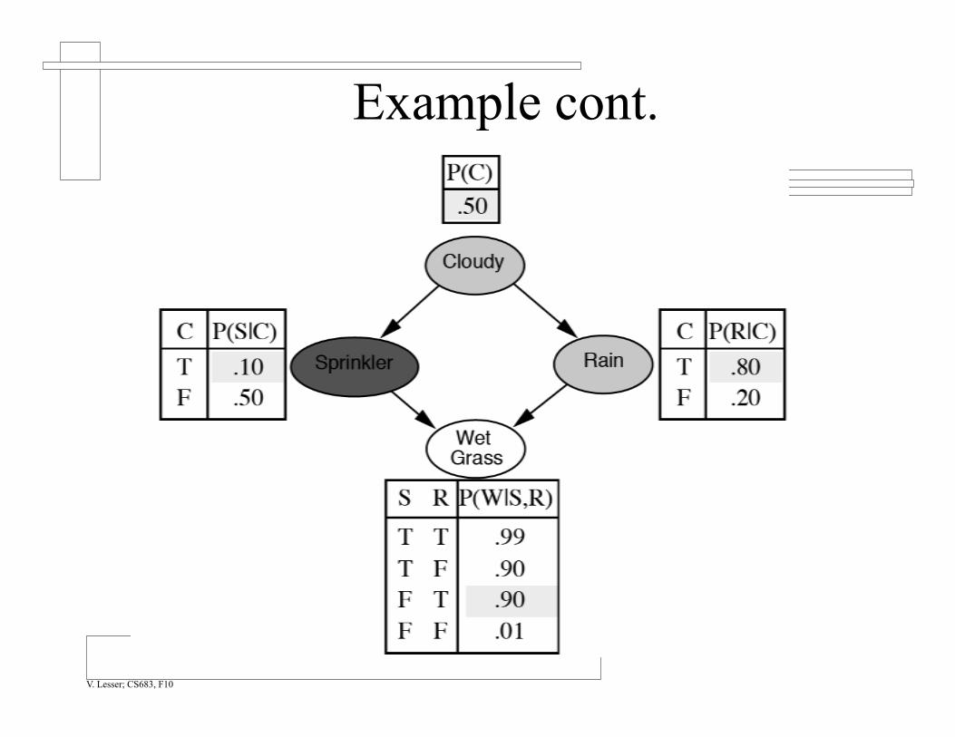
Example of Multiply Connected BN

Cloudy

Sprinkler Rain

Wet Grass

C P(S=T) T .10 F .50

C P(R=T) T .80 F .20

P(C=T)=.5

S R P(W=T) T T .99 T F .90 F T .90 F F .00


Clustering Methods

 Creating meganodes until the network becomes a polytree.

 Most effective approach for exact evaluation of multiply connected BNs.

 The tricky part is choosing the right meganodes.

 Q. What happens to the NP-hardness of the inference problem?


Clustering Example*

Cloudy

Spr+Rain

Wet Grass

P(S+R) C TT TF FT FF T .08 .02 .72 .18 F .10 .40 .10 .40

P(C)=.5

S+R P(W) T T .99 T F .90 F T .90 F F .00

Cloudy

Sprinkler Rain

Wet Grass

How do you still answer P(Rain=True | Wet Grass=False) ? How do you create meganode? What are the disadvantages?


Cutset Conditioning Methods

 Once a variable is instantiated it can be duplicated and thus “break” a cycle.

 A cutset is a set of variables whose instantiation makes the graph a polytree.

 Each polytree’s likelihood is used as a weight when combining the results.


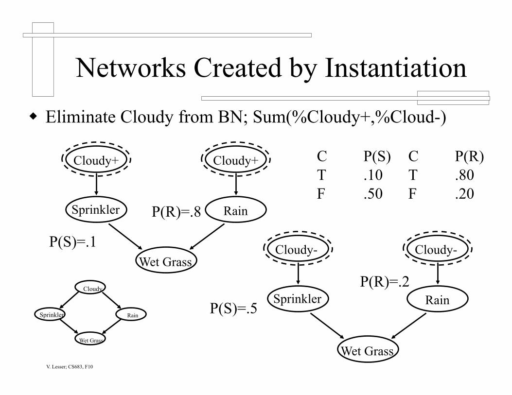
Networks Created by Instantiation   Eliminate Cloudy from BN; Sum(%Cloudy+,%Cloud-)

C P(R) T .80 F .20

Cloudy+

Sprinkler Rain

Wet Grass

Cloudy+

Cloudy-

Sprinkler Rain

Wet Grass

Cloudy-

C P(S) T .10 F .50

P(S)=.1

P(S)=.5

P(R)=.8

P(R)=.2 Cloudy

Sprinkler Rain

Wet Grass


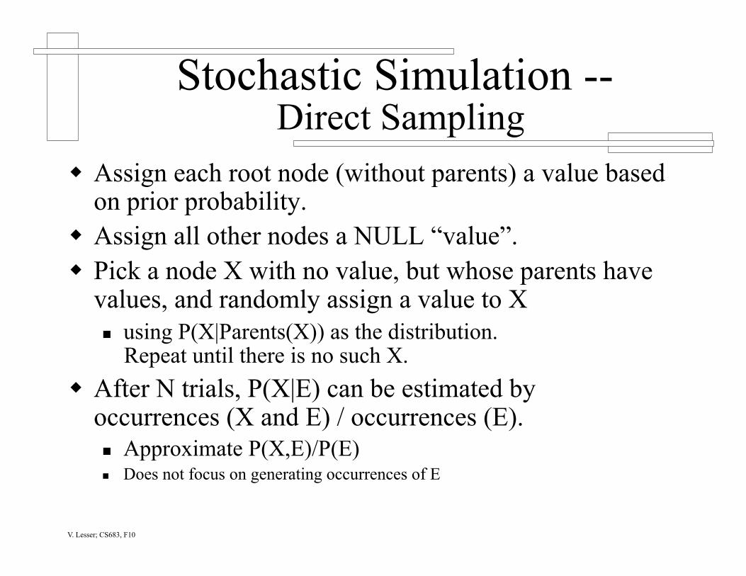
Stochastic Simulation -- Direct Sampling

  Assign each root node (without parents) a value based on prior probability.

  Assign all other nodes a NULL “value”.   Pick a node X with no value, but whose parents have

values, and randomly assign a value to X   using P(X|Parents(X)) as the distribution.

Repeat until there is no such X.   After N trials, P(X|E) can be estimated by

occurrences (X and E) / occurrences (E).   Approximate P(X,E)/P(E)   Does not focus on generating occurrences of E

Example P(WetGrass|Cloudy)


Example cont.


Example cont.


Example cont.


Example cont.


Example cont.


Example cont.



Stochastic Simulation cont.

 Problem with very unlikely events.  Likelihood weighting can be used to

fix problem.  Likelihood weighting converges

much faster than logic sampling and works well for very large networks.


Example of Likelihood Weighting P(WetGrass | Rain)

  Choose a value for Cloudy with prior P(Cloudy) = 0.5. Assume we choose cloudy = false.

  Choose a value for Sprinkler. We see that P(Sprinkler ⏐¬ Cloudy) = 0.5, so we randomly choose a value given that distribution. Assume we choose Sprinkler =True.

  Look at Rain. This is an evidence variable that has been set to True, so we look at the table to see that P(Rain ⏐¬ Cloudy) = 0.2. This run therefore counts as 0.2 of a complete run.

Cloudy

Sprinkler Rain

Wet Grass


Example of Likelihood Weighty cont’d

  Look at WetGrass. Choose randomly with P(WetGrass⏐Sprinkler=T ∧Rain=T) =0.99; assume we choose WetGrass = True.

  We now have completed a run with likelihood 0.2 that says WetGrass = True given Rain = True. The next run will result in a different likelihood, and (possibly) a different value for WetGrass. We continue until we have accumulated enough runs, and then add up the evidence for each value, weighted by the likelihood score.

Likelihood weighting usually converges much faster than logic sampling

Still takes a long time to reach accurate probabilities for unlikely events

Stochastic Simulation – Likelihood Weighting


; for all nodes in the network ordered by parents

; if you are at the node that you have evidence for ; adjust likelihood of this run based on the likelihood of evidence given parents

;otherwise randomly choose based on value of parents chosen in previous steps

Likelihood weighting example

w = 1.0

P(Rain| Sprinkler=T, WetGrass=T)


Example cont.

w = 1.0


Example cont.

w = 1.0 × 0.1


Example cont.

w = 1.0 × 0.1


Example cont.

W = 1.0 × 0.1 × 0.99 = 0.099



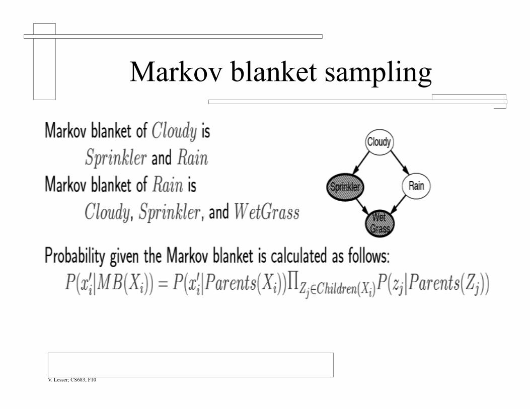
Stochastic Simulation – Markov Chain Monte Carlo

A node is conditionally independent of all other nodes in the network given its parents, children, and children’s parents—that is, given its Markov blanket.


The MCMC algorithm

  MCMC generates each event by making a random change to the preceding event.   It is therefore helpful to think of the network being in a

particular current state specifying a value for every variable.

  The next state is generated by randomly sampling a value for one of the non-evidence variables Xi, conditioned on the current values of the variables in the Markov blanket of Xi.   Don’t need to look at any other variables

  MCMC therefore wanders randomly around the state space—the space of possible complete assignments—flipping one variable at a time but keeping the evidence variables fixed.


The Markov chain


Markov blanket sampling


MCMC example cont.


Summary of a Belief Networks   Conditional independence information is a vital and

robust way to structure information about an uncertain domain.

  Belief networks are a natural way to represent conditional independence information.   The links between nodes represent the qualitative aspects of the

domain, and the conditional probability tables represent the quantitative aspects.

  A belief network is a complete representation for the joint probability distribution for the domain, but is often exponentially smaller in size.


Summary of a Belief Networks, cont’d

  Inference in belief networks means computing the probability distribution of a set of query variables, given a set of evidence variables.

  Belief networks can reason causally, diagnostically, in mixed mode, or intercausally. No other uncertain reasoning mechanism can handle all these modes.

  The complexity of belief network inference depends on the network structure. In polytrees (singly connected networks), the computation time is linear in the size of the network.


Summary of a Belief Networks, cont’d   There are various inference techniques for general belief

networks, all of which have exponential complexity in the worst case.   In real domains, the local structure tends to make things more

feasible, but care is needed to construct a tractable network with more than a hundred nodes.

  It is also possible to use approximation techniques, including stochastic simulation, to get an estimate of the true probabilities with less computation.

Next Lecture

 Introduction to Decision Theory

  Making Single-Shot Decisions

  Utility Theory


Lecture 19: Uncertainty 4 Victor R. Lesser

Documents