1 Lecture 18: One and two locus models of selection Bruce Walsh lecture notes Synbreed course version 8 July 2013

Welcome message from author
This document is posted to help you gain knowledge. Please leave a comment to let me know what you think about it! Share it to your friends and learn new things together.
Transcript

1
Lecture 18:
One and two locus models of
selection
Bruce Walsh lecture notes
Synbreed course
version 8 July 2013
2
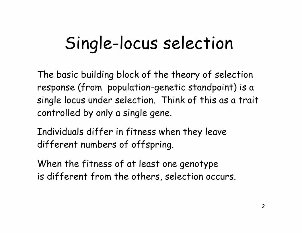
Single-locus selection
The basic building block of the theory of selection
response (from population-genetic standpoint) is a
single locus under selection. Think of this as a trait
controlled by only a single gene.
Individuals differ in fitness when they leave
different numbers of offspring.
When the fitness of at least one genotype
is different from the others, selection occurs.
3
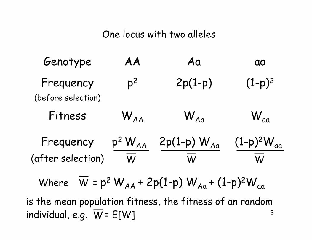
(1-p)2Waa2p(1-p) WAap2 WAAFrequency
(after selection)
WaaWAaWAAFitness
(1-p)22p(1-p)p2Frequency(before selection)
aaAaAAGenotype
One locus with two alleles
W W W
W
is the mean population fitness, the fitness of an random
individual, e.g. = E[W]
Where = p2 WAA + 2p(1-p) WAa + (1-p)2WaaW
4
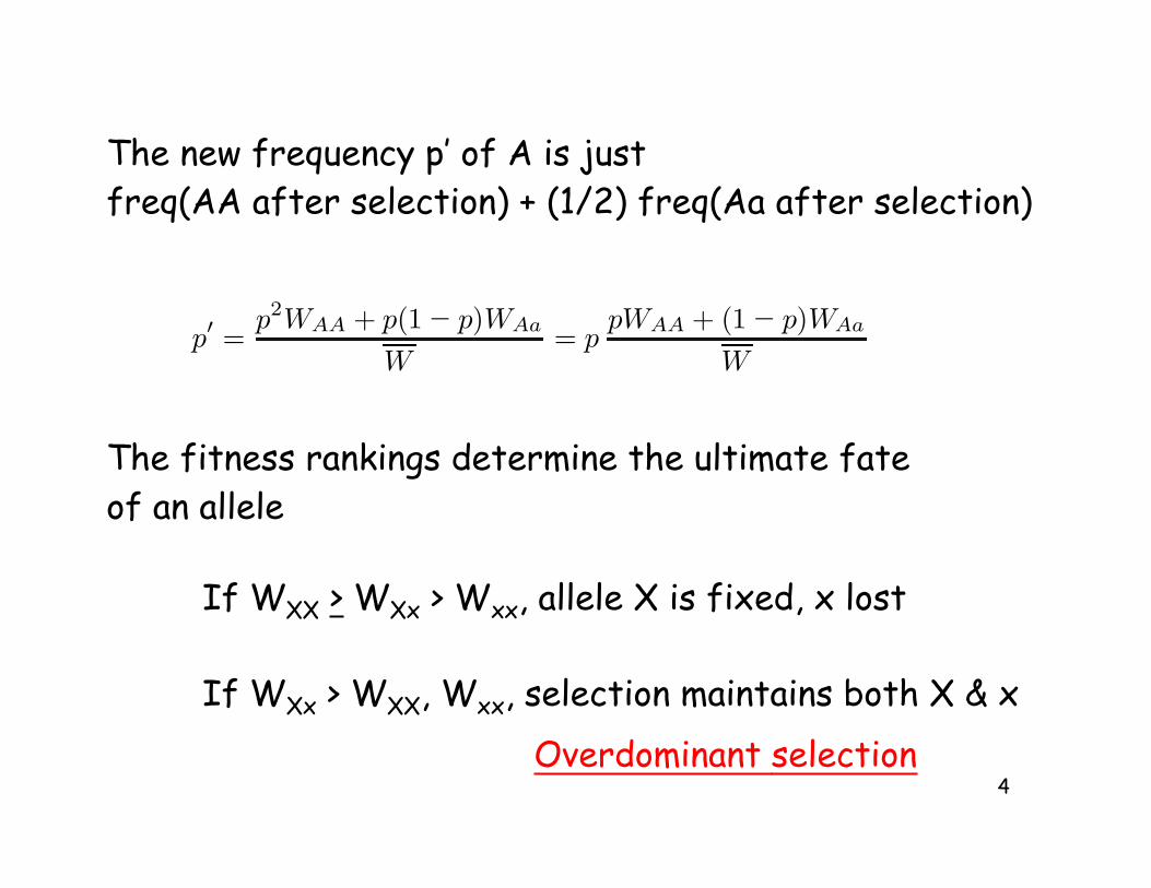
The new frequency p’ of A is just
freq(AA after selection) + (1/2) freq(Aa after selection)
p′ =p2WAA + p(1− p)WAa
W= p
pWAA + (1− p)WAa
W
The fitness rankings determine the ultimate fate
of an allele
If WXX > WXx > Wxx, allele X is fixed, x lost
If WXx > WXX, Wxx, selection maintains both X & x
Overdominant selection

5

6
Class problem: Required time for allele
frequency change
Compute the time to change from frequency 0.1 to 0.9
(i) Fitness are 1 : 1.01: 1.02
(ii) Fitness are 1: 1:02: 1.02
(iii) Fitness are 1: 1: 1.02
7
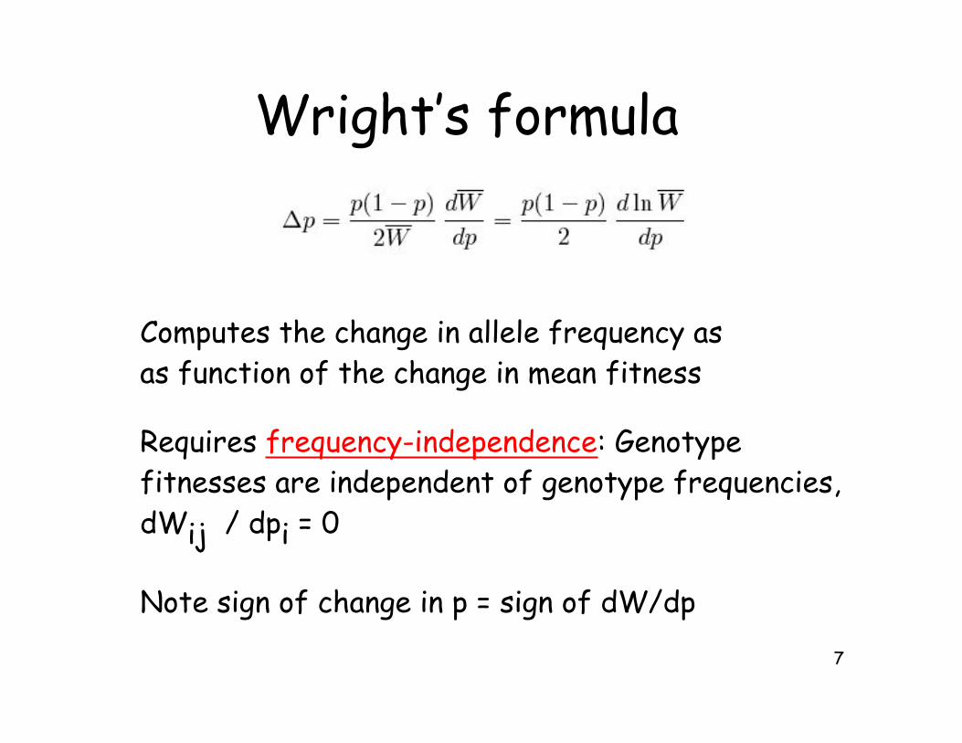
Wright’s formula
Computes the change in allele frequency as
as function of the change in mean fitness
Requires frequency-independence: Genotype
fitnesses are independent of genotype frequencies,
dWij / dpi = 0
Note sign of change in p = sign of dW/dp

8
Application: Overdominant selection
Key: Internal equilibrium frequency.
Stable equilibrium

9
Application: Stabilizing selection
This is selective underdominance! If p < 1/2, !p < 0
and allele gets lost. If p > 1/2, !p > 0 and allele
fixed.
Hence, stabilizing selection on a trait controlled by
many loci removes variation!
A common model for stabilizing selection
on a trait is to use a normal-type
curve for trait fitness
As detailed in WL Example 5.6, we can use Wright’s formula
to compute allele frequency change under this type of
selection

10
p′i = pi
Wi
W, Wi =
n∑
j=1
pjWij , W =n∑
i=1
piWi
Multiple Alleles
Let pi = freq(Ai), Wij = fitness AiAj
Wi = marginal fitness of allele Ai
W = mean population fitness = E[Wi] = E[Wij]
If Wi > W, allele Ai increases in frequency
If a selective equilibrium exists, then Wi = W
for all segregating alleles.
11
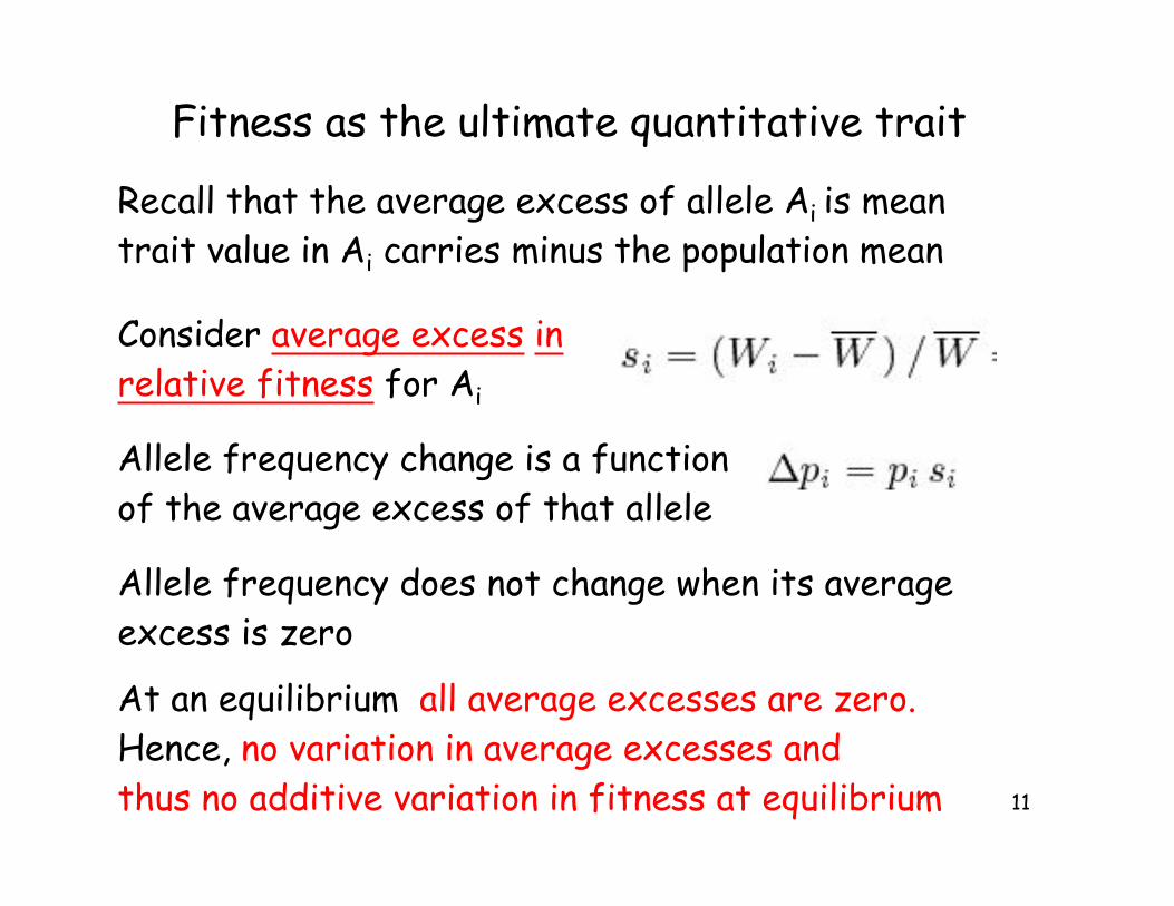
Fitness as the ultimate quantitative trait
Recall that the average excess of allele Ai is mean
trait value in Ai carries minus the population mean
Consider average excess in
relative fitness for Ai
Allele frequency change is a function
of the average excess of that allele
Allele frequency does not change when its average
excess is zero
At an equilibrium, all average excesses are zero.
Hence, no variation in average excesses and
thus no additive variation in fitness at equilibrium

12
Wright’s formula with multiple alleles
Key: Note that the sign of dW/dpi does not determine
sign(!p). Thus an allele can change in a direction
opposite to that favored by selection if the changes
on the other alleles improve fitness to a greater extent
Prelude to the multivariate breeder’s equation, R = G"

13
General features with multiple
allele selection
With Wij constant and random mating, mean fitness
always increases
What about polymorphic equilibrium?
Require Wi = W1 for all i.
Kingman showed there are only either zero, one, or
infinitely many sets of equilibrium frequencies for
an internal equilibrium (all alleles are segregating).
14
p1
p3p2
1
11
p1 + p2 + p3 = 1
corner
equilibrium
edge
equilibrium
internal
equilibrium
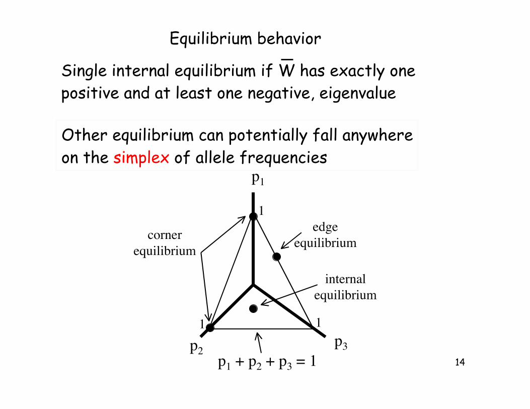
Equilibrium behavior
Other equilibrium can potentially fall anywhere
on the simplex of allele frequencies
Single internal equilibrium if W has exactly one
positive and at least one negative, eigenvalue

15
Two-locus selection
When two (or more) loci are under selection, single
locus theory no longer holds, because of linkage
disequilibrium, D = freq(ab) - freq(a)*freq(b)
Consider the marginal fitness of the AA genotype

16
Two-locus selection
Here, W(AA) is independent of freq(A) = p, and
we can use Wright’s formula to compute allele
frequency change. Can’t do this when D not zero!
Note that this is a function of p = freq(A), q=freq(B),
and D = freq(AB)-p*q. When D = 0 this reduces to
17
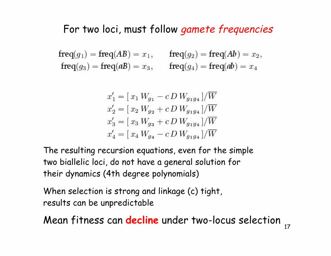
For two loci, must follow gamete frequencies
The resulting recursion equations, even for the simple
two biallelic loci, do not have a general solution for
their dynamics (4th degree polynomials)
When selection is strong and linkage (c) tight,
results can be unpredictable
Mean fitness can decline under two-locus selection

18
At equilibrium
If LD at equilibrium, the second term is nonzero and
not all gametes have the same marginal fitness. Note
that when c = 0, this is just a 4 allele model, and all
segregating alleles have the same marginal fitness
If equilibrium LD is not zero, mean fitness is not
at a local maximum. However, unless c is very small,
it is usually close
In such cases, mean fitness decreases during the final approach
to the equilibrium (again, effects usually small)

19
Note complete additivity in the trait.
W(z) = 1 - s(z-2)2
Fitness function induces dominance and epistasis
for a completely additive trait
At equilibrium, no additive variance in FITNESS -- still
could have lots of additive variance in the trait.
WL Example 5.11. Even apparently simple models can have
complex behavior.

20
FFT: Fisher’s Fundamental Theorem
What, in general can be said above the behavior of
multilocus systems under selection?
Other than they are complex, no general statement!
Some rough rules arise under certain generalizations,
such as weak selection -- weak selection on each
individual locus, selection on the trait could be strong.
One such rule, widely abused, is Fisher’s Fundamental
theorem
Karlin: “FFT is neither fundamental nor a theorem”

21
Fisher: “The rate of increase in fitness of any
organism at any time is equal to its genetic variance
in fitness at that time”
Classical Interpretation: ! Wbar = VarA(fitness)
This interpretation holds exactly only under restricted
conditions, but is often a good approximate descriptor
Important corollary holds under very general conditions: in
the absence of new variation from mutation or other
sources such as migration, selection is expected to
eventually remove all additive genetic variation in fitness
For example, approximately true under weak selection
22
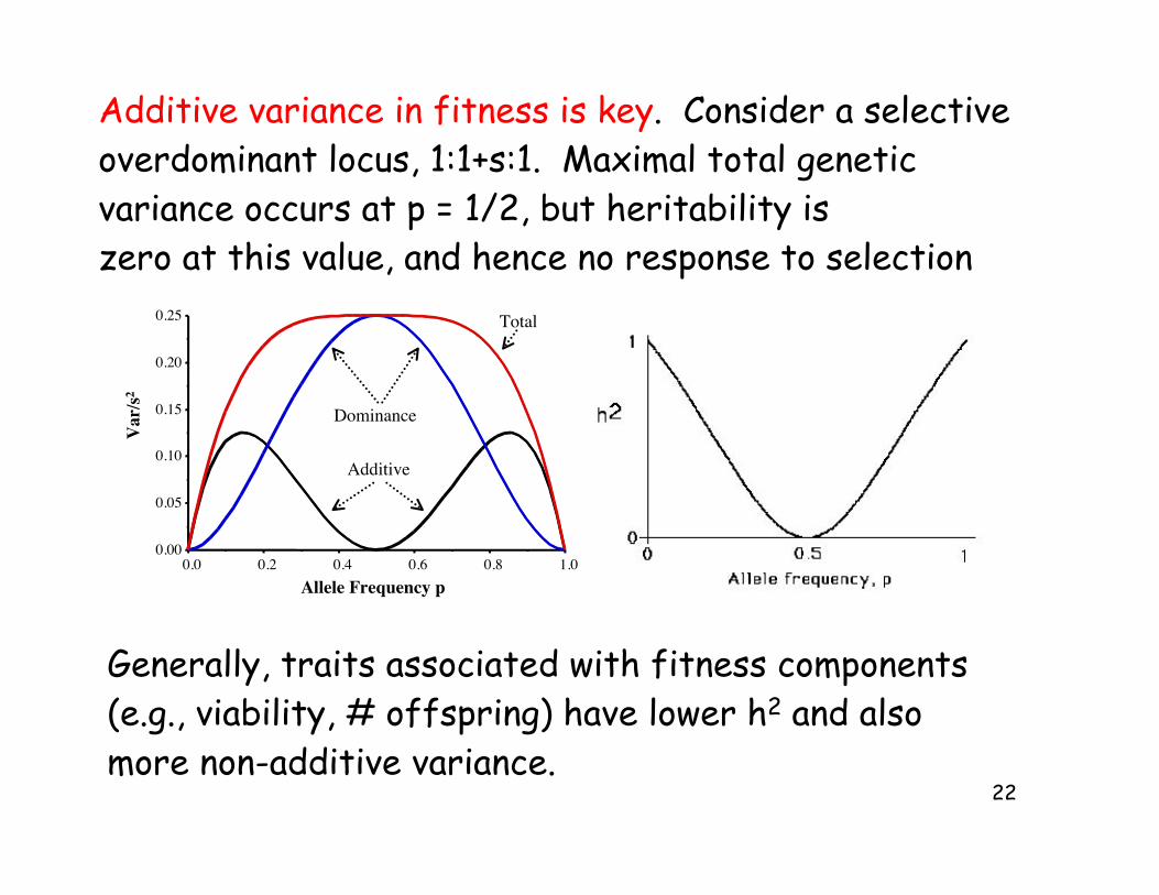
Additive variance in fitness is key. Consider a selective
overdominant locus, 1:1+s:1. Maximal total genetic
variance occurs at p = 1/2, but heritability is
zero at this value, and hence no response to selection
Generally, traits associated with fitness components
(e.g., viability, # offspring) have lower h2 and also
more non-additive variance.
1.00.80.60.40.20.0
0.00
0.05
0.10
0.15
0.20
0.25
Allele Frequency p
Var/
s2
Additive
Dominance
Total

23
0.80.70.60.50.40.30.20.10.0
.001
.01
.1
1
Heritability
Pro
po
rtio
n o
f fi
tnes
s ex
pla
ined
Traits more closely associated (phenotypically correlated) with fitness had lower
heritabilities in Collared flycatchers (Ficedula albicollis) on the island of
Gotland in the Baltic sea, (Gustafsson 1986)
24
0.50.40.30.20.10.0
0.0
0.2
0.4
0.6
0.8
1.0
Heritability
Co
rrel
ati
on
wit
h f
ruit
pro
du
ctio
n
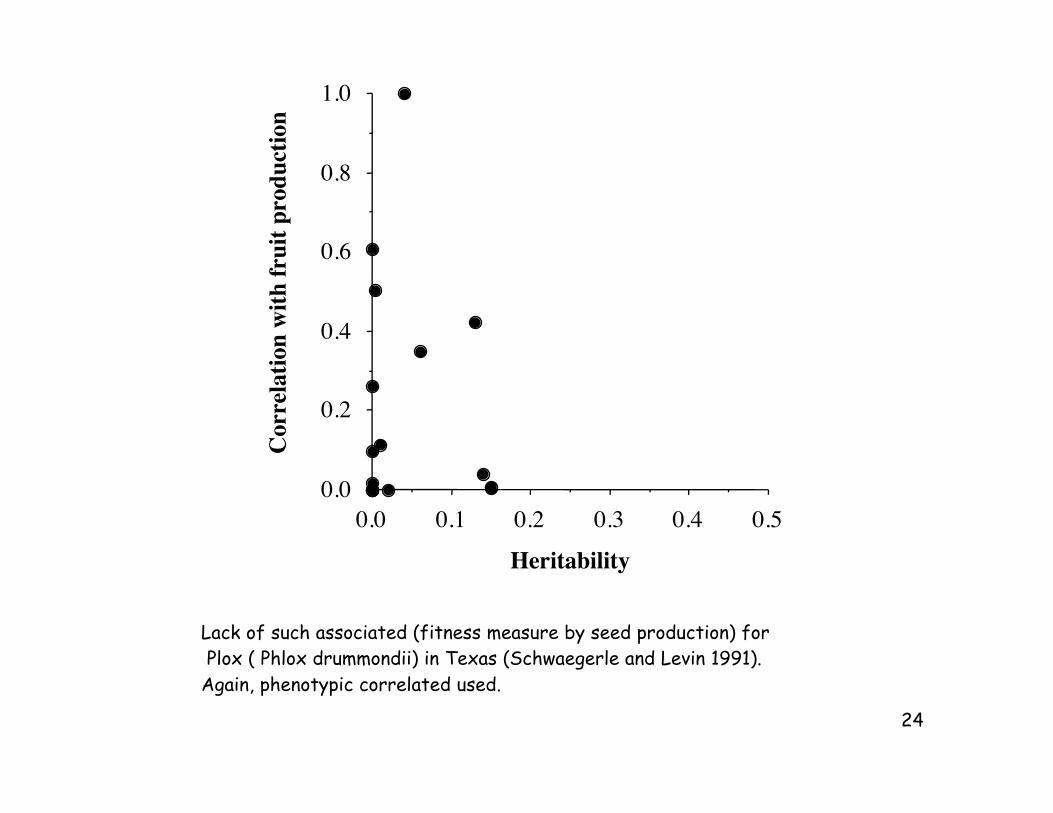
Lack of such associated (fitness measure by seed production) for
Plox ( Phlox drummondii) in Texas (Schwaegerle and Levin 1991).
Again, phenotypic correlated used.

25
Life history and morphological traits in the Scottish red deer ( Cervus elaphus).
Circles denote life-history traits, squares morphological traits. Genetic correlation
between trait and fitness (Kruuk et al. 2000)

26
Common is variance standarization, x’ = x/#x
Houle: Evolvability
Traits are generally standardized to compare them
with others:
Houle agreed that our interest is typically in the
proportion of change -- e.g, animals are 5% larger.
With variance-standardization, a response of 0.1 implies
a 0.1 standard-deviation change in the mean.
Variance-standardization thus a function of standing
variation in the population.
Evolvability uses mean standardization, x’ = x/µ
A 0.1 response on this scale means the trait improved by
10%

27
Houle: Evolvability
Houle argued that evolvability of a trait, CVA = #A/ µ
(mean-standardization) is a better measure of evolutionary
potential than h2 = #A2 / #z
2 (variance-standardization)
Houle found that life history traits had HIGHER
evolvabilities = significant potential for large
proportional (percentage) change in the mean
They had more genetic variation, but also
more environmental variance, resulting in lower h2
28
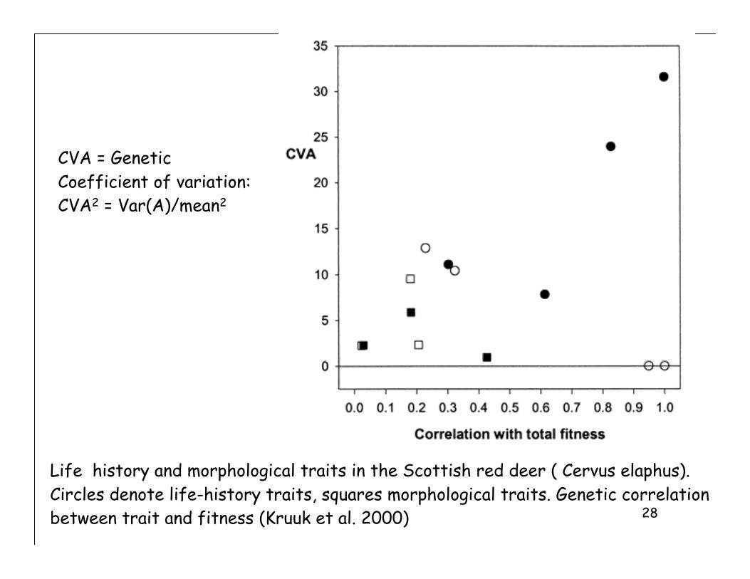
Life history and morphological traits in the Scottish red deer ( Cervus elaphus).
Circles denote life-history traits, squares morphological traits. Genetic correlation
between trait and fitness (Kruuk et al. 2000)
CVA = Genetic
Coefficient of variation:
CVA2 = Var(A)/mean2

29
How much selection on a QTL given selection
on a trait?
Having a specific
allele shifts the
overall trait
distribution slightly
Resulting strength (and
form) of selection on a
QTL
30
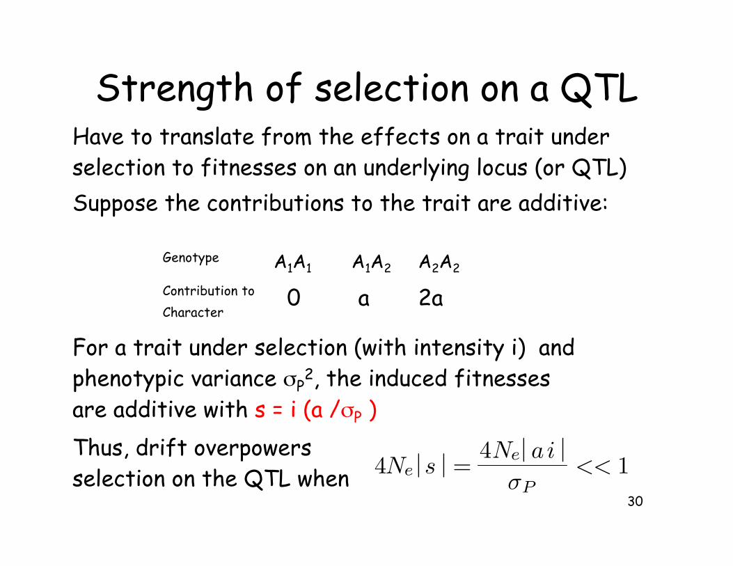
Strength of selection on a QTL
2a a 0Contribution to
Character
A2A2A1A2A1A1Genotype
Have to translate from the effects on a trait under
selection to fitnesses on an underlying locus (or QTL)
Suppose the contributions to the trait are additive:
For a trait under selection (with intensity i) and
phenotypic variance #P2, the induced fitnesses
are additive with s = i (a /#P )
Thus, drift overpowers
selection on the QTL when4Ne |s | =
4Ne| ai |σP
<< 1

31
More generally
1+2s1+s(1+h)1Fitness
2aa(1+k)0Contribution to trait
A2A2A1A2A1A1Genotype
∆q " 2q(1 q)[1 + h(1 − 2q)]Change in allele frequency:
s = i (a /#P )
Selection coefficients for a QTL
h = k

32
Class problem: How quickly do allele
frequencies at a QTL change?
2a a 0Contribution to
Character
A2A2A1A2A1A1Genotype
s = i (a /#P )
(1) Suppose a/# = 0.5
Suppose i = 2 (strong TRAIT selection). How
long for a rare QTL (p0 = 0.05) to reach 50%?
(2) Suppose a/# = 0.005

33
General selection response• Two locus theory in the general setting is
very complex!
• What can we say about k-locus selection?
• FFT under weak selection gives someapproximate rules about how populationsevolve by following changes in fitness
• We are usually much more interested inchanges in trait values. What can we sayhere?
• Robertson’s secondary theorem

34
Robertson’s secondary theorem and the
breeder’s equation
Alan Robertson proposed a “secondary theorem”
to Fisher’s to treat trait evolution,
Response = change in mean equals the additive
genetic covariance between trait and fitness
(the covariance within an individual for the
breeding values of these two traits).

35
Much more on FFT, Robertson’s theorem, set within
the Price-equation framework (no covered here) in WL
Chapter 6
36
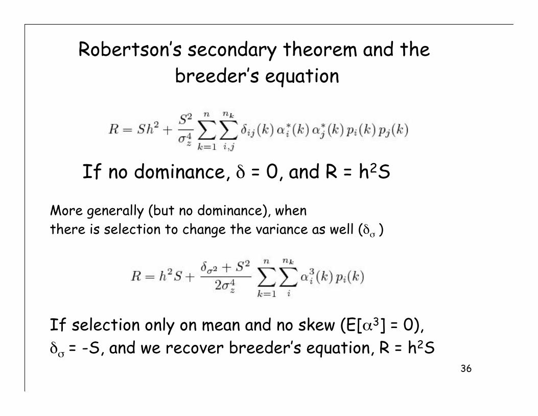
Robertson’s secondary theorem and the
breeder’s equation
If no dominance, $ = 0, and R = h2S
More generally (but no dominance), when
there is selection to change the variance as well ($# )
If selection only on mean and no skew (E[%3] = 0),
$# = -S, and we recover breeder’s equation, R = h2S
Related Documents