Lecture 17 -- Beam Propagation Methodemlab.utep.edu/ee5390cem/Lecture 17 -- Beam Propagation Method.pdf · Beam Propagation Method These notes may contain copyrighted material obtained

7/21/2017

1

Lecture 17 Slide 1

EE 5337

Computational Electromagnetics (CEM)

Lecture #17

Beam Propagation Method These notes may contain copyrighted material obtained under fair use rules.  Distribution of these materials is strictly prohibited  

InstructorDr. Raymond Rumpf(915) 747‐[email protected]

Outline

• Overview

• Formulation of 2D finite‐difference beam propagation method (FD‐BPM)

• Implementation of 2D FD‐BPM

• Formulation of 3D FD‐BPM

• Alternative formulations of BPM

– FFT‐BPM

– Wide Angle FD‐BPM

– Bi‐Directional BPM

Lecture 17 Slide 2

7/21/2017

2

Lecture 17 Slide 3

Overview

Lecture 17 Slide 4

Geometry of BPM

z

x

longitudinal direction

tran

sverse direction

BPM is primarily a “forward” propagating algorithm where the dominant direction of propagation is longitudinal.

The grid is computed and interpreted as it is in FDFD.   The algorithm and implementation looks more like the method of lines than it does FDFD.

BPM is implemented on a grid.  There are no layers.

7/21/2017

3

Lecture 17 Slide 5

Example Simulation of a Coupled‐Line Filter

This animation is NOT of the wave propagating through the device.  Instead, it is the sequence of how the solution is calculated.

Lecture 17 Slide 6

Formulation of 2D Finite‐Difference 

Beam Propagation Method

7/21/2017

4

Lecture 17 Slide 7

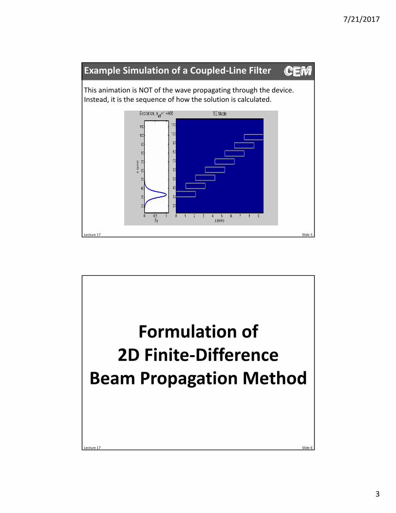
Starting Point

We start with Maxwell’s equations in the following form.

yzxx x

x zyy y

y xzz z

EEH

y z

E EH

z xE E

Hx y

yzxx x

x zyy y

y xzz z

HHE

y z

H HE

z x

H HE

x y

Recall that we have normalized the grid according to

0x k x 0y k y 0z k z

Recall that the material properties potentially incorporate a PML at the x and y axis boundaries (propagation along z).

y xxx xx yy yy zz zz x y

x y

s ss s

s s

y xxx xx yy yy zz zz x y

x y

s ss s

s s

Lecture 17 Slide 8

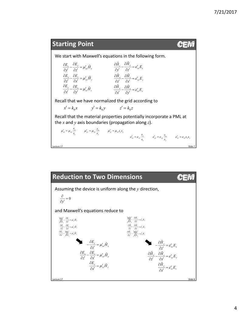
Reduction to Two Dimensions

Assuming the device is uniform along the y direction, 

zE

y

yxx x

x zyy y

y x

EH

z

E EH

z xE E

x y

zz zH

zH

y

y

xx x

x zyy y

y x

HE

z

H HE

z x

H H

x y

zz zE

0y

and Maxwell’s equations reduce to

yxx x

x zyy y

yzz z

EH

zE E

Hz x

EH

x

yxx x

x zyy y

yzz z

HE

z

H HE

z x

HE

x

7/21/2017

5

Lecture 17 Slide 9

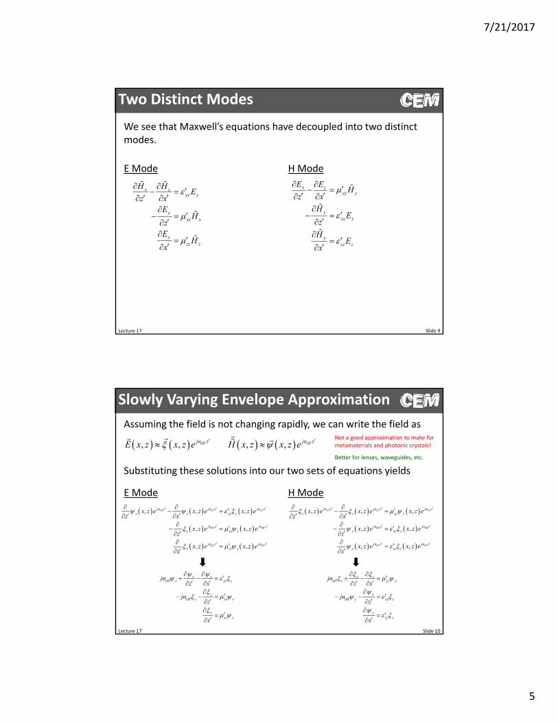
Two Distinct Modes

We see that Maxwell’s equations have decoupled into two distinct modes.

E Mode

x zyy y

yxx x

yzz z

H HE

z xE

HzE

Hx

H Mode

x zyy y

yxx x

yzz z

E EH

z x

HE

z

HE

x

Lecture 17 Slide 10

Slowly Varying Envelope Approximation

Assuming the field is not changing rapidly, we can write the field as

eff eff, , , ,jn z jn zE x z x z e H x z x z e

Substituting these solutions into our two sets of equations yields

E Mode

eff eff eff

eff eff

eff eff

, , ,

, ,

, ,

jn z jn z jn zx z yy y

jn z jn zy xx x

jn z jn zy zz z

x z e x z e x z ez x

x z e x z ez

x z e x z ex

H Mode

eff eff eff

eff eff

eff eff

, , ,

, ,

, ,

jn z jn z jn zx z yy y

jn z jn zy xx x

jn z jn zy zz z

x z e x z e x z ez x

x z e x z ez

x z e x z ex

eff

eff

x zx yy y

yy xx x

yzz z

jnz x

jnz

x

eff

eff

x zx yy y

yy xx x

yzz z

jnz x

jnz

x

Not a good approximation to make for metamaterials and photonic crystals!

Better for lenses, waveguides, etc.

7/21/2017

6

Lecture 17 Slide 11

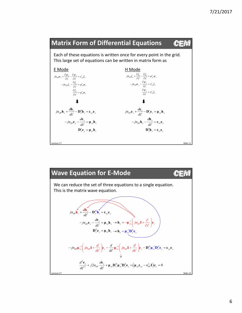
Matrix Form of Differential Equations

Each of these equations is written once for every point in the grid.  This large set of equations can be written in matrix form as

E Mode H Mode

eff

eff

x zx yy y

yy xx x

yzz z

jnz x

jnz

x

eff

eff

hxx x z yy y

yy xx x

ex y zz z

djn

dzd

jndz

hh D h ε e

ee μ h

D e μ h

eff

eff

x zx yy y

yy xx x

yzz z

jnz x

jnz

x

eff

eff

exx x z yy y

yy xx x

hx y zz z

djn

dzd

jndz

ee D e μ h

hh ε e

D h ε e

Lecture 17 Slide 12

Wave Equation for E‐Mode

We can reduce the set of three equations to a single equation.  This is the matrix wave equation.

eff

eff

Hx yy y

yy xx x

Ex y zz

xz

z

x

djn

dzd

jndz

D ε e

ee μ h

D e μ

h h

h

h

eff

21 2

eff eff2

11 1eff eff

2 0

H Ezz xx yy y

y y H Exx x zz x y xx

yxx y xx y

yy y

djn

dz

d dj n n

d djn jn

dz d

dz d

z

z

μ DD εe e

e eμ D μ D e μ ε I

μ I e

e

μ I e

1

1effxx

zz x

y

Ez

x

y

jnz

μ D

μ I

h

e

e

h

7/21/2017

7

Lecture 17 Slide 13

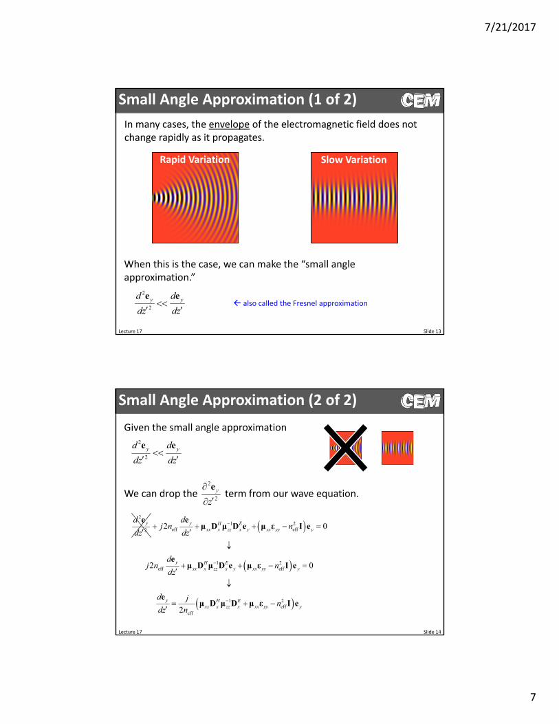
Small Angle Approximation (1 of 2)

When this is the case, we can make the “small angle approximation.”

2

2

y yd d

dz dz

e e

also called the Fresnel approximation

In many cases, the envelope of the electromagnetic field does not change rapidly as it propagates.

Rapid Variation Slow Variation

Lecture 17 Slide 14

Small Angle Approximation (2 of 2)

Given the small angle approximation2

2

y yd d

dz dz

e e

We can drop the           term from our wave equation.2

2

y

z

e

2

2

yd

dze

1 2eff eff

1 2eff eff

1 2eff

eff

2 0

2 0

2

y H Exx x zz x y xx yy y

y H Exx x zz x y xx yy y

y H Exx x zz x xx yy y

dj n n

dz

dj n n

dz

d jn

dz n

eμ D μ D e μ ε I e

eμ D μ D e μ ε I e

eμ D μ D μ ε I e

7/21/2017

8

Lecture 17 Slide 15

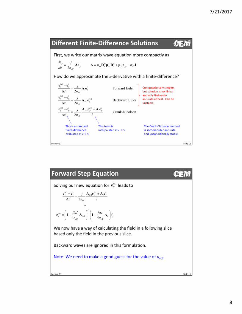
Different Finite‐Difference Solutions

How do we approximate the z‐derivative with a finite‐difference?

First, we write our matrix wave equation more compactly as

1 2eff

eff

2

y H Ey xx x zz x xx yy

d jn

dz n

e

Ae A μ D μ D μ ε I

1

eff

11

1eff

1 11

eff

Forward Euler2

Backward Euler2

Crank-Nicolson2 2

i iy y i

i y

i iy y i

i y

i i i iy y i y i y

j

z n

j

z n

j

z n

e eA e

e eA e

e e A e A e

This is a standard finite‐difference evaluated at i+0.5

This term is interpolated at i+0.5.

Computationally simpler, but solution is nonlinear and only first‐order accurate at best.  Can be unstable.

The Crank‐Nicolson method is second‐order accurate and unconditionally stable.

Lecture 17 Slide 16

Forward Step Equation

1 11

eff

1

11

eff eff

2 2

4 4

i i i iy y i y i y

i iy i i y

j

z n

j z j z

n n

e e A e A e

e I A I A e

Solving our new equation for        leads to1iye

We now have a way of calculating the field in a following slice based only the field in the previous slice.

Backward waves are ignored in this formulation.

Note: We need to make a good guess for the value of neff.

7/21/2017

9

Lecture 17 Slide 17

Implementationof 2D FD‐BPM

Lecture 17 Slide 18

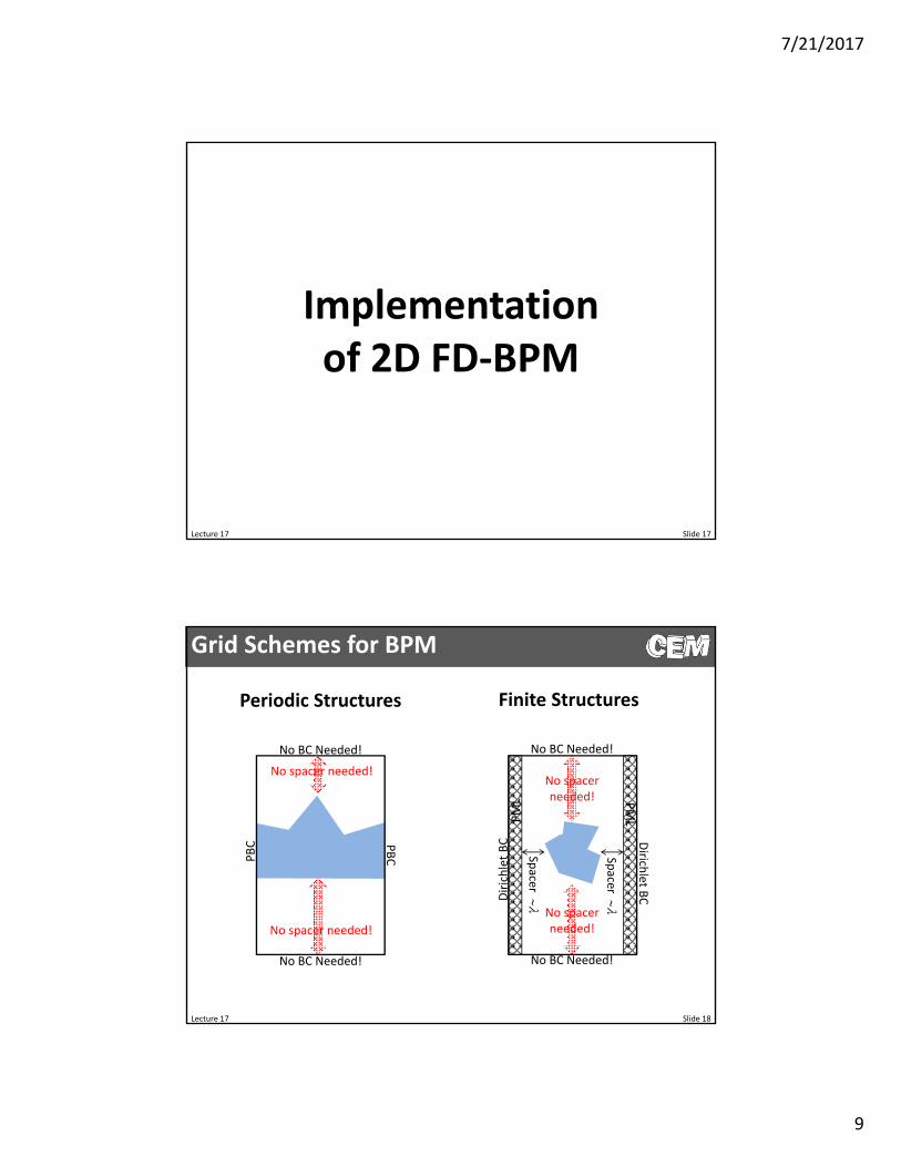
Grid Schemes for BPM

Periodic Structures Finite Structures

PBCP

BC

No BC Needed!

No BC Needed!

No BC Needed!

No BC Needed!

Dirich

letBCD

irichletBC

PMLP

ML

Spacer 

Spacer 

No spacer needed!

No spacer needed!No spacerneeded!

No spacerneeded!

7/21/2017

10

Lecture 17 Slide 19

The Effective Refractive Index, neffRecall the slowly varying envelop approximation.

eff eff, , , ,jn z jn zE x z x z e H x z x z e

The BPM does not calculate neff.  We must tell BPM what is neff.

How do we know neff without modeling the device?  

We have to calculate it or estimate it.

Techniques:

1. For plane waves and beams, calculate the average refractive index in the cross section of your grid to estimate the longitudinal wave vector.

2. For waveguide problems, calculate the effective index of your guided mode rigorously and use that in BPM.

Compute field in next plane

1 1i i i i e P e

Compute source at first plane

Ey(:,1) = ?;

Compute matrix derivative operators

and e hx xD D

Build deviceon grid

Calculate optimized grid

Lecture 17 Slide 20

Block Diagram of BPM

Define simulation parameters

Compute propagator P

1

1 1eff eff

12eff

4 4i i i i

i i i ih ei xx x zz x xx yy

j z j z

n n

n

P I A I A

A μ D μ D μ ε I

Post processDone?

Loop over z

BPM can handle modes, beams, plane waves, etc., very easily.

Extract slice & diagonalize. and i iμ ε

yes

no

Chooseneff

7/21/2017

11

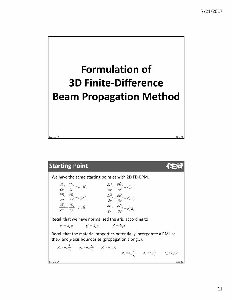
Lecture 17 Slide 21

Formulation of 3D Finite‐Difference 

Beam Propagation Method

Lecture 17 Slide 22

Starting Point

We have the same starting point as with 2D FD‐BPM.

yzxx x

x zyy y

y xzz z

EEH

y z

E EH

z xE E

Hx y

yzxx x

x zyy y

y xzz z

HHE

y z

H HE

z x

H HE

x y

Recall that we have normalized the grid according to

0x k x 0y k y 0z k z

Recall that the material properties potentially incorporate a PML at the x and y axis boundaries (propagation along z).

y xxx xx yy yy zz zz x y

x y

s ss s

s s

y xxx xx yy yy zz zz x y

x y

s ss s

s s

7/21/2017

12

Lecture 17 Slide 23

Slowly Varying Envelope Approximation

Assuming the field is not changing rapidly, we can write the field as

eff eff, , , ,jn z jn zE x z x z e H x z x z e

Maxwell’s equations become

Not a good approximation to make for metamaterials and photonic crystals!

Good for lenses, waveguides, etc.

eff

eff

yzy xx x

x zx yy y

y xzz z

jny z

jnz x

x y

eff

eff

yzy xx x

x zx yy y

y xzz z

jny z

jnz x

x y

yzxx x

x zyy y

y xzz z

EEH

y z

E EH

z xE E

Hx y

yzxx x

x zyy y

y xzz z

HHE

y z

H HE

z x

H HE

x y

Lecture 17 Slide 24

Matrix Form of Differential Equations

Each of these equations is written once for every point in the grid.  This large set of equations can be written in matrix form as

eff

eff

yey z y xx x

exx x z yy y

e ex y y x zz z

djn

dzd

jndz

eD e e μ h

ee D e μ h

D e D e μ h

eff

eff

yhy z y xx x

hxx x z yy y

h hx y y x zz z

djn

dzd

jndz

hD h h ε e

hh D h ε e

D h D h ε e

eff

eff

yzy xx x

x zx yy y

y xzz z

jny z

jnz x

x y

eff

eff

yzy xx x

x zx yy y

y xzz z

jny z

jnz x

x y

7/21/2017

13

Lecture 17 Slide 25

Eliminate Longitudinal Components

We solve the third equation in each set for the longitudinal components ez and hz.

1 e ez zz x y y x

h μ D e D e 1 h h

z zz x y y x

e ε D h D h

We now substitute these expressions into the remaining equations.

1eff

1eff

ye h hy zz x y y x y xx x

e h hxx x zz x y y x yy y

djn

dzd

jndz

eD ε D h D h e μ h

ee D ε D h D h μ h

1eff

1eff

yh e ey zz x y y x y xx x

h e exx x zz x y y x yy y

djn

dzd

jndz

hD μ D e D e h ε e

hh D μ D e D e ε e

Lecture 17 Slide 26

Rearrange Terms

We rearrange or remaining finite‐difference equations and collect the common terms.

1 1eff

1 1eff

e h e hxx x zz y x yy x zz x y

y e h e hy xx y zz y x y zz x y

djn

dzd

jndz

ee D ε D h μ D ε D h

ee μ D ε D h D ε D h

1 1eff

1 1eff

h e h exx zz y x yy x zz x y x

y h e h exx y zz y x y zz x y y

djn

dzd

jndz

hD μ D e ε D μ D e h

hε D μ D e D μ D e h

7/21/2017

14

Lecture 17 Slide 27

Block Matrix Form

We can now cast these four matrix equations into two block matrix equations.

1 1eff

1 1eff

e h e hxx x zz y x yy x zz x y

y e h e hy xx y zz y x y zz x y

djn

dzd

jndz

ee D ε D h μ D ε D h

ee μ D ε D h D ε D h

1 1eff

1 1eff

h e h exx zz y x yy x zz x y x

y h e h exx y zz y x y zz x y y

djn

dzd

jndz

hD μ D e ε D μ D e h

hε D μ D e D μ D e h

1 1

eff 1 1

e h e hx zz y yy x zz xx x x

e h e hy y y xx y zz y y zz x

djn

dz

D ε D μ D ε De e hP P

e e h μ D ε D D ε D

1 1

eff 1 1

h e h ex zz y yy x zz xx x x

h e h ey y y xx y zz y y zz x

djn

dz

D μ D ε D μ Dh h eQ Q

h h e ε D μ D D μ D

Lecture 17 Slide 28

Matrix Wave Equation

We derive the matrix wave equation by combining the two block matrix equations.   First, we solve the first block matrix wave equation for the magnetic field term.

1eff

x x x

y y y

djn

dz

h e eP

h e e

Second, we substitute this into the second block matrix equation.

1 1eff eff eff

22

eff eff eff2

2

2

x x x x x

y y y y y

x x x x x

y y y y y

x

d d djn jn jn

dz dz dz

d d djn jn n

dz dz dz

d

dz

e e e e eP P Q

e e e e e

e e e e ePQ

e e e e e

e

e 2eff eff2 x x

y y y

dj n n

dz

e eI PQ

e e

7/21/2017

15

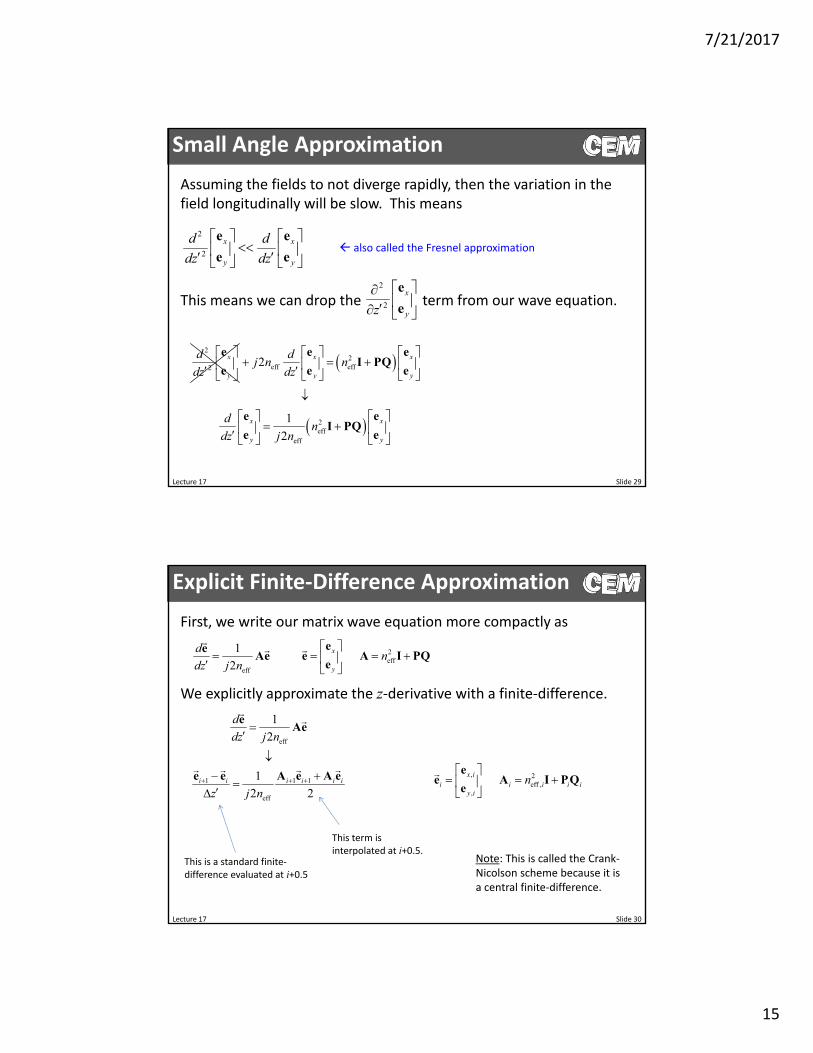
Lecture 17 Slide 29

Small Angle Approximation

Assuming the fields to not diverge rapidly, then the variation in the field longitudinally will be slow.  This means

2

2

x x

y y

d d

dz dz

e e

e e

This means we can drop the                 term from our wave equation.2

2

x

yz

e

e

also called the Fresnel approximation

2

2

x

y

d

dz

e

e

2eff eff

2eff

eff

2

1

2

x x

y y

x x

y y

dj n n

dz

dn

dz j n

e eI PQ

e e

e eI PQ

e e

Lecture 17 Slide 30

Explicit Finite‐Difference Approximation

We explicitly approximate the z‐derivative with a finite‐difference.

eff

1 1 1

eff

1

2

1

2 2i i i i i i

d

dz j n

z j n

eAe

e e A e A e

This is a standard finite‐difference evaluated at i+0.5

First, we write our matrix wave equation more compactly as

2eff

eff

1

2x

y

dn

dz j n

eeAe e A I PQ

e

, 2eff ,

,

x ii i i i i

y i

n

ee A I PQ

e

This term is interpolated at i+0.5.

Note: This is called the Crank‐Nicolson scheme because it is a central finite‐difference.

7/21/2017

16

Lecture 17 Slide 31

Forward Step Equation

1 1 1

eff

1

1 1eff eff

1

2 2

4 4

i i i i i i

i i i i

z j n

z z

j n j n

e e A e A e

e I A I A e

Solving our new equation for        leads to1ie

We now have a way of calculating the field in a following slice based only the field in the previous slice.

Backward waves are ignored in this formulation.

Note: We need to make a good guess for the value of neff.

Lecture 17 Slide 32

Alternative Formulationsof BPM

7/21/2017

17

Lecture 17 Slide 33

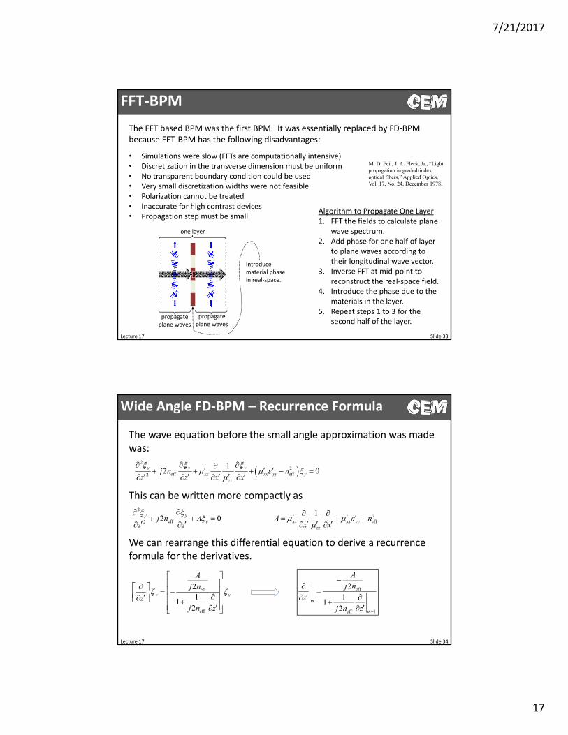
FFT‐BPM

The FFT based BPM was the first BPM.  It was essentially replaced by FD‐BPM because FFT‐BPM has the following disadvantages:

• Simulations were slow (FFTs are computationally intensive)• Discretization in the transverse dimension must be uniform • No transparent boundary condition could be used• Very small discretization widths were not feasible• Polarization cannot be treated• Inaccurate for high contrast devices• Propagation step must be small

one layer

propagate plane waves

propagate plane waves

Introduce material phase in real‐space.

Algorithm to Propagate One Layer1. FFT the fields to calculate plane 

wave spectrum.2. Add phase for one half of layer 

to plane waves according to their longitudinal wave vector.

3. Inverse FFT at mid‐point to reconstruct the real‐space field.

4. Introduce the phase due to the materials in the layer.

5. Repeat steps 1 to 3 for the second half of the layer.

M. D. Feit, J. A. Fleck, Jr., “Light propagation in graded-index optical fibers,” Applied Optics, Vol. 17, No. 24, December 1978.

Lecture 17 Slide 34

Wide Angle FD‐BPM – Recurrence Formula

The wave equation before the small angle approximation was made was:

2

2eff eff2

12 0y y y

xx xx yy yzz

j n nz z x x

This can be written more compactly as2

2eff eff2

12 0 y y

y xx xx yyzz

j n A A nz z x x

We can rearrange this differential equation to derive a recurrence formula for the derivatives.

eff

eff

21

12

y y

A

j n

zj n z

eff

1eff

21

12

m

m

Aj n

zj n z

7/21/2017

18

Lecture 17 Slide 35

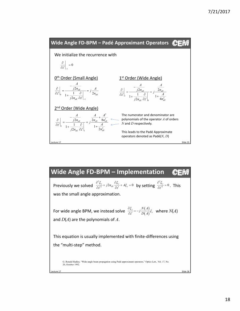
Wide Angle FD‐BPM – Padé Approximant Operators

We initialize the recurrence with

1

0z

0th Order (Small Angle)

eff

0 eff

1eff

21 2

12

Aj n A

jz n

j n z

1st Order (Wide Angle)

eff eff

12eff0eff

2 21 11

42

A Aj n n

jAznj n z

2nd Order (Wide Angle)2

3eff eff eff

22eff1eff

2 2 81 11

22

A A Aj n n n

jAznj n z

The numerator and denominator are polynomials of the operator A of orders N and D respectively.

This leads to the Padé Approximate operators denoted as Padé(N, D)

Lecture 17 Slide 36

Wide Angle FD‐BPM – Implementation

Previously we solved                                         by setting              .  This 

was the small angle approximation.

For wide angle BPM, we instead solve                             where N(A) 

and D(A) are the polynomials of A.

This equation is usually implemented with finite‐differences using 

the “multi‐step” method.

2

eff22 0y y

yj n Az z

2

20y

z

yy

N Aj

z D A

G. Ronald Hadley, “Wide-angle beam propagation using Padé approximant operators,” Optics Lett., Vol. 17, No. 20, October 1992.

7/21/2017

19

Lecture 17 Slide 37

Bi‐Directional BPM

The beam propagation method inherently propagates waves in only the forward direction.

It is possible to modify the method so as to account for backward scattered waves.

This is accomplished in a manner similar to how we derived scattering matrices.

By the time BPM is modified to be bidirectional and wide‐angle, it approaches being a rigorous method.  The implementation, however, is tedious.  At this point, use the method of lines which is fully rigorous and has a simpler implementation.

Hatem El-Refaei, David Yevick, and Ian Betty, “Stable and Noniterative Bidirectional Beam Propagation Method,” IEEE Photonics Technol. Lett, Vol. 12, No. 4, April 2000.