LECTURE 16: LEARNING THEORY

CS446 Introduction to Machine Learning (Spring 2015) University of Illinois at Urbana-Champaign http://courses.engr.illinois.edu/cs446

Prof. Julia Hockenmaier [email protected]

LECTURE 16: LEARNING THEORY

CS446 Machine Learning

Learning theory questions – Sample complexity:

How many training examples are needed for a learner to converge (with high probability) to a successful hypothesis?

– Computational complexity: How much computational effort is required for a learner to converge (with high probability) to a successful hypothesis?

– Mistake bounds: How many training examples will the learner misclassify before converging to a successful hypothesis?

2

PAC learning (Probably Approximately Correct)


Terminology/Assumptions The instance space X is the set of all instances x. Assume each x is of size n. Instances are drawn i.i.d. from an unknown probability distribution D over X: x ~ D A concept c: X → {0,1} is a Boolean function (it identifies a subset of X) A concept class C is a set of concepts The hypothesis space H is the (sub)set of Boolean functions considered by the learner L We evaluate L by its performance on new instances drawn i.i.d. from D

4

What can a learner learn? We can’t expect to learn concepts exactly: –  Many concepts may be consistent with the data –  Unseen examples could have any label

We can’t expect to always learn close approximations to the target concept: –  Sometimes the data will not be representative

We can only expect to learn with high probability a close approximation to the target concept.

5

PAC Learning – Intuition Recall the conjunction example. We have seen many examples (drawn from D ) If x1 was active in all positive examples we have seen, it is very likely that it will be active in future positive examples In any case, x1 is active only in a small percentage of the examples so our error will be small

6

-

True error of a hypothesis

7

Instance space X

f h + +

−

−

-

ErrorD = x∈P D[ f (x) ≠ h(x)]

f and h disagree


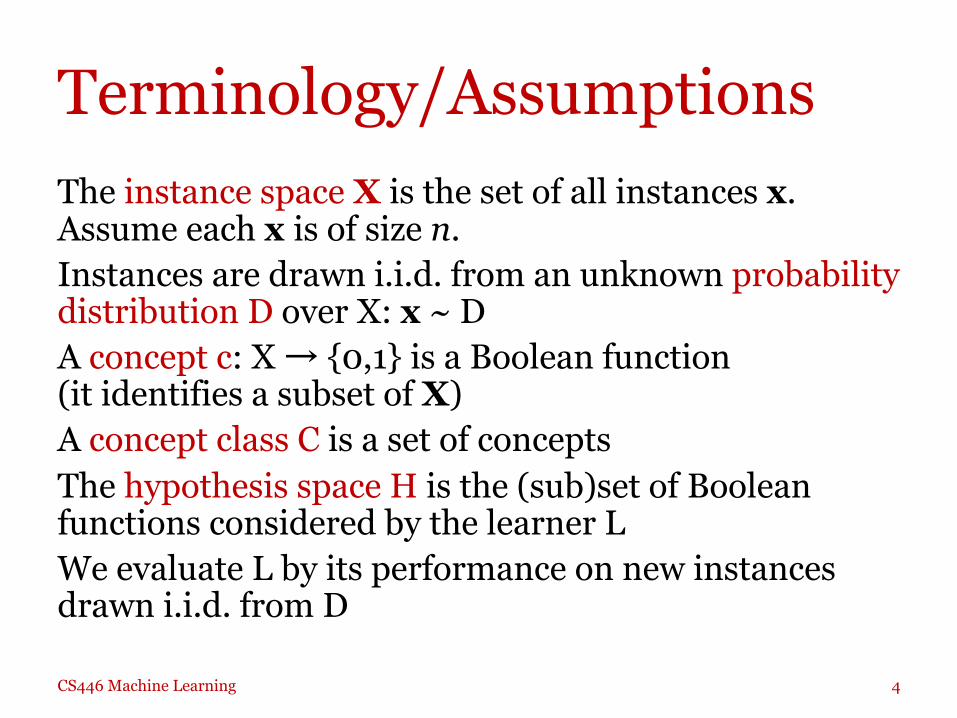
True error of a hypothesis The true error (errorD(h)) of hypothesis h with respect to target concept c and distribution D is the probability that h will misclassify an instance drawn at random according to D:

errorD(h) = Px~D(c(x) ≠ h(x)) Can we bound the error based on what we know from the training data?

8


What is the error for learning conjunctions? p(z): prob. that z = 0 in a positive example Claim: h only makes mistakes on positive examples. A mistake is made only if a literal z that is in h but not in the target f is false in a positive example. In this case, h will say NEG, but the example is POS.

Thus, p(z) is also the probability that z causes h to make a mistake on a randomly drawn example. Hence, Error(h) ≤∑zP(z)

9

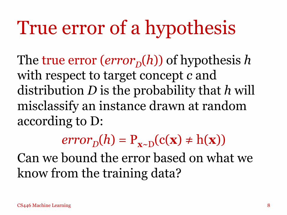
Learning Conjunctions– Analysis Call a literal z bad if p(z) > ε/n. A bad literal has a significant probability to appear with a positive example but, nevertheless, it has not appeared with one in the training data. Claim: If there are no bad literals, than error(h) < ε. Reason: What if there are bad literals ? –  Let z be a bad literal. –  What is the probability that z will not be eliminated by one example? Pr(z survives one example) = 1- Pr(z is eliminated by one example) = 1 – p(z) < 1- ε/n The probability that z will not be eliminated by m examples is therefore: Pr(z survives m independent examples) = (1 –p(z))m < (1- ε/n)m

There are at most n bad literals, so the probability that some bad literal survives m examples is bounded by n(1- ε/n)m

10

Learning Conjunctions– Analysis We want this probability to be small. Say, we want to choose m large enough such that the probability that some bad z survives m examples is less than δ. Pr(z survives m example) = n(1- ε/n)m < δ Using 1-x < e-x it is sufficient to require that n e-mε/n < δ Therefore, we need m examples to guarantee a probability of failure (error > ε) of less than δ. With m examples, the probability that there are no bad literals is > 1-δ With δ=0.1, ε=0.1, and n=100, we need 6907 examples. With δ=0.1, ε=0.1, and n=10, we need 460 example, only 690 for δ=0.01

11

)}/1ln(){ln( δε

+> nnm


PAC learnability Consider: –  A concept class C over a set of instances X

(each x is of length n) –  A learner L that uses hypothesis space H C is PAC-learnable by L if for all c∈ C and any distribution D over X, L will output with probability at least (1−δ) and in time that is polynomial in 1/ε, 1/δ, n and size(c), a hypothesis h ∈ H with errorD(h) ≤ ε (for 0 < δ < 0.5 and 0 < ε < 0.5)

12


PAC learnability in plain English

– With arbitrarily high probability (p=1−δ), L must output a hypothesis h that has arbitrarily low error ε.

– L must learn h efficiently (using a polynomial amount of time per example, and a polynomial number of examples)

13

PAC learning: intuition

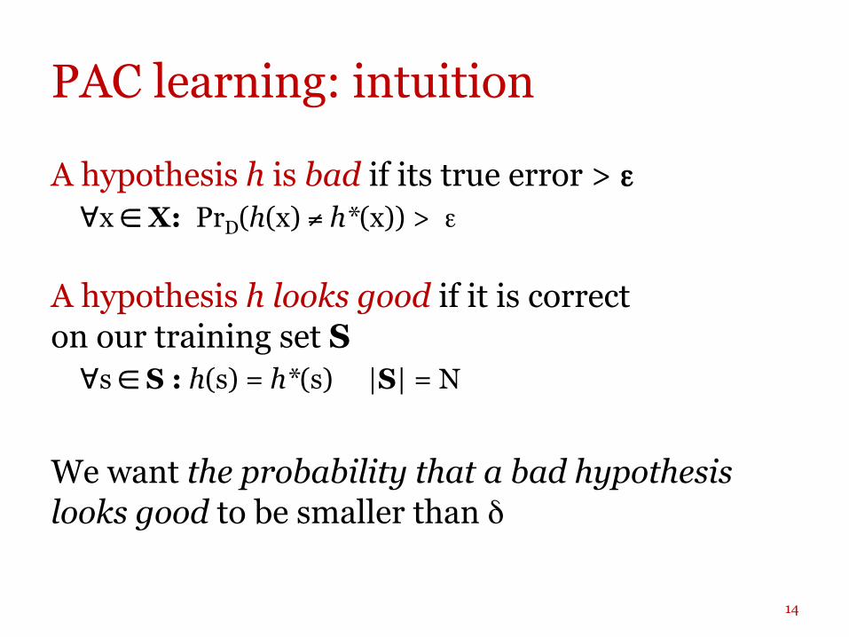
A hypothesis h is bad if its true error > ε ∀x ∈ X: PrD(h(x) ≠ h*(x)) > ε

A hypothesis h looks good if it is correct on our training set S ∀s ∈ S : h(s) = h*(s) |S| = N

We want the probability that a bad hypothesis looks good to be smaller than δ

14

PAC learning: intuition

We want the probability that a bad hypothesis looks good to be smaller than δ Probability of one bad h getting one x ~ XD correct:

PD(h(x) = h*(x)) ≤ 1-ε

Probability of one bad h getting m x ~ XD correct: PD(h(x) = h*(x)) ≤ (1-ε)m

Prob’ty that any h gets m x~XD correct: ≤ ∣H∣(1-ε)m Exclusive union bound: P(A ∨ B) ≤ Pr(A) + Pr(B) Set ∣H∣(1-ε)m ≤ δ, solve for m

15


Sample complexity (for finite hypothesis spaces and consistent learners)

Consistent learner: returns hypotheses that perfectly fit the training data (whenever possible).

16


Version space VSH,D

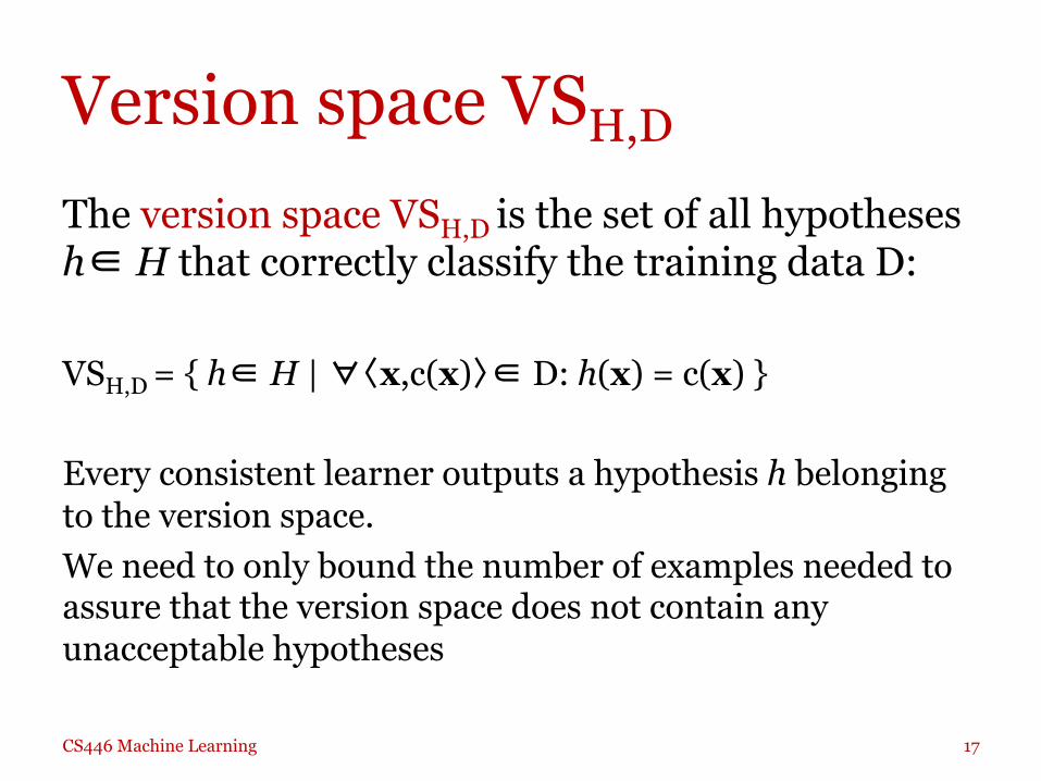
The version space VSH,D is the set of all hypotheses h∈ H that correctly classify the training data D: VSH,D = { h∈ H | ∀〈x,c(x)〉∈ D: h(x) = c(x) } Every consistent learner outputs a hypothesis h belonging to the version space. We need to only bound the number of examples needed to assure that the version space does not contain any unacceptable hypotheses

17


Sample complexity (finite H) –  The version space VSH,D is said to be ε-exhausted with

respect to concept c and distribution D if every h∈ VSH,D has true error < ε with respect to c and distribution D

–  If H is finite, and the data D is a sequence of m i.i.d. samples of c, then for any 0 ≤ ε ≤ 1, the probability that VSH,D is not ε-exhausted with respect to c is ≤ |H|e-εm

–  #training examples required to reduce probability of failure below δ: Find m such that |H|e-εm < δ

–  So, a consistent learner needs m ≥ 1/ε (ln |H| + ln(1/δ)) examples to get an error below δ (often an overestimate; |H| can be very large)

18

Occam’s Razor (1) Claim: The probability that there exists a hypothesis h ∈ H that (1) is consistent with m examples and (2) satisfies error(h) > ε ( ErrorD(h) = Prx 2 D [f(x) !=h(x)] ) is less than |H|(1- ε )m .

19

Occam’s Razor (1) Proof: Let h be a bad hypothesis. Probability that h is consistent with one example f(x): Px~D(f(x) = h(x)) < 1−ε Since the m examples are drawn independently, the probability that h is consistent with all m examples is less than (1−ε)m The probability that some hypothesis in H is consistent with m examples is smaller than |H|(1−ε)m 20

Note that we don’t need a true f for this argument; it can be done with h, rela:ve to a distribu:on over X £ Y.


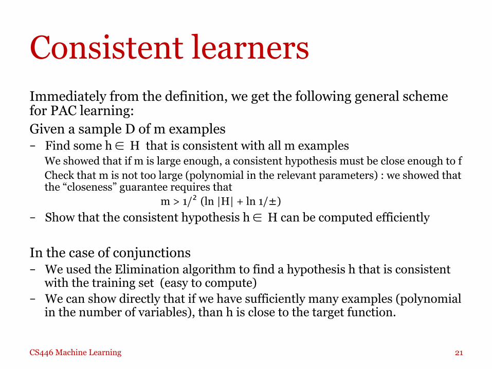
Consistent learners Immediately from the definition, we get the following general scheme for PAC learning: Given a sample D of m examples –  Find some h ∈ H that is consistent with all m examples

We showed that if m is large enough, a consistent hypothesis must be close enough to f Check that m is not too large (polynomial in the relevant parameters) : we showed that the “closeness” guarantee requires that

m > 1/² (ln |H| + ln 1/±) –  Show that the consistent hypothesis h ∈ H can be computed efficiently In the case of conjunctions –  We used the Elimination algorithm to find a hypothesis h that is consistent

with the training set (easy to compute) –  We can show directly that if we have sufficiently many examples (polynomial

in the number of variables), than h is close to the target function.

21


Vapnik-Chervonenkis (VC) dimension

22

Infinite Hypothesis Space The previous analysis was restricted to finite hypothesis spaces Some infinite hypothesis spaces are more expressive than others –  E.g., Rectangles, vs. 17- sides convex polygons vs.

general convex polygons –  Linear threshold function vs. a conjunction of LTUs Need a measure of the expressiveness of an infinite hypothesis space other than its size The Vapnik-Chervonenkis dimension (VC dimension) provides such a measure. Analogous to |H|, there are bounds for sample complexity using VC(H)


VC dimension (basic idea) The VC dimension of a hypothesis space H measures the complexity of H by the number of distinct instances from X that can be completely discriminated (‘shattered’) using H, not by the number of distinct hypotheses (|H|).

24


VC dimension (basic idea) An unbiased hypothesis space H shatters the entire instance space X (is able to induce every possible partition on the set of all possible instances) The larger the subset X that can be shattered, the more expressive a hypothesis space is, i.e., the less biased.

25


Shattering a set of instances A set of instances S is shattered by the hypothesis space H if and only if for every dichotomy of S there is a hypothesis h in H that is consistent with this dichotomy. –  dichotomy: partition instances in S into + and – –  one dichotomy = label all instances in a subset P⊆ S as +, and instances in the complement of P, S\P as –

The ability of H to shatter S is a measure of its capacity to represent concepts over S

26

Instances: Real numbers Hypothesis space: Intervals [a, b] defines the positive instances We can shatter any dataset of two reals, but we cannot shatter datasets of three reals


Shattering

27

- - + a b


VC dimension of H The VC dimension of the hypothesis space H, VC(H), is the size of the largest finite subset of the instance space X that can be shattered by H. If arbitrarily large finite subsets of X can be shattered by X then VC(H) = ∞

28

VC Dimension The VC dimension of hypothesis space H over instance space X is the size of the largest finite subset of X that is shattered by H. – If there exists one (or more) subsets of size

d that can be shattered, then VC(H) ≥ d – If no subset of size d can be shattered,

then VC(H) < d

29

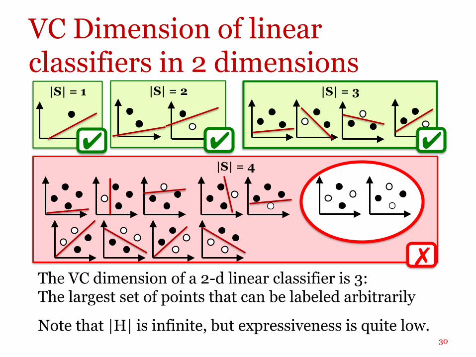
|S| = 4

|S| = 2 |S| = 1

VC Dimension of linear classifiers in 2 dimensions

The VC dimension of a 2-d linear classifier is 3: The largest set of points that can be labeled arbitrarily

Note that |H| is infinite, but expressiveness is quite low. 30

|S| = 3

✔

✗

✔ ✔


VC dimension if H is finite If H is finite: VC(H) ≤ log2|H| – A set S with d instances has 2d distinct

subsets/dichotomies. – Hence, H requires 2d distinct hypotheses

to shatter d instances. – If VC(H) = d: 2d ≤ |H|

hence: VC(H) = d ≤ log2|H|

31

COLT Conclusions The PAC framework provides a reasonable model for theoretically analyzing the effectiveness of learning algorithms. The sample complexity for any consistent learner using the hypothesis space, H, can be determined from a measure of H’s expressiveness (|H|, VC(H)) If the sample complexity is tractable, then the computational complexity of finding a consistent hypothesis governs the complexity of the problem. Sample complexity bounds given here are far from being tight, but separates learnable classes from non-learnable classes (and show what’s important). Computational complexity results exhibit cases where information theoretic learning is feasible, but finding good hypothesis is intractable. The theoretical framework allows for a concrete analysis of the complexity of learning as a function of various assumptions (e.g., relevant variables)

LECTURE 16: LEARNING THEORY

Documents