Lecture 16: Collective Action Lecture 1

14.75: Collective Action Lecture 1

Ben Olken

Olken () Collective Action Lecture 1 1 / 47

Collective Action

Each of you has $5 You can choose how much to keep and how much to put into the pot. You put c into the pot and keep $5 − c . I will triple whatever is in the pot, and then divide it back among all of you. I will randomly select one of you to be the winner. If you are the winner, you will get paid

5 − ci + 3 × 1 ∑ cjN j

Clear? We will do this 5 times, and then I’ll randomly select one of the 5 rounds, and 1 person, and pay them. For each round, please write your name, round number, and contribution on it. The class will only know the distribution of contributions but they will be anonymous. (We need your name to pay you).


Discussion

What did you observe?


Overview

Collective action failures stem from misalignment of private and collective incentives In the developing world, this manifests itself in many ways. Thoughts?

Insuffi cient provision of local public goods Roads, schools, health clinics, security, forest protection, etc

Insuffi cient monitoring of local offi cials Teachers and health workers not coming to work Local offi cials stealing funds from central government projects

How does this relate to the experiment we just did?


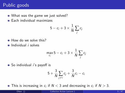
Public goods

What was the game we just solved? Each individual maximizes

5 − ci + 3 × 1 ∑ cjN j

How do we solve this? Individual i solves

max 5 − ci + 3 × 1 ∑ cjci N j

So individual i’s payoff is 3 3

5 + ∑ cj + ci − ciN Nj =i

This is increasing in ci if N < 3 and decreasing in ci if N > 3. Olken () Collective Action Lecture 1 5 / 47

Public goods

So if N < 3 the equilibrium is? If N > 3 the equilibrium is? What about if N = 3? Why do contributions depend on N? What about total contributions? Total contributions are Nci .

If N < 3, total contributions are increasing in N. If N > 3, total contributions are 0.


Interior solutions

Note that in the previous model the first order condition was always positive or negative — so you always contributed either everything or nothing (or were indifferent) We can easily make the model smooth by changing the objective function a bit Now suppose that I will rebate to everyone

3 ∑ √

cjN j

so each individuals payoff is

3 √5 − ci + ∑ cjN j

How is this different? Olken () Collective Action Lecture 1 7 / 47

Interior solutions

3 √5 − ci + ∑ cjN j

The marginal return for individual i is

3 1 √ − 12N ci

So as ci → 0 the marginal return goes to ∞. So, you’ll always contribute something.


Interior solutions

Solving this model, we have that the FOC is

3 1 √ − 1 = 02N ci

3 1 √ = 12N ci

√ 3 ci =

2N 23 ci =

2N


Interior solutions

23 ci =

2

N

Total contributions are

Nci = N 3 2N

2

Nci = 3 2

2

So in this model, total contributions


( )

( )( )

1

decrease with N.

N

Interior solutions

Are you sensing any patterns about contributions? The idea that contributions per

individual

fall as N increases is a very general feature of these types of models. The reason is that a given individuals’marginal return from contributing is decreasing in N. However, what happens to total contributions — Ncj — is in general ambiguous and depends on the model. Just depends on whether

1 1contributions fall with N faster than or slower than N .N


individual

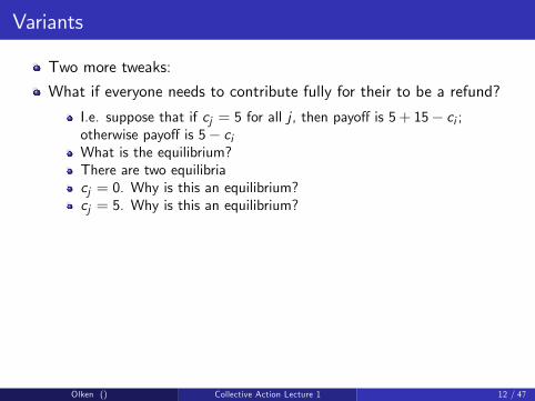
Variants

Two more tweaks: What if everyone needs to contribute fully for their to be a refund?

I.e. suppose that if cj = 5 for all j , then payoff is 5 + 15 − ci ; otherwise payoff is 5 − ci What is the equilibrium? There are two equilibria cj = 0. Why is this an equilibrium? cj = 5. Why is this an equilibrium?


Variants

What if we need at least k people to contribute fully for their to be a refund?

I.e. suppose that if cj = 5 for at least k individuals, then payoff is 5 + 15 − ci ; otherwise payoff is 5 − ci What is the equilibrium? There are two pure strategy equilibria cj = 0 for everyone. Why is this an equilibrium? cj = 5 for k people and cj = 0 for everyone else. Why is this an equilibrium?

In reality, which do you think is easier to harder to organize?


A slightly more general model Banerjee, Iyer, and Somanathan (2007)

Olson (1965): "the larger the group, the less it will be able to favor its common interests." Let

n n f ( ∑ ai ) = [ ∑ ai ]α , 0 < α < 1

be the probability that a particular collective effort succeeds. ai is the effort of group member i , and assume that there are n group members. Let everyone benefit an amount b from the success of the effort. Let the cost of the effort be v (a) = aβ , β > 1. Then a group member will maximize

n b[ ∑ β ai ]α − ai

Then ai will satisfy n

αb[ ∑ β−1 ai ]α−1 = βai Olken () Collective Action Lecture 1 14 / 47

Collective action and group size

So in equilibrium β−1αb[na]α−1 = βa1−α β−ααb = βn a

Denote Ae = na, the total equilibrium collective effort. Then

αb = βn1−αaβ−α

αnβ−1b = β(Ae )β−α

αnβ−1b β

= (Ae )β−α

Ae = αnβ−1b 1

β−α

β β−1

Ae = kn β−α

So Ae — total group effort — is increasing in n since β > 1 and 0 < α < 1.


( )

Optimal effort

Recall that an individual group member maximizes

n β ai ]α − ab[ ∑ i

By contrast, the socially optimal choice of effort maximizes

n n nb[ ∑ ai ]α −∑ β ai

How is this different? This tells us that

β−1nαb[na]α−1 = βa

Hence the optimal social effort Ao satisfies

αnβb = β(Ao )β−α


Optimal vs. actual effort

Recall αnβ−1b = β(Ae )β−α

and αnβb = β(Ao )β−α

Which implies 1 Ae β−α =

n Ao

Hence Ae /Ao goes to zero as n goes to infinity.


( )

Implications

As before, collective action is harder per capita in larger groups because the misalignment of private and social incentives is larger. In this model however Ae is always increasing in n. To get at the possibility that Ae is actually declining in n, one option is to bring in the idea that smaller groups have higher stakes per capita. In other words we now introduce the idea that there is some private component in the returns from collective action.


Adding crowd-out

A group member will now maximize nw β

(b + )[ ∑ ai ]α − ain

So in equilibrium

w β−1α(b + )[na]α−1 = βan

and w α(b + )[n]β−1 = β(Ae )β−α

n Clearly increasing n has two effects and the result can go either way

(e.g., b = 0 and β < 2 reverses the previous result)

Intuitively there is more of a free rider problem in big groups but the bigger group has to put in less effort per capita to get to the same total effort.


Collective action and heterogeneity

There is a few that it is harder to have collective action in heterogenous groups. Why might this be? We will explore several models of heterogeneity Suppose there are m groups each of size nj . mnj = n Assume that once again the public good has a public component and a private component, where private means that some group captures it. What might this be? E.g. location of a public good


� �


The probability of it being captured by group J conditional on the public good being built is

∑ ai i ∈J

∑ ai The payoff function is then

∑ ai i ∈J β

(b + w )[∑ ai ]α − a∑ ai i

� �α � �α−1 β = b ∑ ai + w ∑ ai ∑ ai − ai

i ∈J


� �


At the optimum we will have

αb[∑ ai ]α−1 + [∑ ai ]α−1w

−(1 − α) ∑ ai [∑ ai ]α−2w i ∈J

β−1 = βai

or

αbAα−1 + Aα−1w − (1 − α) A [A]α−2w

m β−1

= βai

or

+ Aα−1 1 [A]α−1αbAα−1 w − (1 − α) w

m = β(A/n)β−1


[ ]


Recall that keeping n fixed, increasing m increases heterogeneity. We just showed that

αbAα−1 + Aα−1w − (1 − α) 1 [A]α−1w = β(A/n)m

αb + w − (1 − α) 1 w = β(A/n)β−1A1−α m

So increasing m increases the left hand side of the equation. To balance, A must also increase. This shows that increasing m (i.e., increasing heterogeneity) increases A. Heterogeneity helps!Intuition? The intuition in this model is that the groups are competing with one another to capture the good, and the smaller each group is, the more you have an incentive to work.



Intuition: Group size in this framework matters only because your incentive to put in effort depends in part on what is happening in your group and bigger groups discourage effort. So having smaller groups increases effort.

In order to capture the intuition that heterogeneity hurts, we need to look for a context where the free-rider problem is not the big problem. Instead, we’ll look at a context where the problem is heterogeneity in tastes


" "

Key distinction between this model and the previous model: now there is a type of public good, not just an amount of public good Individual i utility function given by

ui = g α (1 − li ) + y − t

where g is amount of public good, and li is distance between individual’s most preferred type of public good and the actual type of public good, y is income, and t is lump-sum taxes used to finance the public good. Assume 0 < α < 1. Normalize population size to one, so g = t Rewrite utility as

ui = g α (1 − li ) + y − g

Assume voters vote first on size of public good, and then vote on the type of the public good. In the second stage, type of good is the one preferred by the median voter.


Collective action and heterogeneityAlesina, Baqir, and Easterly (1999): "Public Goods and Ethnic Divisions"

� �

� �


How does this affect amount of public good? Individual i solves

αmax g 1 − ̂li + y − g

where l̂i is the distance of individual i from the ideal type of the median voter. Solution is 1 ∗ 1−αg = α 1 − ̂lii

Define l̂m as the median distance from the type most preferred by i median voter. ("median distance from the median"). Then amount of public good is given by 1 ∗ 1−αg = α 1 − ̂lm

i i

This implies that equilibrium amount of public good is decreasing in l̂m i . Polarization increases this distance.


[ ]

[ ]

Illustration Low heterogeneity

1250 QUARTERLY JOURNAL OF ECONOMICS

COROLLARY. The equilibrium amount of public good is decreasing I

in lI, the median distance from the median.

The median distance from the median can be considered an indicator of polarization of preferences, as illustrated in Figure I. Panel (a) shows a case of low median distance from the median; panel (b) shows a case of a larger median distance from the median. The picture of panel (b) is an example of a polarized society, with two separate groups with relatively homogeneous

a)

Median Distance F from the Median

MEDIAN

b) Median Distance from the Median

FIGURE I Examples of Different "Median Distances from the Median"


Image removed due to copyright restrictions. See: Alesina, Alberto, Reza Baqir, et al. "Public Goodsand Ethnic Divisions." Quarterly Journal of Economics 114, no. 4 (1999): 1243-84.Figure I Examples of Different "Median Distances from the Median."

" "

Setting: US school districts Idea: political jurisdictions are formed from a trade-off of economies of scale and homogeneity. So number of school districts in a county is:

Increasing in county size Increasing in fixed costs measures Decreasing in heterogeneity


EvidenceAlesina, Baqir, and Hoxby 2004: "Political Jurisdictions in Heterogeneous Communities"

OLS results with state fixed effects


and panel data.

Images from Alesina, Alberto, Reza Baqir, et al . "Political Jurisdictions in Heterogeneous Communities."Journal of Political Economy 112, no. 2 (2004): 348-96. Removed:Table 2 "Effect of Population Heterogeneity on the Number of School Districts in a County Dependent Variable: ln(Number of School Districts in a County)" fromFig 2. Does racial heterogeneity prevent districts from consolidating?Table 5 Effect of Changes in Population Heterogeneity on Changes in the Number of School Districts in a Countybetween 1990 and 1960 Dependent Variable: Change in ln(Number of School Districts in a County), 1990 - 1960

""

Setting: school funding and facilities in rural Kenya Slightly different theoretical motivation:

They posit no preference heterogeneity over these types of goods Instead, they think about voluntary contributions (not compulsory taxes), with social sanctions for non-payment Assume no ability to impose social sanctions across ethnic groups

Empirical approach: Low residential mobility implies that ethnic heterogeneity is exogenously determined with respect to public goods provision (e.g., no sorting) Compare contributions cross-sectionally


Evidence from KenyaMiguel and Gugerty (2005): "Ethnic diversity, social sanctions, and public goods inKenya"

How to measure heterogeneity

How do they measure heterogeneity? A common metric is the probability that two randomly drawn individuals will be from two different ethnic groups, denoted ethnolinguistic fractionalization. Define the proportion of individuals in ethnic group e as pe Then heterogeneity is denoted by

2ELF = 1 − ∑ (pe )e


Results

Table 5

Ethnic diversity and local primary school funding

Explanatory

variable

Dependent variable

School

ELF

across

tribes

Total local primary school funds collected per pupil in 1995 (Kenyan Shillings)

(1)

OLS

1st stage

(2)

OLS

(3)

OLS

(4)

IV-2sls

(5)

OLS

(6)

OLS

(7)

OLS

(8)

Spatial

OLS

(9)

Spatial

OLS

Ethnic diversity measures

Zonal ELF

across tribes

0.86***

(0.07)

�185.7**

(77.9)

�145.2***

(49.6)

�143.6*

(82.1)

School ELF

across tribes

�32.9

(64.0)

�216.4**

(88.4)

1-(Proportion

largest ethnic

group in zone)

�162.9**

(66.6)

ELF across tribes

for all schools

within 5 km

�174.0**

(76.3)

�174.0**

(80.8)

Zonal controls

Proportion fathers

with formal

employment

189.5

(165.1)

�220.6*

(120.5)

184.6

(170.9)

142.8

(167.3)

Proportion of pupils

with a latrine

at home

�431.6***

(139.9)

�286.3

(228.0)

�429.8***

(150.3)

�466.9

(250.2)

Proportion livestock

ownership

120.1

(136.9)

186.2

(130.4)

110.6

(148.3)

116.9

(117.7)

Proportion cultivates

cash crop

35.7

(61.4)

22.2

(106.9)

27.8

(62.4)

85.2

(78.4)

Proportion Teso pupils 67.9

(181.4)

Geographic division

indicators

No No No No No Yes No No No

Root MSE 0.14 99.8 96.7 105.5 95.0 93.0 95.4 97.1 95.0

R2 0.40 0.00 0.06 – 0.14 0.25 0.12 0.06 0.09

Number of schools 84 84 84 84 84 84 84 84 84

Mean dependent

variable

0.20 152.6 152.6 152.6 152.6 152.6 152.6 152.6 152.6

are

(of the seven) regression 4 is zonal ELF

E. Miguel, M.K. Gugerty / Journal of Public Economics 89 (2005) 2325–2368 2351


Courtesy of Elsevier. Used with permission.

" "

How prevalent are these types of collective action problems in developing countries? Olken and Singhal (forthcoming) study phenomenon of ’voluntary’ contributions to local public goods

Harambee in Kenya Gotong Royong in Indonesia and see Ostrom (1991) for more

Use micro data from 10 countries to establish some stylized facts


Informal taxationOlken and Singhal (2011): "Informal Taxation"

Stylized facts Magnitude

Participation rates are 20% or higher in all surveyed countries (except Albania) and exceed 50% in Ethiopia, Indonesia, and Vietnam Participation rates are always higher in rural areas

Between 27% and 183% higher, depending on country

A substantial share of households (10-76%) make in-kind payments in labor

Average labor payments range from 0.2 days per year (Albania) to 14.1 days per year (Ethiopia)


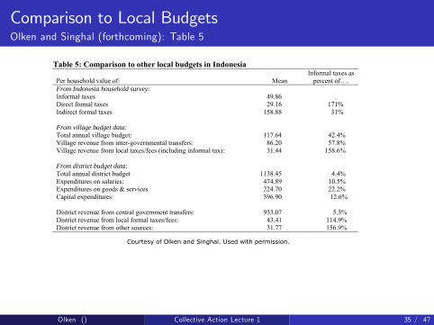
Comparison to Local Budgets Olken and Singhal (forthcoming): Table 5

36

Table 5: Comparison to other local budgets in Indonesia

Per household value of: Mean Informal taxes as

percent of…. From Indonesia household survey: Informal taxes 49.86 . Direct formal taxes 29.16 171% Indirect formal taxes 158.88 31% From village budget data: Total annual village budget: 117.64 42.4% Village revenue from inter-governmental transfers: 86.20 57.8% Village revenue from local taxes/fees (including informal tax): 31.44 158.6%

From district budget data: Total annual district budget 1138.45 4.4% Expenditures on salaries: 474.89 10.5% Expenditures on goods & services 224.70 22.2% Capital expenditures: 396.90 12.6% District revenue from central government transfers: 933.07 5.3% District revenue from local formal taxes/fees: 43.41 114.9% District revenue from other sources: 31.77 156.9%


Courtesy of Olken and Singhal. Used with permission.

Is it voluntary?

In Indonesia survey, asked questions about: Who decides whether a household should pay Who decides amount each household should pay Formal sanctions (if any) for failure to pay specified amount

Results: Only 8% of households report that they decide whether to pay; 84% say village/neighborhood head decides Only 20% of households report that they decide how much to pay; 69% say village/neighborhood head decides 38% report an offi cial sanction for failing to pay — typically replace with someone else, give materials instead, or pay a fine.

Higher income people have higher probability of reporting sanctions for failure to pay

Suggests these types of semi-formal contributions are an important part of the story for local public goods — and that social sanctions are used to overcome the free rider problem


Does "social capital" matter?

Miguel and Gugerty and Olken and Singhal papers suggest that these contributions are enforced through "social sanctions" This is connected to a broader idea, that "social capital" is an important supporter of collective action

E.g., Putnam — "Making Democracy Work" and "Bowling Alone" Could be because people trust each other (with trust enforced through links on social network) Could be because social links are a way to exclude people who fail to participate


" "

Setting: Examines the impact of television (and radio) on social capital in over 600 Indonesian villages Main source of identification: plausibly exogenous variation in signal strength associated with the mountainous terrain of East / Central Java Additional sources of identification:

Compare social capital in subdistricts before and after introduction of private television in 1993 Use model of electromagnetic signal propagation to explicitly isolate impact of topography

Then: examine the impact of television reception on corruption in road projects


Testing social capital’s impact using TVOlken (2009): "Does TV and Radio Destroy Social Capital?"

Map: Variation in television reception


Setting

Indonesian villages have extremely dense social networks Typical Javanese village of 2,600 adults has 179 groups of various types Types of groups: Neighborhood associations, religious study groups, ROSCAs, health and women’s groups, volunteer work

Television and radio 80 percent of rural households watch TV per week in 2003 11 national TV stations, showing mix of news, soap operas, movies, etc Broadcasting centered around major cities But prior to 1991, only 1 TV channel (gov’t channel) Will not separately identify TV and radio as I don’t have independent data on radio, and they are likely co-linear in any case


Does better reception translate into increased use?

Show that in Central / East Java sample, television reception is orthogonal to a large number of village characteristics Estimate impact of channels on use at individual level with data from East / Central Java survey:

MINUTEShvsd = αd + NUMCHANsd

+Yhvsd γ + Xvsd δ1 + δ2ELEVATIONsd + εhvsd

where: MINUTEShvsd is number of minutes respondent spends watching TV or listening to radio Yhvsd are respondent covariates (gender, predicted per-cap expenditure, has electricity) all specifications include district FE αd standard errors clustered by subdistrict


Does better reception translate into increased use?

rates are alread nt, and that 97 percent of houseing at least so n on an average day.

III. Impacts on Social Capital

A. participation in social Groups

The first measure of social capital I examine in this paper is participation in social groups. This was the primary measure used by Putnam (1993), and, in many ways, is the canonical measure of social capital in the literature. I examine measures of par-ticipation in social groups from both the village-level key informant survey and from the individual survey. I estimate the following cross-sectional equation via OLS:

(3) LoGGroupsvsd = αd + β numcHAnnELssd + X vsd δ + εvsd .

I estimate this regression in logs, controlling for log adult population and log number of hamlets, to allow the baseline number of groups to vary flexibly with the size and structure of the village.

Table 5 shows the results. In column 1, I present results in which the dependent variable is the log total number of social groups in the village, using data from the key-informant survey. The regression includes district fixed effects and the same set of village-level controls used in Table 3, and clusters standard errors by subdistrict.

Table 4—Media Usage and Ownership

Individual-level data (Java survey)

Total minutes per day

TV minutes per day

Radio minutes per day Own TV

(1) (2) (3) (4)

Number of TV channels 14.243*** 6.948*** 6.997*** −0.007(2.956) (1.827) (1.881) (0.008)

Observations 4,213 4,250 4,222 4,266

r2 0.18 0.16 0.10 0.17

Mean dep. var. 180.15 124.54 55.82 0.70


Participation in social groups

p-value 0.037), and in the number of times participated regression (as in col-umn 4), the coefficient on number of television channels of −0.038 ( p-value 0.23).

Table 5—Participation in Social Groups (cross sectional data)

Village-level data(Java survey)

Individual-level data(Java survey)

Log number of groups in village

Log attendance per adult at group meetings

in past three months

Number types of groups participated in during

last three months

Number times participated in last three

months(1) (2) (3) (4)

Number of TV channels −0.068** −0.111** −0.186* −0.970(0.026) (0.045) (0.096) (0.756)

Observations 584 556 4,268 4,268

r2 0.64 0.49 0.40 0.29

Mean dep. var. 4.94 1.97 4.27 22.77

Qualitatively similar results using introduction of private TV (panel) and using electromagnetic model of signals to instrument for who receives channels


Affects number of people showing up at meetings VoL. 1 no. 4 21oLkEn: do TELEVIsIon And rAdIo dEsTroy socIAL cApITAL?

The results are presented in Table 8. The results suggest that each additional tele-vision channel is associated with a decline of about 3 percent in the number of people attending a meeting. Next, I classify all those who attend as either “insiders” (members of the village government, the project implementation team, or other types of informal leaders) or “outsiders” (everyone else). Somewhat surprisingly, the lower attendance associated with media exposure appears more pronounced among insid-ers than outsiders. One possible explanation, consistent with the earlier findings, is that there are simply fewer “insiders” in villages with greater media exposure, as some people spend more time watching television and listening to radio instead of becoming deeply involved in village government.

I investigate whether television and radio affect discussions at the meetings. In column 4, I show that even though meeting attendance is lower, there is no statisti-cally significant reduction in the number of people who talk. In columns 5, 6, and 7, I further examine measures of the quality of the discussion at the meetings. Column 5 examines the number of problems or issues that were discussed at the account-ability meetings.19 The point estimate suggests that villages with more media exposure have slightly more discussion at meetings, with more problems or issues being raised, although this effect is not statistically significant. Column 6 focuses on whether any corruption-related problems were discussed, and finds no effect of media exposure. Similarly, column 7 finds that there is no effect on the probability of a serious response being taken to resolve a problem at a meeting.20 Overall, these results suggest that while television and radio exposure affected attendance, they did not measurably affect the quality of discussion at the meetings.

19 A “problem” was defined as the topic of any substantial discussion other than the routine business of the meeting.

20 “Serious response” is defined as agreeing to replace a supplier or village office, agreeing that money should be returned, agreeing for an internal village investigation, asking for help from district project officials, or requesting an external audit.

Logattendanceat meeting

Log attendanceof “insiders”at meeting

Log attendanceof “outsiders”

at meeting

berle kg

Number of problemsdiscussed

Any corruption-

relatedproblem

Any seriousaction taken

(1) (2) (3) (5) (6) (7)

Number of −0.030** −0.047** −0.009 0.019 −0.009 0.000 TV channels (0.015) (0.020) (0.032) (0.059) (0.008) (0.003)

Observations 2,273 2,266 2,124 1,702 1,702 1,702

Mean dep. var. 0.26 0.19 0.26 0.37 0.15 0.153.75 2.77 2.71 1.18 0.06 0.02

Significant at the 1 percent level. ** Significant at the 5 percent level. * Significant at the 10 percent level.


asi122

Line

asi122

Line

asi122

Line

But no impact on actual monitoring...

VoL. 1 no. 4 21oLkEn: do TELEVIsIon And rAdIo dEsTroy socIAL cApITAL?

The results are presented in Table 8. The results suggest that each additional tele-vision channel is associated with a decline of about 3 percent in the number of people attending a meeting. Next, I classify all those who attend as either “insiders” (members of the village government, the project implementation team, or other types of informal leaders) or “outsiders” (everyone else). Somewhat surprisingly, the lower attendance associated with media exposure appears more pronounced among insid-ers than outsiders. One possible explanation, consistent with the earlier findings, is that there are simply fewer “insiders” in villages with greater media exposure, as some people spend more time watching television and listening to radio instead of becoming deeply involved in village government.

I investigate whether television and radio affect discussions at the meetings. In column 4, I show that even though meeting attendance is lower, there is no statisti-cally significant reduction in the number of people who talk. In columns 5, 6, and 7, I further examine measures of the quality of the discussion at the meetings. Column 5 examines the number of problems or issues that were discussed at the account-ability meetings.19 The point estimate suggests that villages with more media exposure have slightly more discussion at meetings, with more problems or issues being raised, although this effect is not statistically significant. Column 6 focuses on whether any corruption-related problems were discussed, and finds no effect of media exposure. Similarly, column 7 finds that there is no effect on the probability of a serious response being taken to resolve a problem at a meeting.20 Overall, these results suggest that while television and radio exposure affected attendance, they did not measurably affect the quality of discussion at the meetings.

19 A “problem” was defined as the topic of any substantial discussion other than the routine business of the meeting.

20 “Serious response” is defined as agreeing to replace a supplier or village office, agreeing that money should be returned, agreeing for an internal village investigation, asking for help from district project officials, or requesting an external audit.

Logattendanceat meeting

Log attendanceof “insiders”at meeting

Lo

Log numberof people who talk

at meeting

Number of problemsdiscussed

Any corruption-

relatedproblem

Any seriousaction taken

(1) (2) (4) (5) (6) (7)

Number of −0.030** −0.047** 0.002 0.019 −0.009 0.000 TV channels (0.015) (0.020) (0.020) (0.059) (0.008) (0.003)

Observations 2,273 2,266 2,200 1,702 1,702 1,702

Mean dep. var. 0.26 0.19 0.22 0.37 0.15 0.153.75 2.77 2.07 1.18 0.06 0.02

n

Significant at the 1 percent level. ** Significant at the 5 percent level. * Significant at the 10 percent level.


asi122

Line

asi122

Line

Or on corruption

Table 9—Impact on “Missing Expenditures”

Missing expenditures

in road project

Missing expendituresin road and

ancillary projects

Discrepancy inprices in

road project

Discrepancy inquantities in road project

(1) (2) (3) (4)

Number of TV channels −0.033* −0.042** −0.030*** 0.003(0.019) (0.019) (0.010) (0.021)

Observations 460 517 476 460

r2 0.35 0.29 0.30 0.32

Mean dep. var. 0.24 0.25 −0.01 0.24

note: See notes to Table 8.*** Significant at the 1 percent level. ** Significant at the 5 percent level. * Significant at the 10 percent level.


Summing up...

In many cases in developing countries, there are many public goods that aren’t provided by the government The free-rider problem suggests that as group size increases, per-capita contributions decrease, and can be far below the social optimum

Though the impact on total provision with respect to N is theoretically ambiguous

This can lead to Not enough public goods being provided Or using social sanctions to encourage people to contribute anyway

But this may work less well in heterogeneous societies Depends on whether groups are competing for a limited resource (grabbing game) or have to agree on a common resource (type of public good)

Is this one reason why ethnic heterogeneity may be correlated with lower GDP?


MIT OpenCourseWarehttp://ocw.mit.edu

14.75 Political Economy and Economic DevelopmentFall 2012

For information about citing these materials or our Terms of Use, visit: http://ocw.mit.edu/terms.

http://ocw.mit.edu

http://ocw.mit.edu/terms.

Lecture 16: Collective Action Lecture 1

Documents