Intelligent Data Analysis and Probabilistic Inference Lecture 15: Linear Discriminant Analysis Recommended reading: Bishop, Chapter 4.1 Hastie et al., Chapter 4.3 Duncan Gillies and Marc Deisenroth Department of Computing Imperial College London February 22, 2016

Welcome message from author
This document is posted to help you gain knowledge. Please leave a comment to let me know what you think about it! Share it to your friends and learn new things together.
Transcript
Intelligent Data Analysis and Probabilistic Inference
Lecture 15:Linear Discriminant AnalysisRecommended reading:Bishop, Chapter 4.1Hastie et al., Chapter 4.3
Duncan Gillies and Marc Deisenroth
Department of ComputingImperial College London
February 22, 2016

Classification
x1
x2
Adapted from PRML (Bishop, 2006)
§ Input vector x P RD, assign it to one of K discrete classesCk, k “ 1, . . . , K.
§ Assumption: classes are disjoint, i.e., input vectors are assignedto exactly one class
§ Idea: Divide input space into decision regions whose boundariesare called decision boundaries/surfaces
Linear Discriminant Analysis IDAPI, Lecture 15 February 22, 2016 2

Linear Classification
−1 −0.5 0 0.5 1−1
−0.5
0
0.5
1
From PRML (Bishop, 2006)
§ Focus on linear classification model, i.e., the decision boundary isa linear function of x
Defined by pD´ 1q-dimensional hyperplane§ If the data can be separated exactly by linear decision surfaces,
they are called linearly separable§ Implicit assumption: Classes can be modeled well by GaussiansHere: Treat classification as a projection problem
Linear Discriminant Analysis IDAPI, Lecture 15 February 22, 2016 3

Example
§ Measurements for 150 Iris flowers from three different species.
§ Four features (petal length/width, sepal length/width)§ Given a new measurement of these features, predict the Iris
species based on a projection onto a low-dimensional space.§ PCA may not be ideal to separate the classes well
Linear Discriminant Analysis IDAPI, Lecture 15 February 22, 2016 4

Example
§ Measurements for 150 Iris flowers from three different species.§ Four features (petal length/width, sepal length/width)
§ Given a new measurement of these features, predict the Irisspecies based on a projection onto a low-dimensional space.
§ PCA may not be ideal to separate the classes well
Linear Discriminant Analysis IDAPI, Lecture 15 February 22, 2016 4

Example
§ Measurements for 150 Iris flowers from three different species.§ Four features (petal length/width, sepal length/width)§ Given a new measurement of these features, predict the Iris
species based on a projection onto a low-dimensional space.
§ PCA may not be ideal to separate the classes well
Linear Discriminant Analysis IDAPI, Lecture 15 February 22, 2016 4

Example
4 3 2 1 0 1 2 3 4 5PC1
4
3
2
1
0
1
2
3
4
PC2
PCA: Iris projection onto the first 2 principal axes
setosaversicolorvirginica
§ Measurements for 150 Iris flowers from three different species.§ Four features (petal length/width, sepal length/width)§ Given a new measurement of these features, predict the Iris
species based on a projection onto a low-dimensional space.§ PCA may not be ideal to separate the classes well
Linear Discriminant Analysis IDAPI, Lecture 15 February 22, 2016 4

Example
1.5 1.0 0.5 0.0 0.5 1.0 1.5LD1
2.0
1.5
1.0
0.5
0.0
0.5
1.0
1.5
2.0
2.5
LD2
LDA: Iris projection onto the first 2 linear discriminants
setosaversicolorvirginica
§ Measurements for 150 Iris flowers from three different species.§ Four features (petal length/width, sepal length/width)§ Given a new measurement of these features, predict the Iris
species based on a projection onto a low-dimensional space.§ PCA may not be ideal to separate the classes well
Linear Discriminant Analysis IDAPI, Lecture 15 February 22, 2016 4

Orthogonal Projections (Repetition)
§ Project input vector x P RD down to a 1-dimensional subspacewith basis vector w
§ With }w} “ 1, we get
P “ wwJ Projection matrix, such that Px “ p
p “ yw P RD Projection point Discussed in Lecture 14
y “ wJx P R Coordinates with respect to basis w Today
§ We will largely focus on the coordinates y in the following
§ Projection points equally apply to concepts discussed today
§ Coordinates equally apply to PCA (see Lecture 14)
Linear Discriminant Analysis IDAPI, Lecture 15 February 22, 2016 5

Classification as Projection
w
w0
§ Assume we know the basis vector w, we can compute theprojection of any point x P RD onto the one-dimensionalsubspace spanned by w
§ Threshold w0, such that we decide on C1 if y ě w0 and C2
otherwise
Linear Discriminant Analysis IDAPI, Lecture 15 February 22, 2016 6

Classification as Projection
w
w0
§ Assume we know the basis vector w, we can compute theprojection of any point x P RD onto the one-dimensionalsubspace spanned by w
§ Threshold w0, such that we decide on C1 if y ě w0 and C2
otherwiseLinear Discriminant Analysis IDAPI, Lecture 15 February 22, 2016 6
The Linear Decision Boundary of LDA
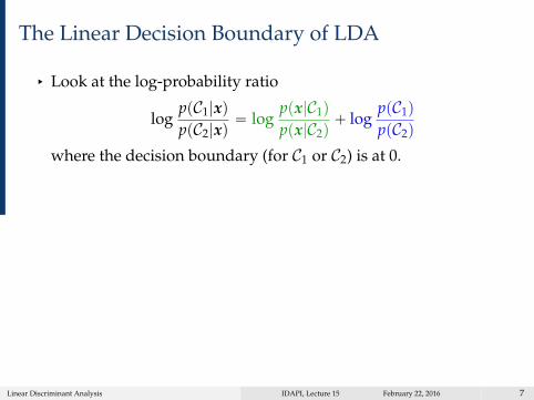
§ Look at the log-probability ratio
logppC1|xqppC2|xq
“ logppx|C1q
ppx|C2q` log
ppC1q
ppC2q
where the decision boundary (for C1 or C2) is at 0.
§ Assume Gaussian likelihood ppx|Ciq “ N`
x |mi, Σ˘
with thesame covariance in both classes. Decision boundary:
logppC1|xqppC2|xq
“ 0
ô logppC1q
ppC2q´
12pmJ
1 Σ´1m1 ´m2Σ´1m2q ` pm1 ´m2qJΣ´1x “ 0
ô pm1 ´m2qJΣ´1x “
12pmJ
1 Σ´1m1 ´m2Σ´1m2q ´ logppC1q
ppC2q
Of the form Ax “ b Decision boundary linear in x
Linear Discriminant Analysis IDAPI, Lecture 15 February 22, 2016 7

The Linear Decision Boundary of LDA
§ Look at the log-probability ratio
logppC1|xqppC2|xq
“ logppx|C1q
ppx|C2q` log
ppC1q
ppC2q
where the decision boundary (for C1 or C2) is at 0.§ Assume Gaussian likelihood ppx|Ciq “ N
`
x |mi, Σ˘
with thesame covariance in both classes. Decision boundary:
logppC1|xqppC2|xq
“ 0
ô logppC1q
ppC2q´
12pmJ
1 Σ´1m1 ´m2Σ´1m2q ` pm1 ´m2qJΣ´1x “ 0
ô pm1 ´m2qJΣ´1x “
12pmJ
1 Σ´1m1 ´m2Σ´1m2q ´ logppC1q
ppC2q
Of the form Ax “ b Decision boundary linear in xLinear Discriminant Analysis IDAPI, Lecture 15 February 22, 2016 7

Potential Issues
−2 2 6
−2
0
2
4
From PRML (Bishop, 2006)
§ Considerable loss of information when projecting
§ Even if data was linearly separable in RD, we may lose thisseparability (see figure)
Find good basis vector w that spans the subspace we project onto
Linear Discriminant Analysis IDAPI, Lecture 15 February 22, 2016 8

Potential Issues
−2 2 6
−2
0
2
4
From PRML (Bishop, 2006)
§ Considerable loss of information when projecting§ Even if data was linearly separable in RD, we may lose this
separability (see figure)
Find good basis vector w that spans the subspace we project onto
Linear Discriminant Analysis IDAPI, Lecture 15 February 22, 2016 8

Potential Issues
−2 2 6
−2
0
2
4
From PRML (Bishop, 2006)
§ Considerable loss of information when projecting§ Even if data was linearly separable in RD, we may lose this
separability (see figure)Find good basis vector w that spans the subspace we project onto
Linear Discriminant Analysis IDAPI, Lecture 15 February 22, 2016 8

Approach: Maximize Class Separation
§ Adjust components of basis vector wSelect projection that maximizes the class separation
§ Consider two classes: C1 with N1 points and C2 with N2 points
§ Corresponding mean vectors:
m1 “1
N1
ÿ
nPC1
xn , m2 “1
N2
ÿ
nPC2
xn
§ Measure class separation as the distance of the projected classmeans:
m2 ´m1 “ wJm2 ´wJm1 “ wJpm2 ´m1q
and maximize this w.r.t. w with the constraint }w} “ 1
Linear Discriminant Analysis IDAPI, Lecture 15 February 22, 2016 9

Maximum Class Separation
−2 2 6
−2
0
2
4
Larger distance between the means
Betterclassseparab
ility
From PRML (Bishop, 2006)
§ Find w 9 pm2 ´m1q
§ Projected classes may still have considerable overlap (because ofstrongly non-diagonal covariances of the class distributions)
§ LDA: Large separation of projected class means and smallwithin-class variation (small overlap of classes)
Linear Discriminant Analysis IDAPI, Lecture 15 February 22, 2016 10

Key Idea of LDA
−2 2 6
−2
0
2
4
From PRML (Bishop, 2006)
§ Separate samples of distinct groups by projecting them onto aspace that
§ Maximizes their between-class separability while§ Minimizing their within-class variability
Linear Discriminant Analysis IDAPI, Lecture 15 February 22, 2016 11

Fisher Criterion
§ For each class Ck the within-class scatter (unnormalized variance)is given as
s2k “
ÿ
nPCk
pyn ´mkq2 , yn “ wJxn , mk “ wJmk
§ Maximize the Fisher criterion:
Jpwq “Between-class scatterWithin-class scatter
“pm2 ´m1q
2
s21 ` s2
2“
wJSBwwJSWw
SW “ÿ
k
ÿ
nPCkpxn ´mkqpxn ´mkq
J
SB “ pm2 ´m1qpm2 ´m1qJ
§ SW is the total within-class scatter and proportional to the samplecovariance matrix
Linear Discriminant Analysis IDAPI, Lecture 15 February 22, 2016 12

Generalization to k Classes
For k classes, we define the between-class scatter matrix as
SB “ÿ
kNkpmk ´ µqpm2 ´ µqJ , µ “
1N
Nÿ
i“1
xi
where µ is the global mean of the data set
Linear Discriminant Analysis IDAPI, Lecture 15 February 22, 2016 13

Finding the Projection
ObjectiveFind w˚ that maximizes
Jpwq “wJSBwwJSWw
We find w by setting dJ{dw “ 0:
dJ{dw “ 0 ô`
wJSWw˘
SBw´`
wJSBw˘
SWw “ 0
ô SBw´ JSWw “ 0
ô S´1W SBw´ Jw “ 0
Eigenvalue problem S´1W SBw “ Jw
The projection vector w is the eigenvector of S´1W SB.
Choose the eigenvector that corresponds to the maximumeigenvalue (similar to PCA) to maximize class separability
Linear Discriminant Analysis IDAPI, Lecture 15 February 22, 2016 14

Finding the Projection
ObjectiveFind w˚ that maximizes
Jpwq “wJSBwwJSWw
We find w by setting dJ{dw “ 0:
dJ{dw “ 0 ô`
wJSWw˘
SBw´`
wJSBw˘
SWw “ 0ô SBw´ JSWw “ 0
ô S´1W SBw´ Jw “ 0
Eigenvalue problem S´1W SBw “ Jw
The projection vector w is the eigenvector of S´1W SB.
Choose the eigenvector that corresponds to the maximumeigenvalue (similar to PCA) to maximize class separability
Linear Discriminant Analysis IDAPI, Lecture 15 February 22, 2016 14

Algorithm
1. Mean normalization
2. Compute mean vectors mi P RD for all k classes
3. Compute scatter matrices SW , SB
4. Compute eigenvectors and eigenvalues of S´1W SB
5. Select k eigenvectors wi with the largest eigenvalues to form aDˆ k-dimensional matrix W “ rw1, . . . , wks
6. Project samples onto the new subspace using W and compute thenew coordinates as Y “ XW
§ X P RnˆD: ith row represents the ith sample
§ Y P Rnˆk: Coordinate matrix of the n data points w.r.t. eigenbasisW spanning the k-dimensional subspace
Linear Discriminant Analysis IDAPI, Lecture 15 February 22, 2016 15

PCA vs LDA
4 3 2 1 0 1 2 3 4 5PC1
4
3
2
1
0
1
2
3
4PC
2PCA: Iris projection onto the first 2 principal axes
setosaversicolorvirginica
1.5 1.0 0.5 0.0 0.5 1.0 1.5LD1
2.0
1.5
1.0
0.5
0.0
0.5
1.0
1.5
2.0
2.5
LD2
LDA: Iris projection onto the first 2 linear discriminants
setosaversicolorvirginica
§ Similar to PCA, we can use LDA for dimensionality reduction bylooking at an eigenvalue problem
§ LDA: Magnitude of the eigenvalues in LDA describe importanceof the corresponding eigenspace with respect to classificationperformance
§ PCA: Magnitude of the eigenvalues in LDA describe importanceof the corresponding eigenspace with respect to minimizingreconstruction error
Linear Discriminant Analysis IDAPI, Lecture 15 February 22, 2016 16

Assumptions in LDA
§ The true covariance matrices of each class are equal
§ Without this assumption: Quadratic discriminant analysis (e.g.Hastie et al., 2009)
§ Performance of the standard LDA can be seriously degraded ifthere are only a limited number of total training observations Ncompared to the dimension D of the feature space.
Shrinkage (Copas, 1983)
§ LDA explicitly attempts to model the difference between theclasses of data. PCA on the other hand does not take into accountany difference in class
Linear Discriminant Analysis IDAPI, Lecture 15 February 22, 2016 17

Limitations of LDA
§ LDA’s most disriminant features are the means of the datadistributions
§ LDA will fail when the discriminatory information is not themean but the variance of the data.
§ If the data distributions are very non-Gaussian, the LDAprojections will not preserve the complex structure of the datathat may be required for classification
Nonlinear LDA (e.g., Mika et al., 1999; Baudat & Anouar, 2000)Linear Discriminant Analysis IDAPI, Lecture 15 February 22, 2016 18

References I
[1] G. Baudat and F. Anouar. Generalized Discriminant Analysisusing a Kernel Approach. Neural Computation, 12(10):2385–2404,2000.
[2] C. M. Bishop. Pattern Recognition and Machine Learning.Information Science and Statistics. Springer-Verlag, 2006.
[3] J. B. Copas. Regression, Prediction and Shrinkage. Journal of theRoyal Statistical Society, Series B, 45(3):311–354, 1983.
[4] T. Hastie, R. Tibshirani, and J. Friedman. The Elements of StatisticalLearning—Data Mining, Inference, and Prediction. Springer Series inStatistics. Springer-Verlag New York, Inc., 175 Fifth Avenue, NewYork City, NY, USA, 2001.
[5] S. Mika, G. Ratsch, J. Weston, B. Scholkopf, and K.-R. Muller.Fisher Discriminant Analysis with Kernels. Neural Networks forSignal Processing, IX:41–48, 1999.
Linear Discriminant Analysis IDAPI, Lecture 15 February 22, 2016 19
Related Documents