Lecture 13 Dynamic analysis of feedback - …boyd/ee102/ctrl-dyn.pdf · Lecture 13 Dynamic analysis of feedback ... Feedback system: frequency domain ... Dynamic analysis of feedback

S. Boyd EE102

Lecture 13Dynamic analysis of feedback

• Closed-loop, sensitivity, and loop transfer functions

• Stability of feedback systems

13–1

Some assumptions

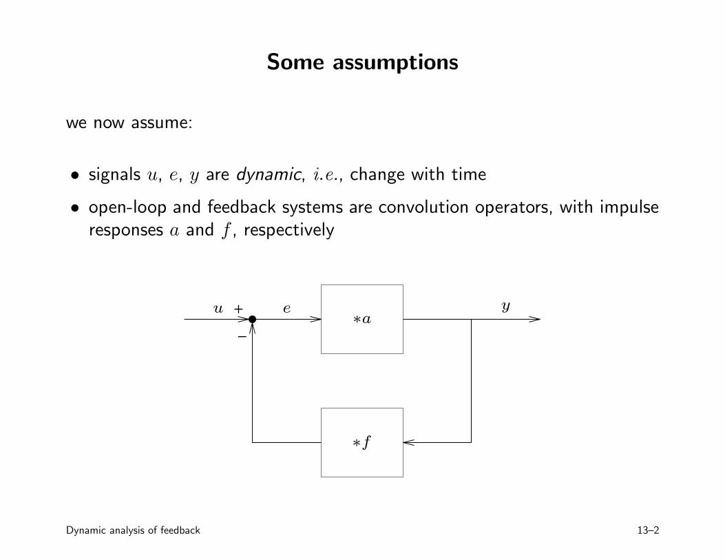
we now assume:

• signals u, e, y are dynamic, i.e., change with time

• open-loop and feedback systems are convolution operators, with impulseresponses a and f , respectively

PSfrag replacements

u ye∗a

∗f

Dynamic analysis of feedback 13–2

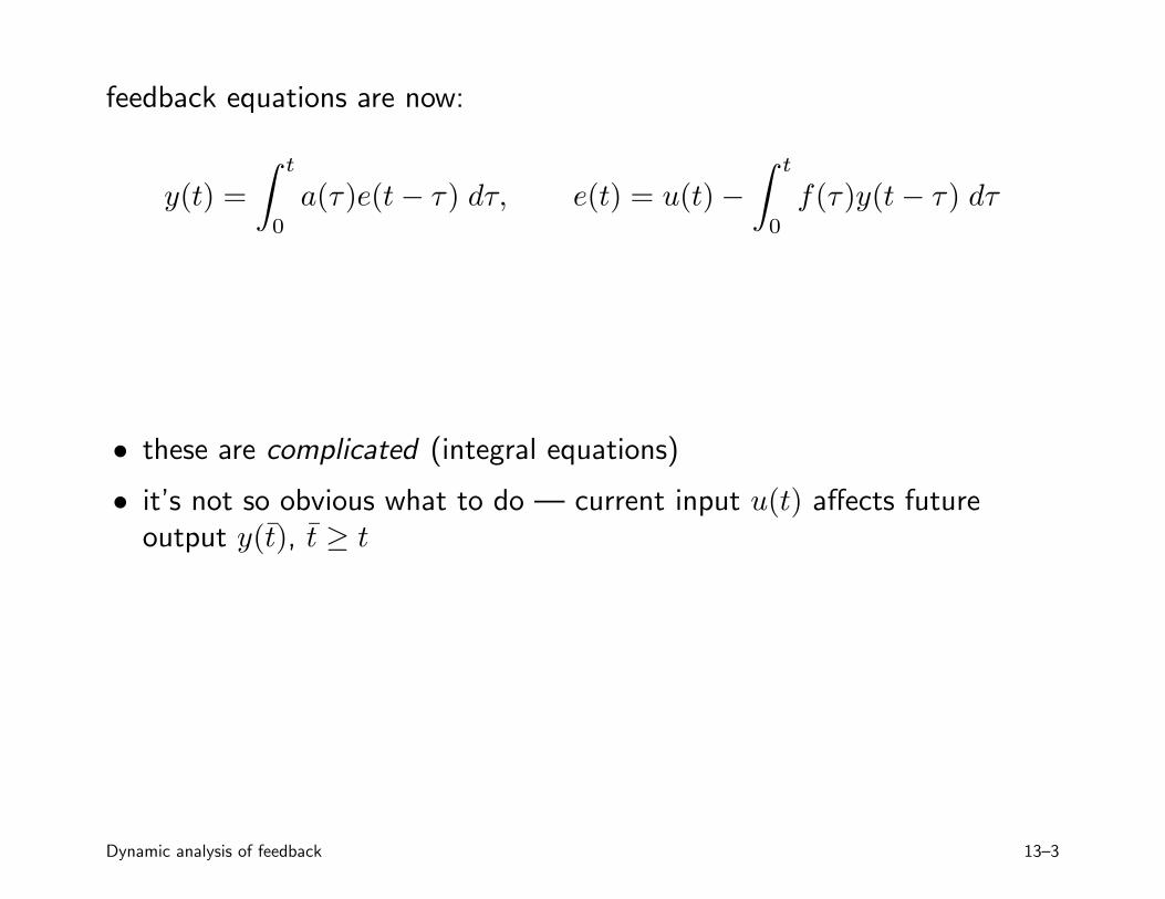
feedback equations are now:

y(t) =

∫ t

0

a(τ)e(t− τ) dτ, e(t) = u(t)−

∫ t

0

f(τ)y(t− τ) dτ

• these are complicated (integral equations)

• it’s not so obvious what to do — current input u(t) affects futureoutput y(t̄), t̄ ≥ t


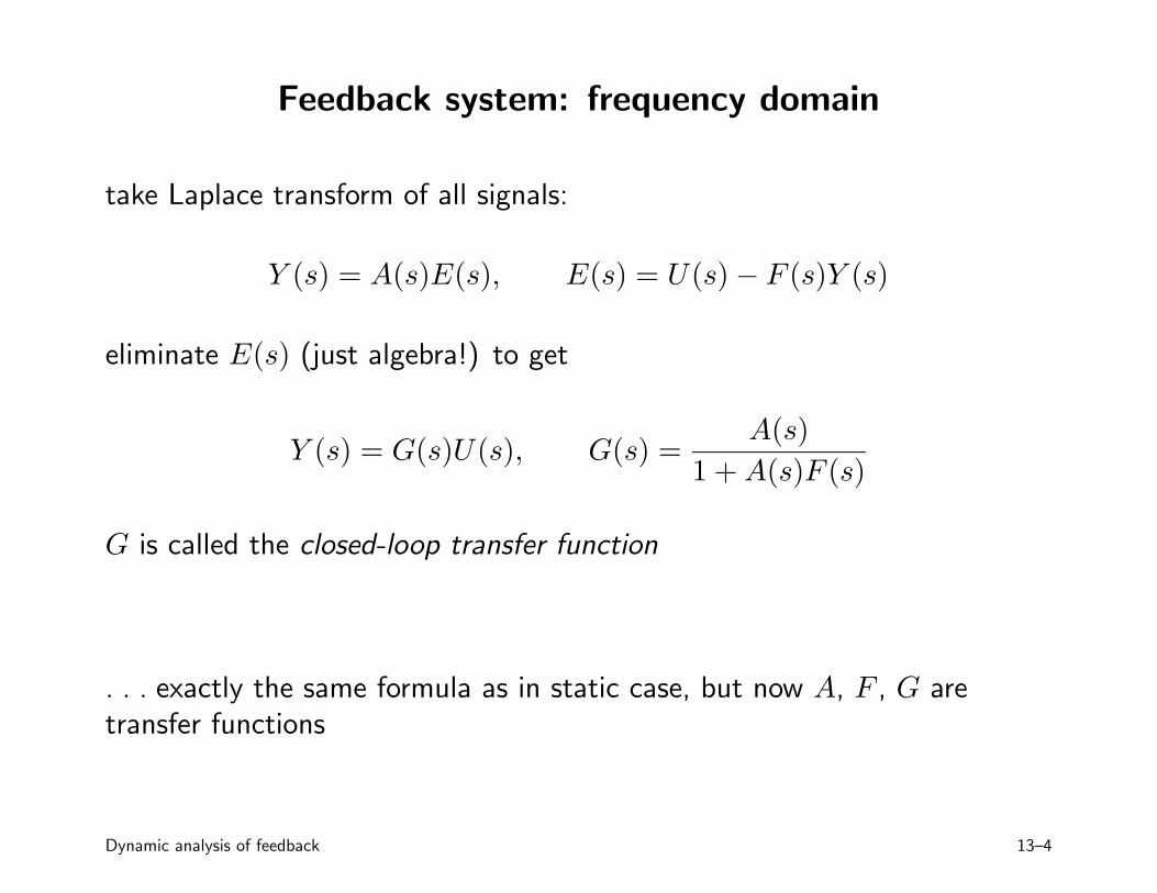
Feedback system: frequency domain

take Laplace transform of all signals:

Y (s) = A(s)E(s), E(s) = U(s)− F (s)Y (s)

eliminate E(s) (just algebra!) to get

Y (s) = G(s)U(s), G(s) =A(s)

1 +A(s)F (s)

G is called the closed-loop transfer function

. . . exactly the same formula as in static case, but now A, F , G aretransfer functions


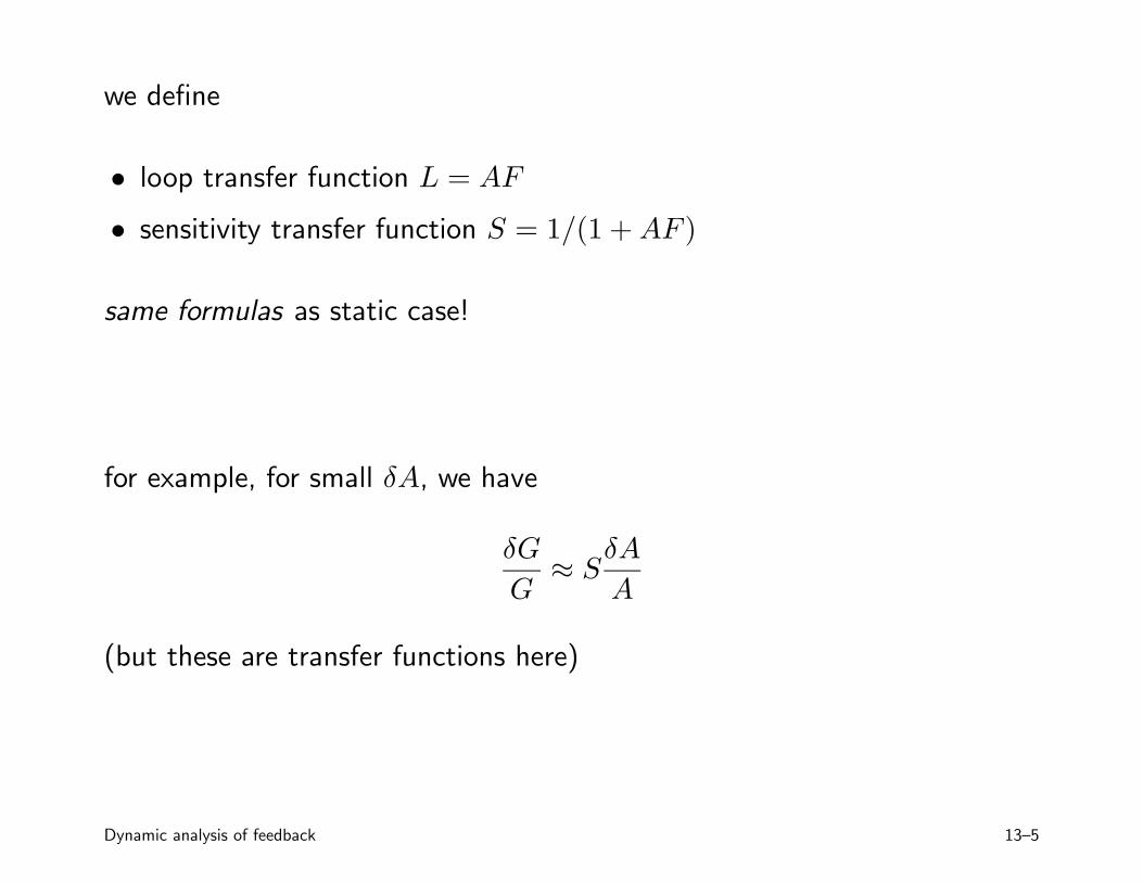
we define

• loop transfer function L = AF

• sensitivity transfer function S = 1/(1 +AF )

same formulas as static case!

for example, for small δA, we have

δG

G≈ S

δA

A

(but these are transfer functions here)


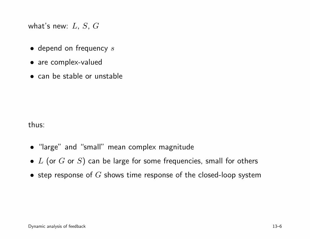
what’s new: L, S, G

• depend on frequency s

• are complex-valued

• can be stable or unstable

thus:

• “large” and “small” mean complex magnitude

• L (or G or S) can be large for some frequencies, small for others

• step response of G shows time response of the closed-loop system


Example

feedback system with

A(s) =105

1 + s/100, F = 0.01

• open-loop gain is large at DC (105)

• open-loop bandwidth is around 100 rad/sec

• open-loop settling time is around 20msec


closed-loop transfer function is

G(s) =

105

1+s/100

1 + 0.01 105

1+s/100

=99.9

1 + s/(1.001·105)

• G is stable

• closed-loop DC gain is very nearly 1/F

• closed-loop bandwidth around 105 rad/sec

• closed-loop settling time is around 20µsec

. . . closed-loop system has lower gain, higher bandwidth, i.e., is faster


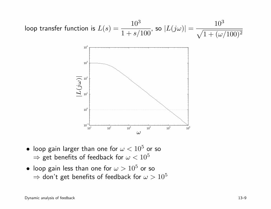
loop transfer function is L(s) =103

1 + s/100, so |L(jω)| =

103

√

1 + (ω/100)2

101

102

103

104

105

106

10−1

100

101

102

103

104

PSfrag replacements

|L(jω)|

ω

• loop gain larger than one for ω < 105 or so⇒ get benefits of feedback for ω < 105

• loop gain less than one for ω > 105 or so⇒ don’t get benefits of feedback for ω > 105


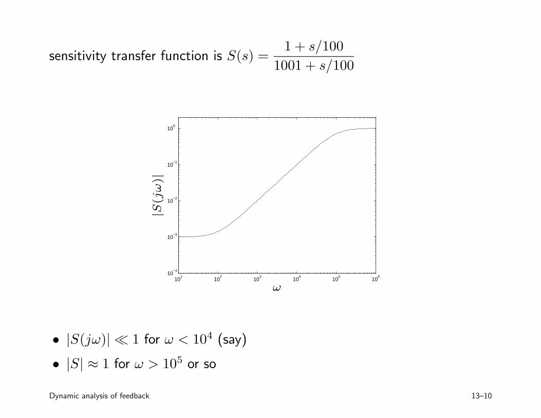
sensitivity transfer function is S(s) =1 + s/100

1001 + s/100

101

102

103

104

105

106

10−4

10−3

10−2

10−1

100

PSfrag replacements

|S(jω)|

ω

• |S(jω)| ¿ 1 for ω < 104 (say)

• |S| ≈ 1 for ω > 105 or so


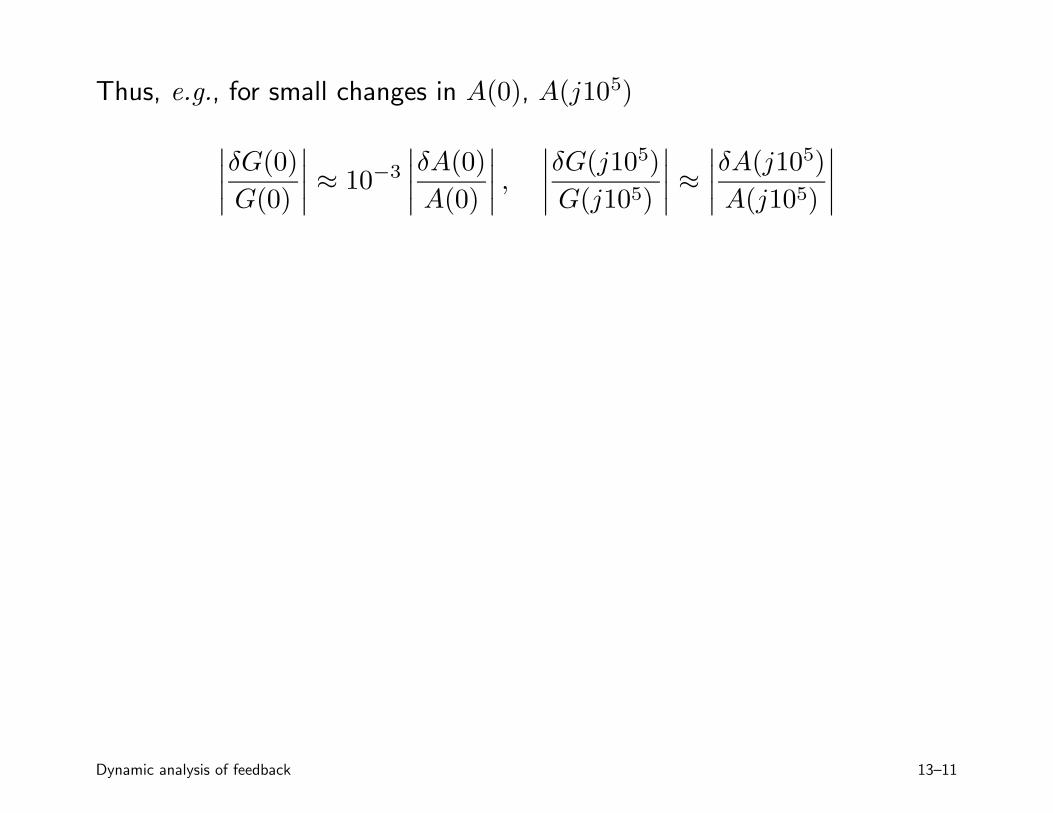
Thus, e.g., for small changes in A(0), A(j105)

∣

∣

∣

∣

δG(0)

G(0)

∣

∣

∣

∣

≈ 10−3

∣

∣

∣

∣

δA(0)

A(0)

∣

∣

∣

∣

,

∣

∣

∣

∣

δG(j105)

G(j105)

∣

∣

∣

∣

≈

∣

∣

∣

∣

δA(j105)

A(j105)

∣

∣

∣

∣


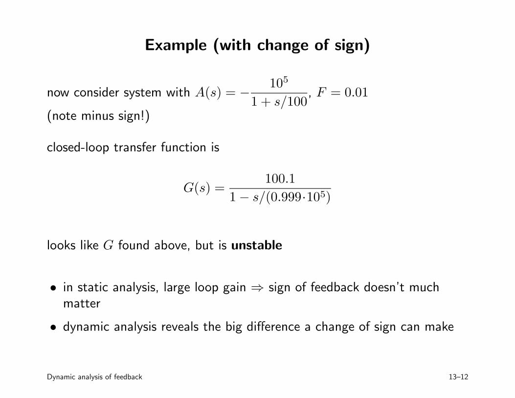
Example (with change of sign)

now consider system with A(s) = −105

1 + s/100, F = 0.01

(note minus sign!)

closed-loop transfer function is

G(s) =100.1

1− s/(0.999·105)

looks like G found above, but is unstable

• in static analysis, large loop gain ⇒ sign of feedback doesn’t muchmatter

• dynamic analysis reveals the big difference a change of sign can make


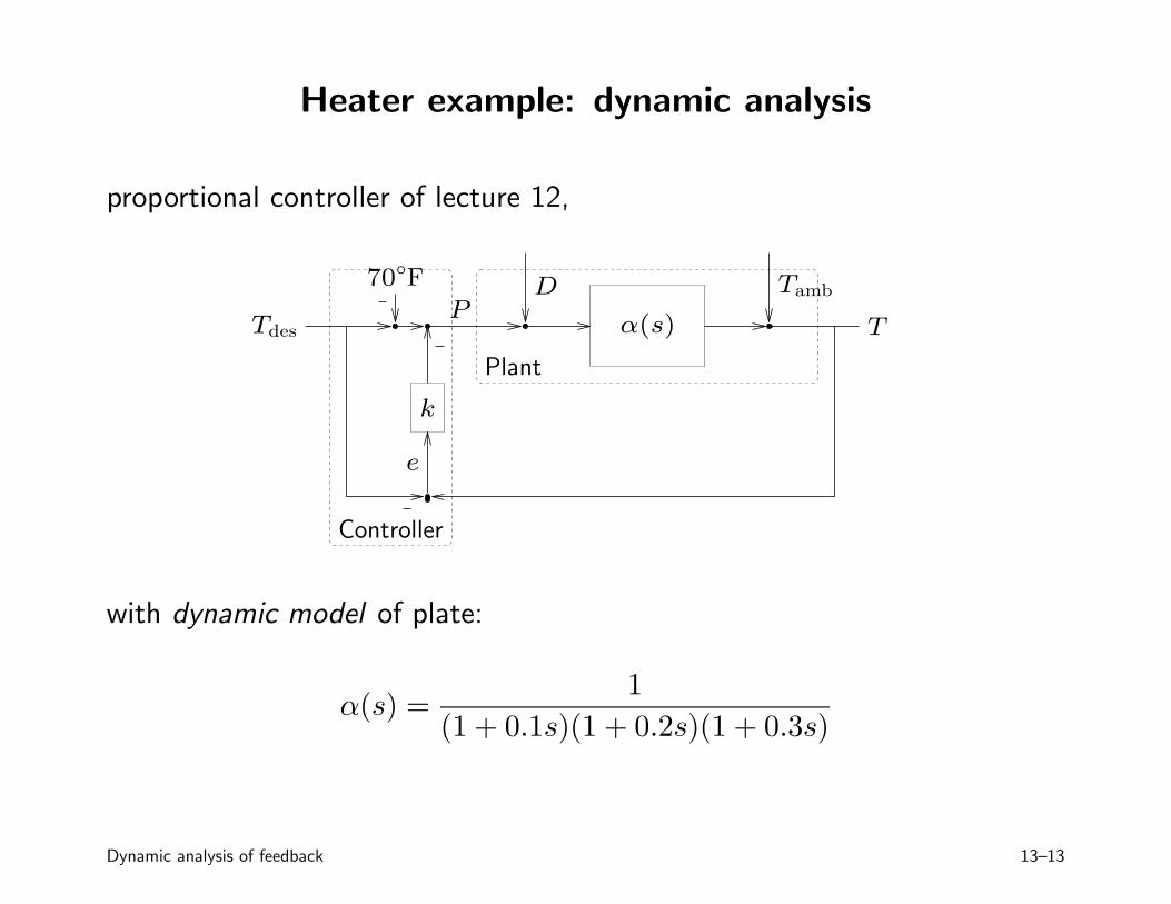
Heater example: dynamic analysis

proportional controller of lecture 12,PSfrag replacements

P

70◦F D

α(s) T

Tamb

Tdes

e

k

Plant

Controller

with dynamic model of plate:

α(s) =1

(1 + 0.1s)(1 + 0.2s)(1 + 0.3s)


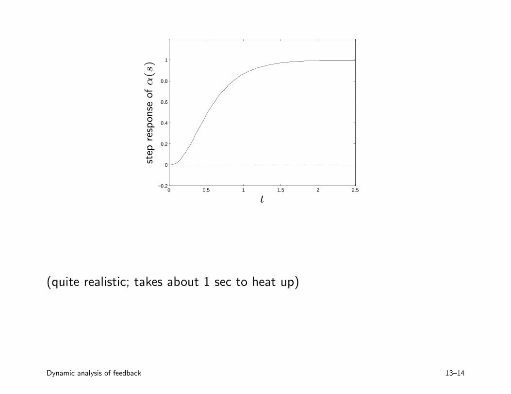
0 0.5 1 1.5 2 2.5−0.2

0

0.2

0.4

0.6

0.8

1

PSfrag replacements

t

step

resp

onse

ofα(s

)

(quite realistic; takes about 1 sec to heat up)


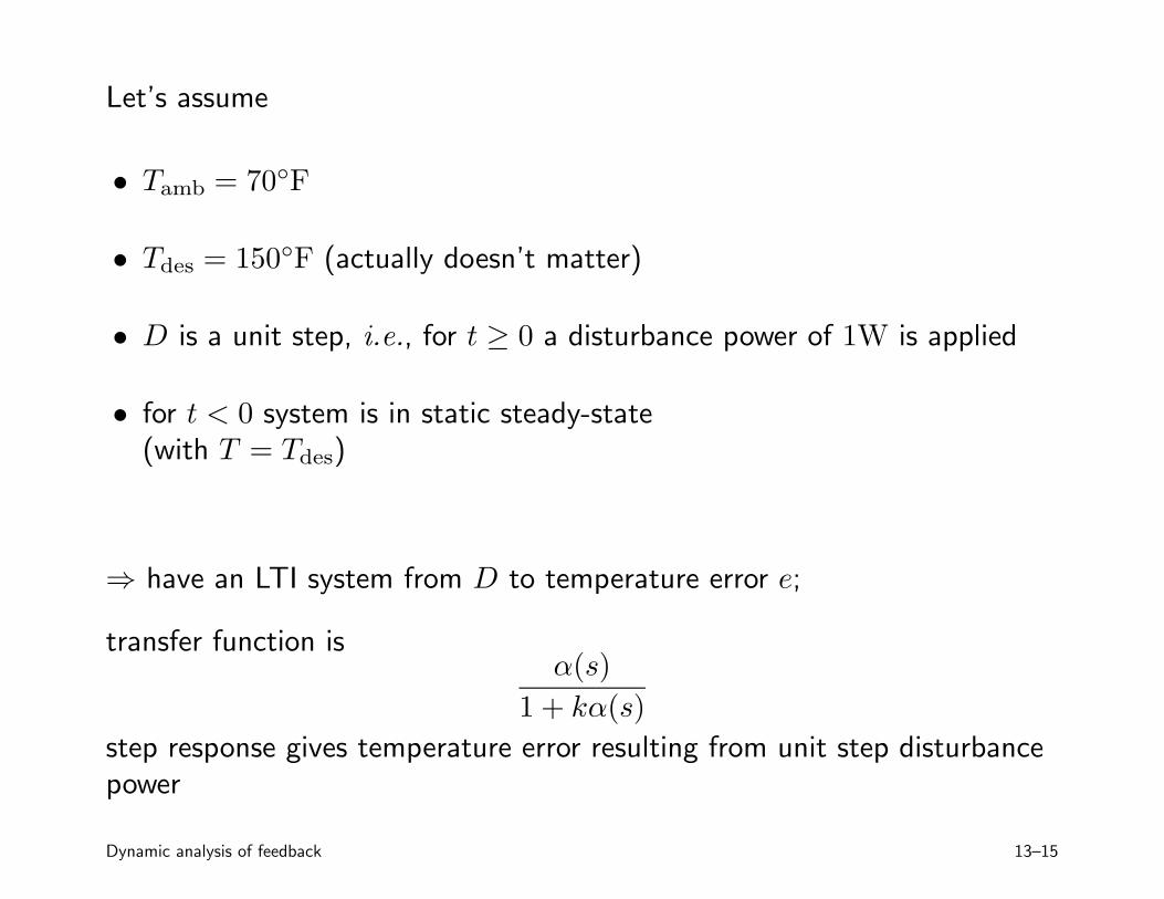
Let’s assume

• Tamb = 70◦F

• Tdes = 150◦F (actually doesn’t matter)

• D is a unit step, i.e., for t ≥ 0 a disturbance power of 1W is applied

• for t < 0 system is in static steady-state(with T = Tdes)

⇒ have an LTI system from D to temperature error e;

transfer function isα(s)

1 + kα(s)

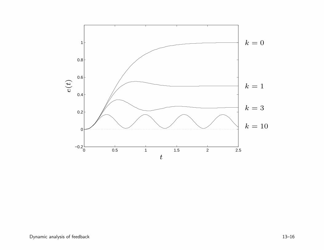
step response gives temperature error resulting from unit step disturbancepower


0 0.5 1 1.5 2 2.5−0.2

0

0.2

0.4

0.6

0.8

1

PSfrag replacements

t

e(t

)

k = 0

k = 1

k = 3

k = 10


0 0.5 1 1.5 2 2.5 3 3.5 4 4.5 5−3

−2

−1

0

1

2

3

PSfrag replacements

t

e(t

)k = 0

k = 12

k = 15


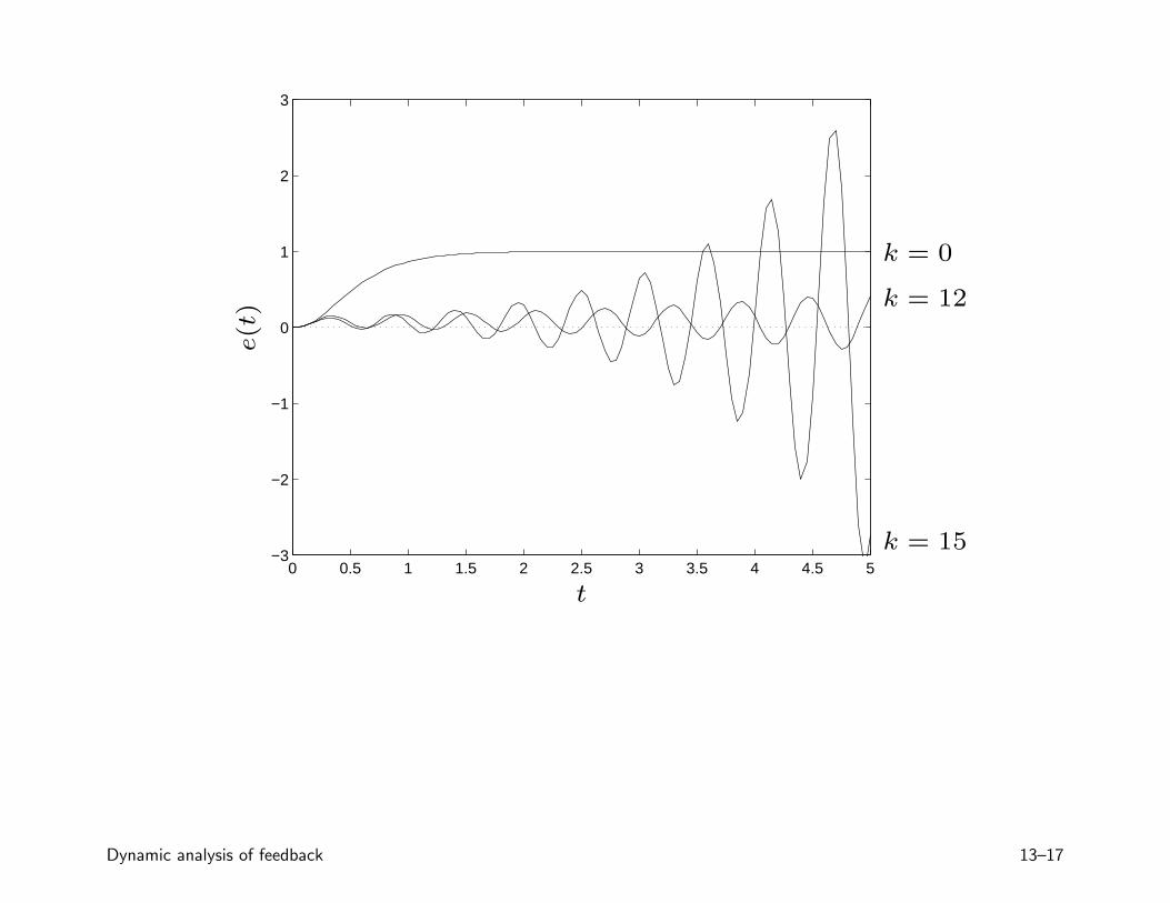
• closed-loop system can exhibit oscillatory response

• for k < 10 (approximately) this transfer function is stable; for k > 10(approximately) it is unstable

• when stable, step response settles to DC gain, 1/(1 + k)

• stability requirement limits how large proportional gain (hence loopgain) can be

these are general phenomena


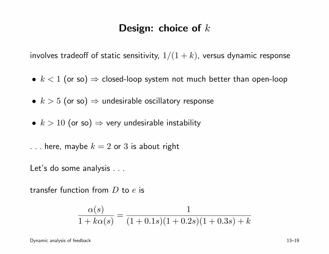
Design: choice of k

involves tradeoff of static sensitivity, 1/(1 + k), versus dynamic response

• k < 1 (or so) ⇒ closed-loop system not much better than open-loop

• k > 5 (or so) ⇒ undesirable oscillatory response

• k > 10 (or so) ⇒ very undesirable instability

. . . here, maybe k = 2 or 3 is about right

Let’s do some analysis . . .

transfer function from D to e is

α(s)

1 + kα(s)=

1

(1 + 0.1s)(1 + 0.2s)(1 + 0.3s) + k


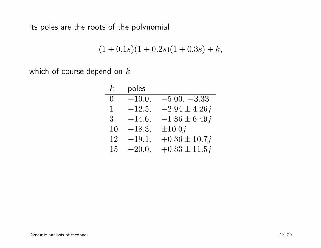
its poles are the roots of the polynomial

(1 + 0.1s)(1 + 0.2s)(1 + 0.3s) + k,

which of course depend on k

k poles0 −10.0, −5.00, −3.331 −12.5, −2.94± 4.26j3 −14.6, −1.86± 6.49j10 −18.3, ±10.0j12 −19.1, +0.36± 10.7j15 −20.0, +0.83± 11.5j


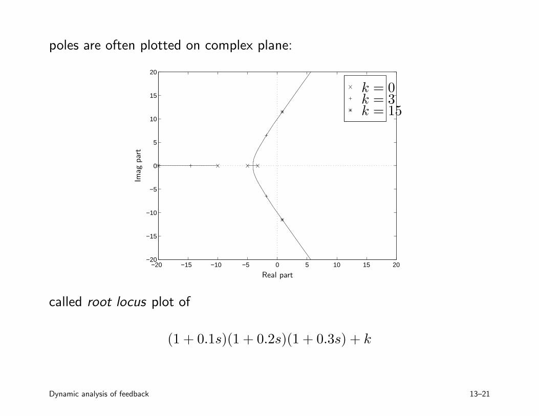
poles are often plotted on complex plane:

−20 −15 −10 −5 0 5 10 15 20−20

−15

−10

−5

0

5

10

15

20

PSfrag replacements

Real part

Imag

par

t

k = 0k = 3k = 15

called root locus plot of

(1 + 0.1s)(1 + 0.2s)(1 + 0.3s) + k


Checking stability

when is H(s) = b(s)/a(s) stable?

i.e., when do all roots of the polynomial a have negative real parts(such polynomials are called Hurwitz)

if a is already factored, as in

a(s) = α(s− p1)(s− p2) · · · (s− pn),

we just check <(pi) < 0 for i = 1, . . . , n

what if we are given the coefficients of a:

a(s) = a0 + a1s+ a2s2 + · · ·+ ans

n


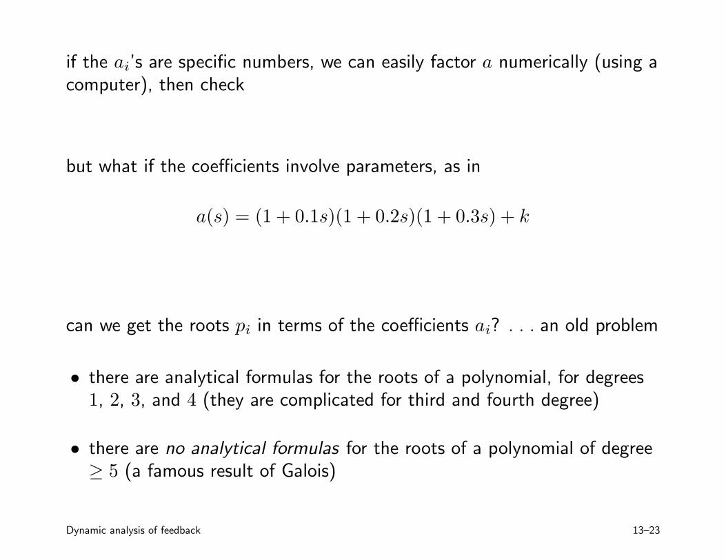
if the ai’s are specific numbers, we can easily factor a numerically (using acomputer), then check

but what if the coefficients involve parameters, as in

a(s) = (1 + 0.1s)(1 + 0.2s)(1 + 0.3s) + k

can we get the roots pi in terms of the coefficients ai? . . . an old problem

• there are analytical formulas for the roots of a polynomial, for degrees1, 2, 3, and 4 (they are complicated for third and fourth degree)

• there are no analytical formulas for the roots of a polynomial of degree≥ 5 (a famous result of Galois)


still, it turns out that we can express the Hurwitz condition as a set ofalgebraic inequalities involving the coefficients, using Routh’s method(1870 or so)

• very useful 50 years ago, even for polynomials with specific numericcoefficients

• only important nowadays for polynomials with parameters


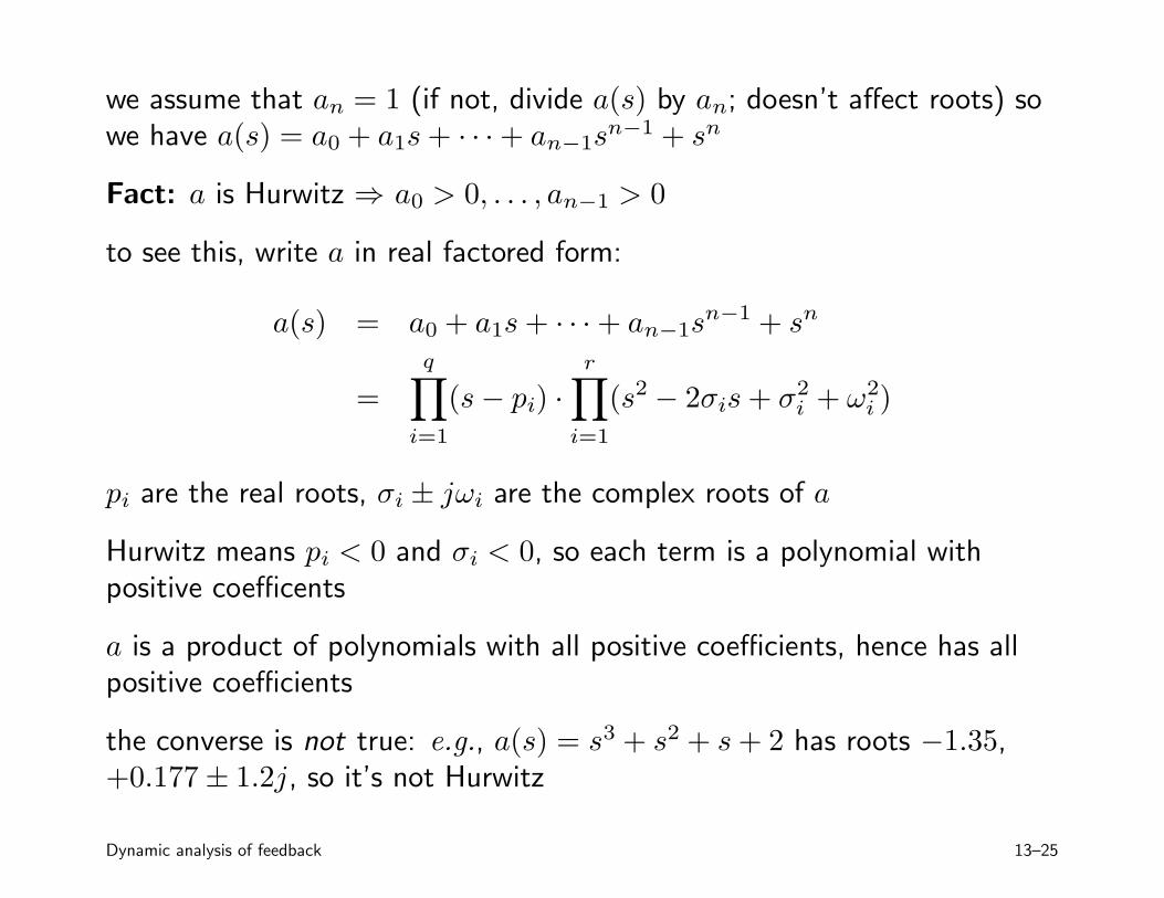
we assume that an = 1 (if not, divide a(s) by an; doesn’t affect roots) sowe have a(s) = a0 + a1s+ · · ·+ an−1s

n−1 + sn

Fact: a is Hurwitz ⇒ a0 > 0, . . . , an−1 > 0

to see this, write a in real factored form:

a(s) = a0 + a1s+ · · ·+ an−1sn−1 + sn

=

q∏

i=1

(s− pi) ·

r∏

i=1

(s2 − 2σis+ σ2i + ω2

i )

pi are the real roots, σi ± jωi are the complex roots of a

Hurwitz means pi < 0 and σi < 0, so each term is a polynomial withpositive coefficents

a is a product of polynomials with all positive coefficients, hence has allpositive coefficients

the converse is not true: e.g., a(s) = s3 + s2 + s+ 2 has roots −1.35,+0.177± 1.2j, so it’s not Hurwitz


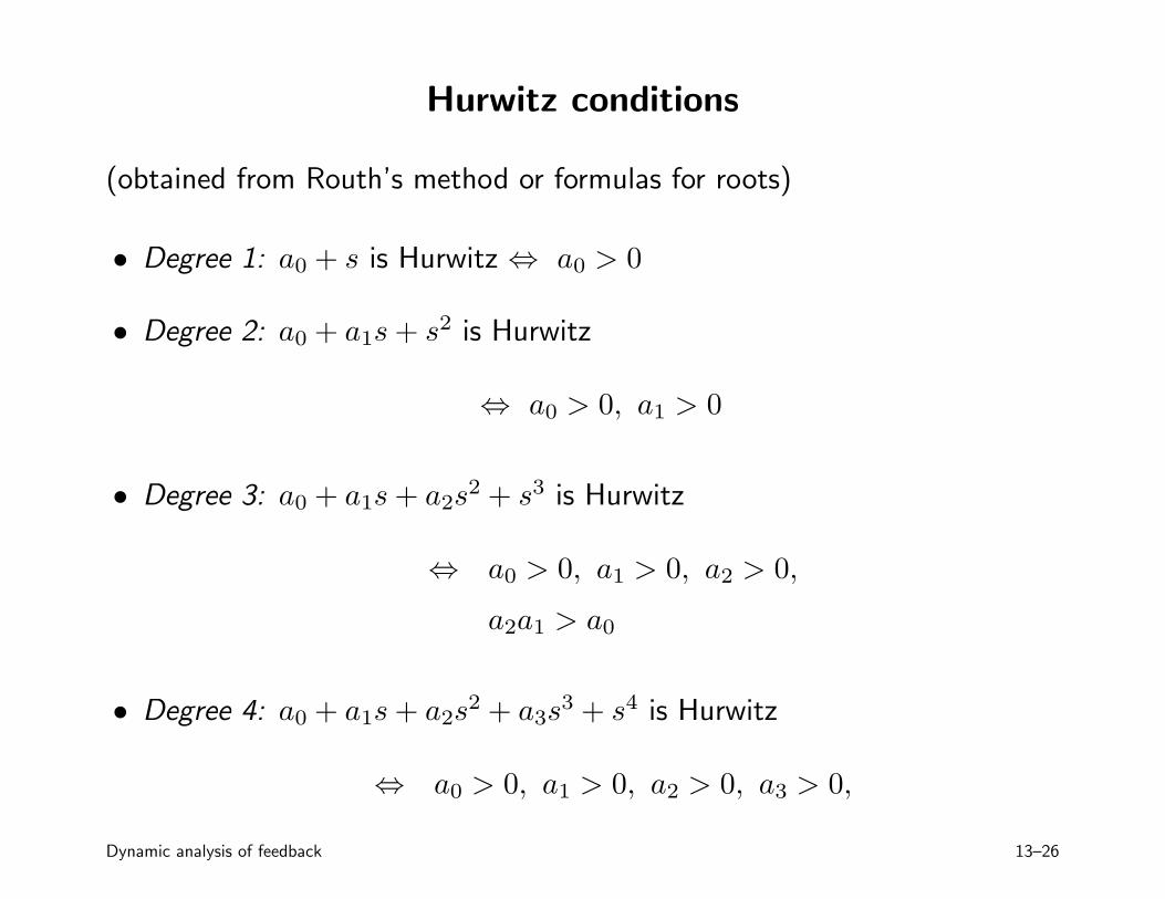
Hurwitz conditions

(obtained from Routh’s method or formulas for roots)

• Degree 1: a0 + s is Hurwitz ⇔ a0 > 0

• Degree 2: a0 + a1s+ s2 is Hurwitz

⇔ a0 > 0, a1 > 0

• Degree 3: a0 + a1s+ a2s2 + s3 is Hurwitz

⇔ a0 > 0, a1 > 0, a2 > 0,

a2a1 > a0

• Degree 4: a0 + a1s+ a2s2 + a3s

3 + s4 is Hurwitz

⇔ a0 > 0, a1 > 0, a2 > 0, a3 > 0,


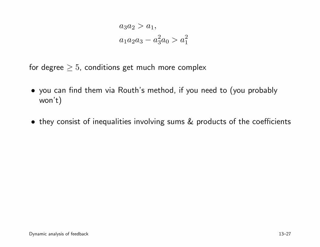
a3a2 > a1,

a1a2a3 − a23a0 > a2

1

for degree ≥ 5, conditions get much more complex

• you can find them via Routh’s method, if you need to (you probablywon’t)

• they consist of inequalities involving sums & products of the coefficients


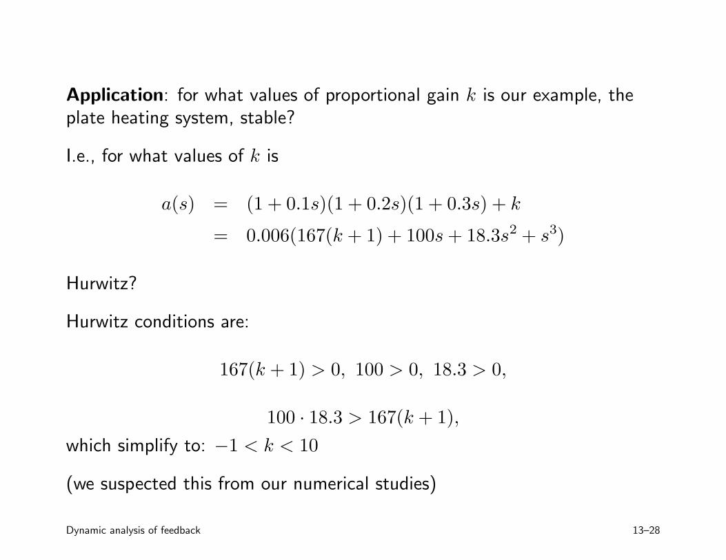
Application: for what values of proportional gain k is our example, theplate heating system, stable?

I.e., for what values of k is

a(s) = (1 + 0.1s)(1 + 0.2s)(1 + 0.3s) + k

= 0.006(167(k + 1) + 100s+ 18.3s2 + s3)

Hurwitz?

Hurwitz conditions are:

167(k + 1) > 0, 100 > 0, 18.3 > 0,

100 · 18.3 > 167(k + 1),

which simplify to: −1 < k < 10

(we suspected this from our numerical studies)


Summary

for LTI feedback systems,

• formulas same as static case, but now A, F , L, S are transfer functions

• hence are complex, depend on frequency s, and can be stable orunstable

• stability requirement often limits the amount of feedback that can beused


Lecture 13 Dynamic analysis of feedback - …boyd/ee102/ctrl-dyn.pdf · Lecture 13 Dynamic analysis of feedback ... Feedback system: frequency domain ... Dynamic analysis of feedback

Documents