Lecture 12 -- Windowing and grid techniques - Home | EM …emlab.utep.edu/ee5390fdtd/Lecture 12 -- Windowing and grid...Lecture Outline Lecture 12 Slide 2 ... HH H HDD zxct HH ...

9/26/2016

1

Lecture 12 Slide 1

EE 5303

Electromagnetic Analysis Using Finite‐Difference Time‐Domain

Lecture #12

Windowing and Grid Techniques These notes may contain copyrighted material obtained under fair use rules.  Distribution of these materials is strictly prohibited  

Lecture Outline

Lecture 12 Slide 2

• Review of Lecture 11

• Windowing

• 2× Grid Technique

• Dielectric Averaging How to minimize the consequences of fitting devices to a Cartesian grid.

How to minimize the consequences of limiting the duration of the simulation.

How to construct the material arrays of arbitrarily shaped structures.

9/26/2016

2

Lecture 12 Slide 3

Review of Lecture 11

Lecture 12 Slide 4

Maxwell’s Equation with Normalized Electric Field

We normalized the quantities associated with the electric field

0

0 0

1E E E

Maxwell’s equations became

0

0 0

1D D c D

0

0

1

r

DH

c t

HE

c t

rD E

9/26/2016

3

Lecture 12 Slide 5

Revised Flow of Maxwell’s Equations

0

r HE

c t

Update H from E

Update D from H

0

1 DH

c t

Update E from D

rD E

time

x & y

x & y

x & y

Lecture 12 Slide 6

Expanded Maxwell’s Equations

These are the final form of Maxwell’s equations from which we will formulate the 2D and 3D FDTD method.

0

0

0

1

1

1

y xz

yx z

y x z

H DH

y z c t

DH H

z x c t

H H D

x y c t

0

0

0

y xx xz

yy yx z

y x zz z

E HE

y z c t

HE E

z x c t

E E H

x y c t

x xx x

y yy y

z zz z

D E

D E

D E

9/26/2016

4

Lecture 12 Slide 7

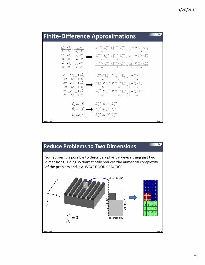
Finite‐Difference Approximations

0

0

0

y xx xz

yy yx z

y x zz z

E HE

y z c t

HE E

z x c t

E E H

x y c t

2 2

2 2

, 1, , , , , 1 , , , , , ,, ,

0

, , , ,, , 1 , , 1, , , , , ,

0

1, , , ,

t t

t t

i j k i j k i j k i j k i j k i j ki j kx xz z y y t txxt t t t

i j k i j ki j k i j k i j k i j k i j ky yx x z z t tyyt t t t

i j k i j k

y y xt t t

H HE E E E

y z c t

H HE E E E

z x c t

E E E

x

2 2

, 1, , , , , , ,, ,

0

t t

i j k i j k i j k i j ki j kz zx t tzzt

H HE

y c t

0

0

0

1

1

1

y xz

yx z

y x z

H DH

y z c t

DH H

z x c t

H H D

x y c t

2 2 2 2

2 2 2 2

2 2

, , , , 1 , , , ,, , , 1,

0

, , , ,, , , , 1 , , 1, ,

0

, , 1, ,

1

1

t t t t

t t t t

t t

i j k i j k i j k i j ki j k i j ky yz z x xt t t t t t t

i j k i j ki j k i j k i j k i j k

x x z z y yt t t t t t t

i j k i j

y yt t

H HH H D D

y z c t

H H H H D D

z x c t

H H

2 2

, , , ,, , , 1,

0

1t t

k i j k i j ki j k i j k

x x z zt t t t tH H D D

x y c t

x xx x

y yy y

z zz z

D E

D E

D E

, , , ,, ,

, , , ,, ,

, , , ,, ,

i j k i j ki j k

x xx xt t

i j k i j ki j k

y yy yt t

i j k i j ki j k

z zz zt t

D E

D E

D E

Lecture 12 Slide 8

Reduce Problems to Two Dimensions

Sometimes it is possible to describe a physical device using just two dimensions.  Doing so dramatically reduces the numerical complexity of the problem and is ALWAYS GOOD PRACTICE.

periodic BC

perio

dic B

C

absorbing BC

absorbing BC

z

x

y

0z

9/26/2016

5

Lecture 12 Slide 9

Two Distinct Modes

EzMode

z zz zD E , ,,i j i ji j

z zz zt tD E

yH xz

H HC

x y

E zx

E zy

EC

y

EC

x

0

0

E xx xx

yy yEy

HC

c t

HC

c t

0

1H zz

DC

c t

, 1 ,

,

1, ,

,

i j i j

i j z zE t tx t

i j i j

i j z zE t ty t

E EC

y

E EC

x

2 2

2 2

, ,,,

0

, ,,

,

0

t t

t t

i j i ji ji j x xt txxE

x t

i j i ji jy yi j t tyyE

y t

H HC

c t

H HC

c t

2 2 2 2

2

, 1, , , 1

, t t t t

t

i j i j i j i jy yi j x xt t t tH

z t

H H H HC

x y

2

, ,

,

0

1t

i j i j

i j z zH t t tz t

D DC

c t

HzMode

x xx x

y yy y

D E

D E

, ,,

, ,,

i j i ji j

x xx xt t

i j i ji j

y yy yt t

D E

D E

H zx

H zy

HC

y

HC

x

yE xz

E EC

x y

0

E zz zz

HC

c t

0

0

1

1

H xx

yHy

DC

c t

DC

c t

1, , , 1 ,

,

i j i j i j i j

i j y y x xE t t t tz t

E E E EC

x y

2 2

, ,,,

0

t t

i j i ji ji j z zt tzzE

z t

H HC

c t

2 2

2

2 2

2

, , 1

,

, 1,

,

t t

t

t t

t

i j i j

i j z zt tHx t

i j i j

i j z zt tHy t

H HC

y

H HC

x

2

2

, ,

,

0

, ,

,

0

1

1

t

t

i j i j

i j x xH t t tx t

i j i j

i j y yH t t ty t

D DC

c t

D DC

c t

Lecture 12 Slide 10

FDTD Algorithm for EzMode

, 1 , 1, ,

, ,

, ,

0 0

y

i j i j i j i jz z z zt t t t

y xi j i jE Ex yi N i jt t

z zt ty x

E E E Ej N i N

y xC CE E

j N i Ny x

2 2 2 2 2

, ,, ,, , 0 0, , t t t t t

i j i ji j i ji j i j E Ex x x y y yi j i jt t t tt t

xx yy

c t c tH H C H H C

2 2 2 2

2 2 2

2 2 2

, 1, , , 1

1, 1, 1, 1

,

,1 1,12 ,1

for 1 and 1

0 for 1 and 1

t t t t

t t t

t t t

i j i j i j i jy y x xt t t t

j j jy x xt t t

i jHz i it t i

y y xt t t

H H H Hi j

x y

H H Hi j

x yC

H H H

x

2 2

1,1 1,1

0 for 1 and 1

0 0 for 1 and 1

t ty xt t

i jy

H Hi j

x y

, , ,

0

i j i j i jHz z z tt t tD D c t C

, ,

,

1i j i j

z zi jt t t tzz

E D

time

src src src src, ,i j i j

z zt t t tD D g T

x & y

x & y

x & y

x & y

x & y

Simple soft source

9/26/2016

6

Lecture 12 Slide 11

Lecture 12 Slide 12

Time Response from FDTD

FDTD is a time‐domain method so it is the transient response of a device that is characterized.  A Fourier transform must be used to calculate frequency‐domain, or steady‐state, quantities.

source

reflected field transmitted field

9/26/2016

7

Lecture 12 Slide 13

Duration of the Simulation (i.e. STEPS)What happens when the simulation is stopped at time ts before the simulation is “finished?”

source

reflected field transmitted field

st st

st

Lecture 12 Slide 14

Example Impulse Response

FDTD produces the “impulse response” h(t) of a device.  In principle, the impulse response extends to infinity.

The spectrum of the infinite impulse response may be something like this…

h t

H

9/26/2016

8

Lecture 12 Slide 15

Mathematical Description of Finite Duration

When a simulation is stopped at time ts, it is just like multiplying the infinite impulse response by a pulse function w(t) with duration ts.

This is the resulting “infinite” impulse response when the simulation time is truncated.

h t w t

h t w t

Lecture 12 Slide 16

A Property of the Fourier Transform

The Fourier transform of the product of two functions is the convolution of the Fourier transform of the two functions.  

In terms of our functions h(t) and w(t), this is

F F Fh t ht t Htw w W

9/26/2016

9

Lecture 12 Slide 17

Fourier Transform of the Window Function

The window function and its Fourier transform are:

w t

W

Lecture 12 Slide 18

H() is “Blurred” by the Window Function

Every point H() is essentially blurred by the window function W() due to the convolution.

W

H

H W

9/26/2016

10

Lecture 12 Slide 19

Severity Trend for Windowing

• Long simulation time•Wide window• Narrow window spectrum• Less “blurring”• High frequency resolution

•Moderate simulation time•Moderate window•Moderate window spectrum•More “blurring”• Reduced frequency resolution

• Short simulation time• Narrow window•Wide window spectrum•Much “blurring”• Poor frequency resolution

W

H

h t

w t

H W

W

H

h t

w t

H W

W

H

h t

w t

H W

Lecture 12 Slide 20

Sampling and Windowing in FDTD

Given the time step t, the Nyquist sampling theorem quantifies the highest frequency that can be resolved.

max

1

2f

t

Given the FDTD simulation runs for STEPS number of iterations, the frequency resolution is

max2 1

STEPS STEPS

ff

t

Therefore, to resolve the frequency response down to a resolution of f, the number of iterations required is

1STEPS

t f

Note:  In practice, you should setmax

1 10t

t

t NN f

Notes:1. This is related to the uncertainty principle.2. You can calculate kernels for very finely spaced frequency 

points, but the actual frequency resolution is still limited by the windowing effect.  Your data will be “blurred.”

9/26/2016

11

Lecture 12 Slide 21

2× Grid Technique

Lecture 12 Slide 22

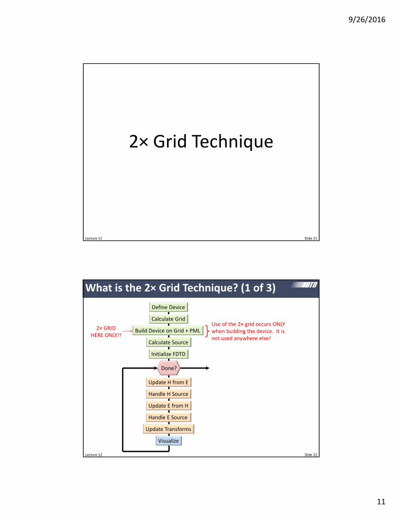
What is the 2× Grid Technique? (1 of 3)

Define Device

Calculate Grid

Build Device on Grid + PML

Calculate Source

Initialize FDTD

Update H from E

Handle H Source

Update E from H

Handle E Source

Update Transforms

Visualize

Done?

Use of the 2× grid occurs ONLY when building the device.  It is not used anywhere else!

2× GRIDHERE ONLY!!

9/26/2016

12

Lecture 12 Slide 23

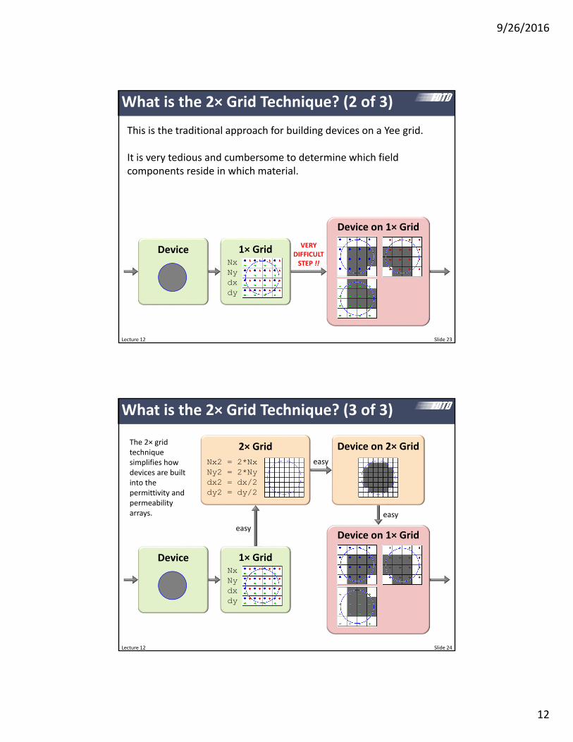
What is the 2× Grid Technique? (2 of 3)

DeviceNxNydxdy

1× Grid

Device on 1× Grid

VERY DIFFICULT STEP !!

This is the traditional approach for building devices on a Yee grid.  

It is very tedious and cumbersome to determine which field components reside in which material.

Lecture 12 Slide 24

What is the 2× Grid Technique? (3 of 3)

DeviceNxNydxdy

1× Grid

Device on 1× Grid

Nx2 = 2*NxNy2 = 2*Nydx2 = dx/2dy2 = dy/2

2× Grid Device on 2× Grid

easy

easy

easy

The 2× grid technique simplifies how devices are built into the permittivity and permeability arrays.

9/26/2016

13

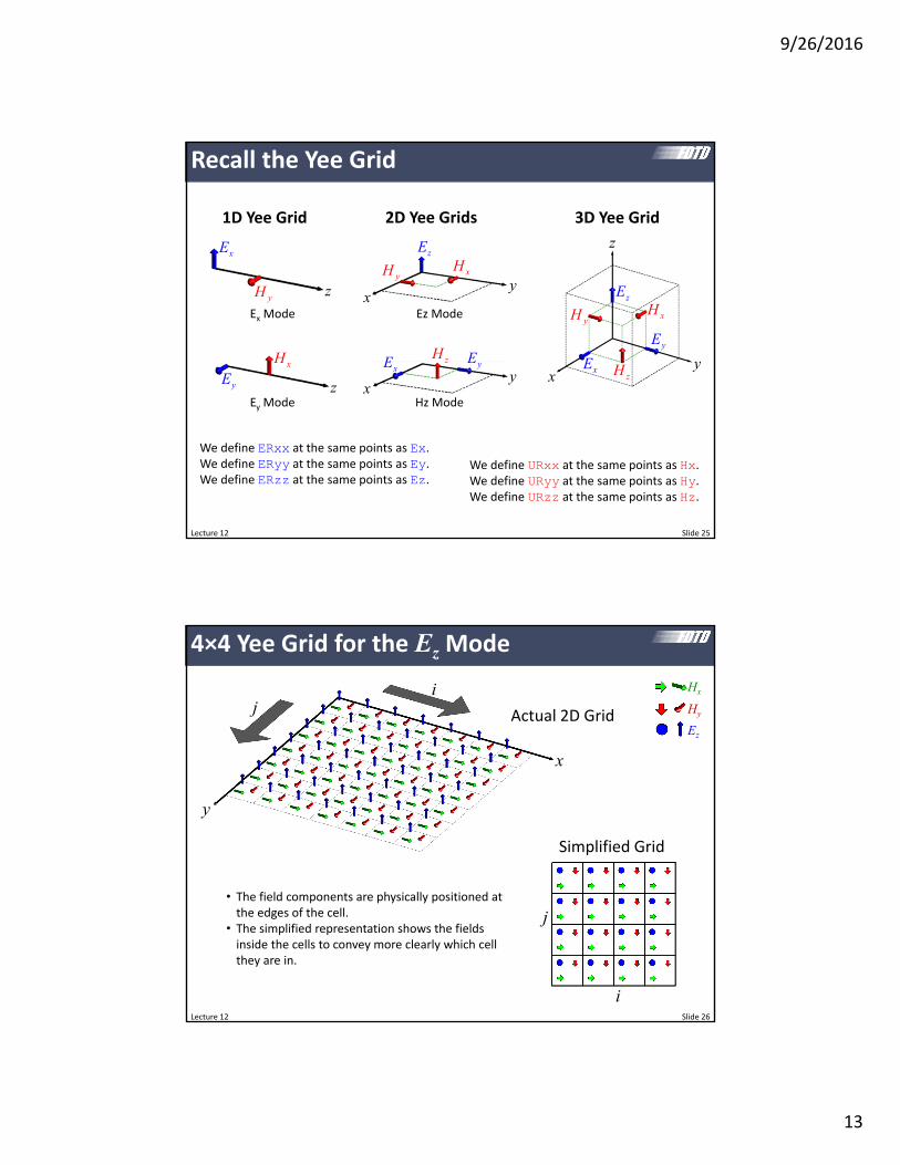
Lecture 12 Slide 25

Recall the Yee Grid

xy

z

xEyE

zE

xHyH

zH

3D Yee Grid2D Yee Grids1D Yee Grid

zE

xHyH

xy

xy

zH yExE

Ez Mode

Hz Mode

z

xE

yH

yExH

Ey Mode

Ex Mode

z

We define ERxx at the same points as Ex.We define ERyy at the same points as Ey.We define ERzz at the same points as Ez.

We define URxx at the same points as Hx.We define URyy at the same points as Hy.We define URzz at the same points as Hz.

Lecture 12 Slide 26

4×4 Yee Grid for the EzMode

Actual 2D Grid

Simplified Grid

• The field components are physically positioned at the edges of the cell.

• The simplified representation shows the fields inside the cells to convey more clearly which cell they are in.

i

j

x

y

Ez

Hy

Hxij

9/26/2016

14

Lecture 12 Slide 27

The 2× Grid

i

j

i

j

The Conventional 1× Grid

y

x

Due to the staggered nature of the Yee grid, 

we are effectively getting twice the 

resolution.

i

j

It now makes sense to talk 

about a grid that is at twice the resolution, the 

“2× grid.”

The 2× grid concept is useful because we can create devices (or PMLs) on the 2× grid without having to think about where the different field components are located.  In a second step, we can easily pull off the values from the 2× grid where they exist for a particular field component.

Ez

Hy

Hx

Lecture 12 Slide 28

2×1× (1 of 4): Define Grids

Suppose we wish to add a circle to our Yee grid.  First, we define the standard 1 grid.

Second, we define a corresponding 2× grid.

Note: the 2× grid represents the same physical space, but with twice the number of points.

9/26/2016

15

Lecture 12 Slide 29

2×1× (2 of 4): Build Device

Third, we construct a cylinder on the 2× grid without having to consider anything about the Yee grid.

Fourth, if desired we could perform dielectric averaging on the 2× grid at this point.

Note: the 2× grid represents the same physical space, but simply with twice the number of points.

Lecture 12 Slide 30

2×1× (3 of 4): Grid Relation

Recall the relation between the 2× and 1× grids as well as the location of the field components.

Ez

Hy

Hx

9/26/2016

16

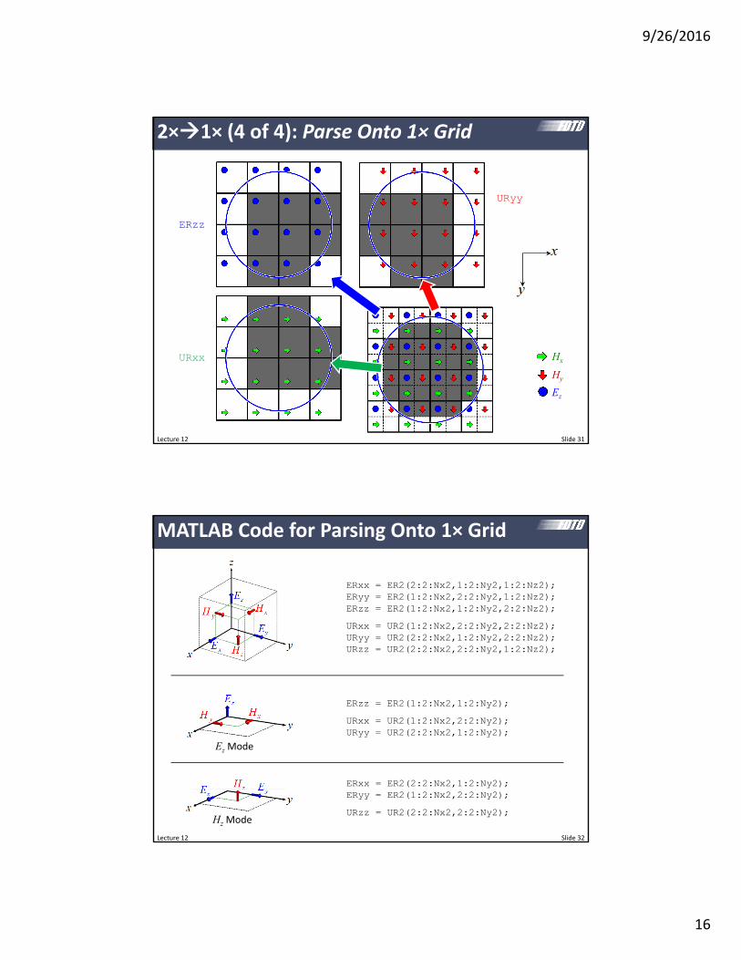
Lecture 12 Slide 31

2×1× (4 of 4): Parse Onto 1× Grid

Ez

Hy

Hx

ERzz

URxx

URyy

Lecture 12 Slide 32

MATLAB Code for Parsing Onto 1× Grid

ERxx = ER2(2:2:Nx2,1:2:Ny2,1:2:Nz2);ERyy = ER2(1:2:Nx2,2:2:Ny2,1:2:Nz2);ERzz = ER2(1:2:Nx2,1:2:Ny2,2:2:Nz2);

URxx = UR2(1:2:Nx2,2:2:Ny2,2:2:Nz2);URyy = UR2(2:2:Nx2,1:2:Ny2,2:2:Nz2);URzz = UR2(2:2:Nx2,2:2:Ny2,1:2:Nz2);

EzMode

ERzz = ER2(1:2:Nx2,1:2:Ny2);

URxx = UR2(1:2:Nx2,2:2:Ny2);URyy = UR2(2:2:Nx2,1:2:Ny2);

HzMode

ERxx = ER2(2:2:Nx2,1:2:Ny2);ERyy = ER2(1:2:Nx2,2:2:Ny2);

URzz = UR2(2:2:Nx2,2:2:Ny2);

9/26/2016

17

Lecture 12 Slide 33

Dielectric Averaging

Lecture 12 Slide 34

What is Dielectric Averaging?

Suppose we have a grid, but the size of the device is not an exact integer number of grid cells.  What can we do?

1 6r 2 1r

Based on the above, we build our device on the grid as follows:

2.5 1 1 1 1 166666666661111

30%

70% ,eff 30% 6.0 70% 1.0 2.5r

r1

= 6

.0

r2 = 1.0

,eff 2.5r

We look at a close‐up of the cell in question and calculate a weighted average.

9/26/2016

18

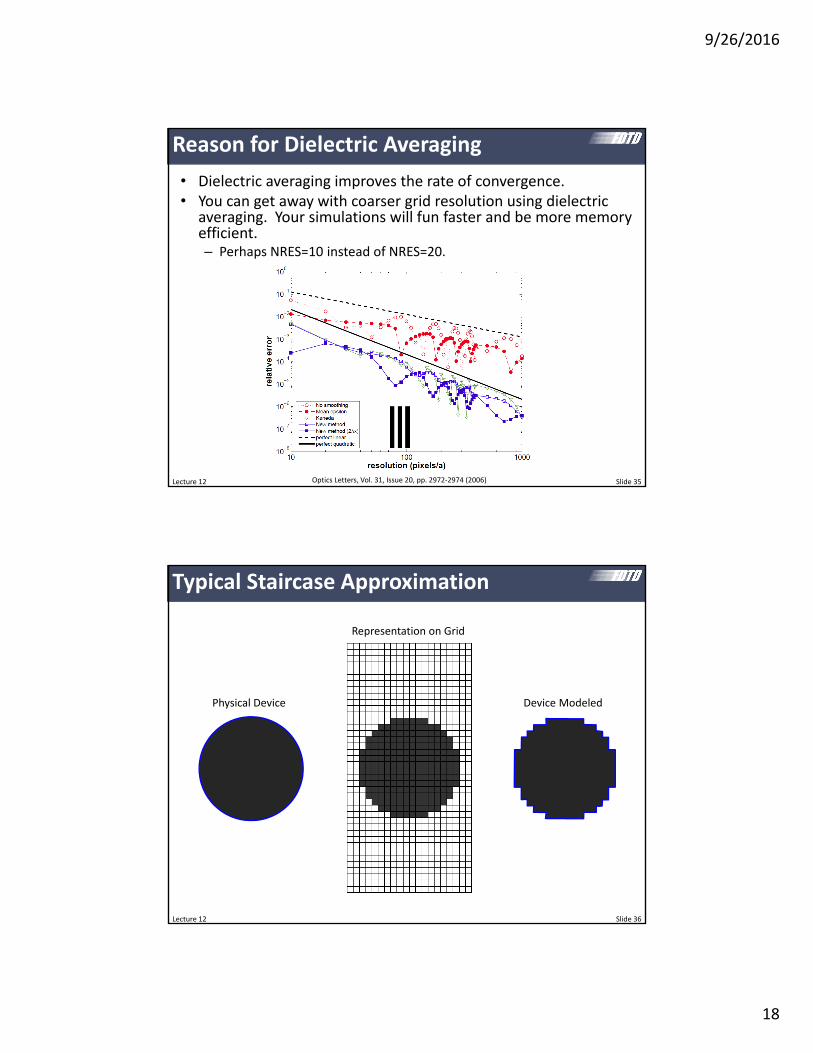
Reason for Dielectric Averaging

• Dielectric averaging improves the rate of convergence.• You can get away with coarser grid resolution using dielectric 

averaging.  Your simulations will fun faster and be more memory efficient.– Perhaps NRES=10 instead of NRES=20.

Lecture 12 Slide 35Optics Letters, Vol. 31, Issue 20, pp. 2972‐2974 (2006)

Lecture 12 Slide 36

Typical Staircase Approximation

Physical Device

Representation on Grid

Device Modeled

9/26/2016

19

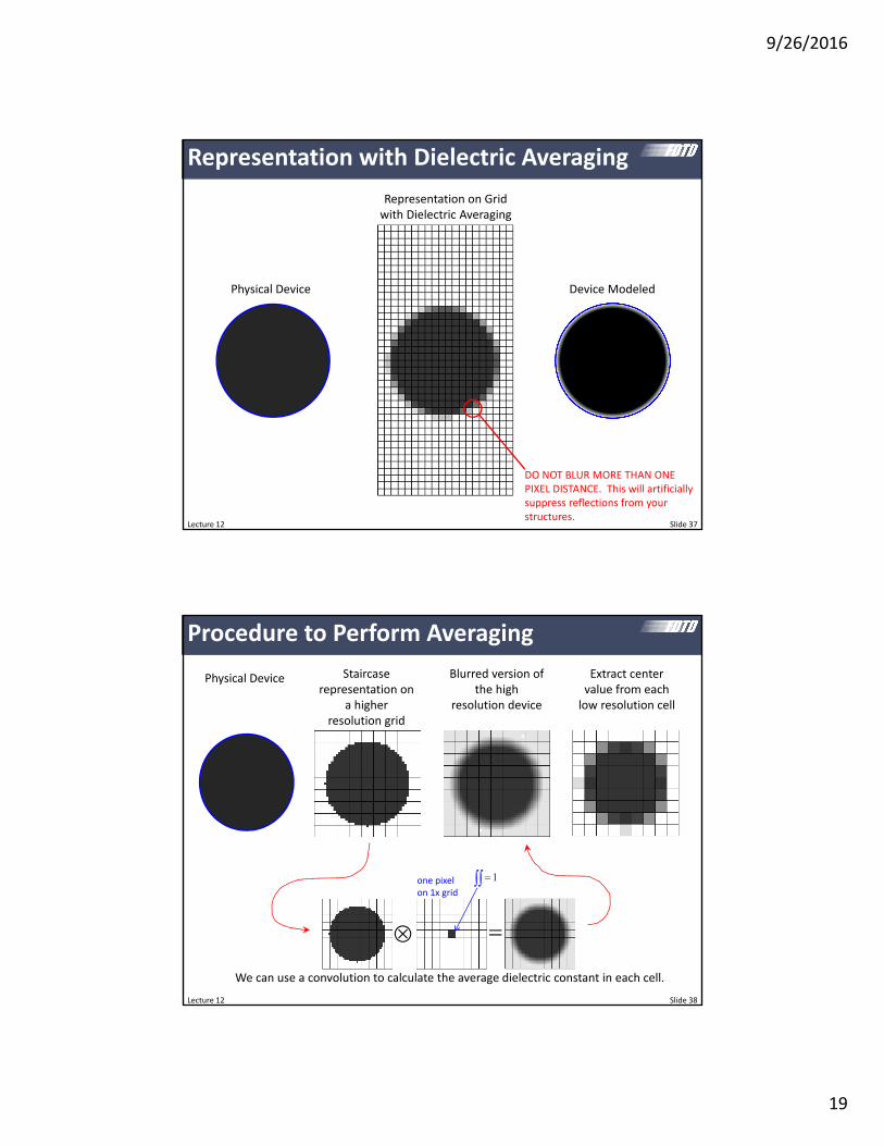
Lecture 12 Slide 37

Representation with Dielectric Averaging

Physical Device

Representation on Gridwith Dielectric Averaging

Device Modeled

DO NOT BLUR MORE THAN ONE PIXEL DISTANCE.  This will artificially suppress reflections from your structures.

Lecture 12 Slide 38

Procedure to Perform Averaging

Physical Device Staircase representation on 

a higher resolution grid

Blurred version of the high 

resolution device

Extract center value from each low resolution cell

1

We can use a convolution to calculate the average dielectric constant in each cell.

one pixel on 1x grid

9/26/2016

20

Lecture 12 Slide 39

Animation of Dielectric Averaging

Lecture 12 Slide 40

Product of Two Functions

Suppose you have the product of two functions that you are approximating numerically.

f z a z b z

Slow convergence is encountered whenever one or both of these functions is discontinuous.

f z a z b z

Suppose a(z) has a discontinuity.  Numerical convergence can be significantly  improved by “smoothing” the discontinuous function at the discontinuity.

9/26/2016

21

Lecture 12 Slide 41

Double Discontinuity (1 of 2)

Suppose both a(z) and b(z) are discontinuous at the same point.  It is very difficult to improve the convergence of this problem.

1f z b z

a z

We can rearrange the equation so that only a single discontinuity exists on each side.

There exists, however, a special case where a(z) and b(z) are discontinuous at the same point, but their product is continuous.  That is, f(z) is continuous.

Lecture 12 Slide 42

Double Discontinuity (2 of 2)

We can now improve convergence by smoothing 1/a(z).

1f z b z

a z

Moving the a(z) term to the right hand side leads to

1

1f z b z

a z

We conclude that in the double discontinuity case where the product is continuous, we smooth the reciprocal of a(z) and then reciprocate the smoothed function.

9/26/2016

22

Lecture 12 Slide 43

Summary of Smoothing

When all functions are continuous, no smoothing is needed.

1

1f z a z b z

f z a z b z

When one of the functions has a step discontinuity, convergence is improved by smoothing that function.

f z a z b z

When both a(z) and b(z) are discontinuous at the same point, but their product is continuous, convergence is improved by smoothing the reciprocal of one of the functions.

Lecture 12 Slide 44

Smoothing and Maxwell’s Equations

In Maxwell’s equations, we have the product of two functions…

rD z z E z

The dielectric function is discontinuous at the interface between two materials.  Boundary conditions require that

1,|| 2,||E E

1 1, 2 2,E E

Tangential component is continuous across the interface

Normal component is discontinuous across the interface, but the product of E is continuous.

We conclude that we must smooth the dielectric function differently for the tangential and normal components.  This implies that the smoothed dielectric function will be anisotropic and described by a tensor.

9/26/2016

23

Lecture 12 Slide 45

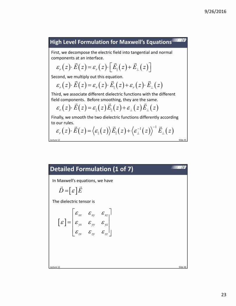
High Level Formulation for Maxwell’s Equations

First, we decompose the electric field into tangential and normal components at an interface.

||r rz E z z E z E z

Second, we multiply out this equation.

||r r rz E z z E z z E z

Third, we associate different dielectric functions with the different field components.  Before smoothing, they are the same.

|| ||r z E z z E z z E z

Finally, we smooth the two dielectric functions differently according to our rules.

11|| ||r z E z z E z z E z

Lecture 12 Slide 46

Detailed Formulation (1 of 7)

In Maxwell’s equations, we have

D E

The dielectric tensor is

xx xy xz

yx yy yz

zx zy zz

9/26/2016

24

Lecture 12 Slide 47

Detailed Formulation (2 of 7)

The electric field can be written as the sum of parallel and perpendicular polarizations.

||E E E

For an arbitrarily shaped device, these components can vary across the grid.  Suppose we could calculate a vector function throughout the grid that is normal to all the interfaces.  This called the “normal vector” field.

ˆ , ,n x y z

P. Gotz, T. Schuster, K. Frenner, S. Rafler, W. Osten, “Normal vector method for the RCWA with automated vector field generation,” Opt. Express 16(22), 17295‐17301 (2008). 

Lecture 12 Slide 48

Detailed Formulation (3 of 7)

The perpendicular component of E can be computed from the normal vector field as follows.

ˆ ˆE n n E

It follows that the parallel component of E is

||

ˆ ˆ

E E E

E n n E

9/26/2016

25

Lecture 12 Slide 49

Detailed Formulation (4 of 7)

In matrix notation, the perpendicular component can be written as

2

2

2

ˆ ˆ

x x x y y z zx

y y x x y y z z

zz x x y y z z

x x y x z x

y x y y z y

z x z y z z

n n E n E n EE

E n n E E n n E n E n E

E n n E n E n E

n n n n n E

n n n n n E

n n n n n E

Lecture 12 Slide 50

Detailed Formulation (5 of 7)

Let

ˆˆ ˆE n n E N E

2

2

2

ˆx x y x z

y x y y z

z x z y z

n n n n n

N n n n n n

n n n n n

The perpendicular and parallel components are then

||ˆ ˆE E N E I N E

9/26/2016

26

Lecture 12 Slide 51

Detailed Formulation (6 of 7)

The constitutive relation can be written in terms of the parallel and perpendicular components of the E field.

||

||

D E E

E E

We smooth the dielectric functions differently according to our rules for optimum convergence.

|| ||

|| ||

D E E

D E E

||

11

Lecture 12 Slide 52

Detailed Formulation (7 of 7)

Putting all of this together leads to

|| ||

||

||

ˆ ˆ

ˆ ˆ

D E E

I N E N E

I N N E

We can derive an effective dielectric tensor from this equation.

smooth ||

|| ||

ˆ ˆ

ˆ

I N N

N

9/26/2016

27

Lecture 12 Slide 53

Summary of Formulation

Given the simulation problem defined by

smooth || || N̂

D E

We can improve the convergence rate by smoothing the dielectric function according to

2

2

2

ˆx x y x z

y x y y z

z x z y z

n n n n n

N n n n n n

n n n n n

||

11

Lecture 12 Slide 54

Dielectric Averaging of a Sphere (1 of 2)

Given a sphere with dielectric constant r=5.0 in air and in a grid with Nx=Ny=Nz=25 cells, the dielectric tensor after averaging is

xy cross section

xz cross section

9/26/2016

28

Lecture 12 Slide 55

Dielectric Averaging of a Sphere (2 of 2)

A 3D visualization is:

xx xy xz

yx yy yz

zx zy zz

Lecture 12 Slide 56

Simulation Example

Recall Exam 1, Problem 1

Response without Smoothing

Response with Smoothing

10 dB improvement

9/26/2016

29

Comments on Dielectric Averaging

• Even if the original dielectric function is isotropic, the averaged dielectric function is anisotropic.

• Anisotropic averaging requires calculating the normal vector field.  This can be difficult, especially for arbitrary structures.

• Convergence still tends to improve even when only isotropic averaging is used.

• The Ezmode does not require anisotropic averaging of the dielectric function.

• The Hzmode does not require anisotropic averaging of the permeability.

Lecture 12 Slide 57

smooth