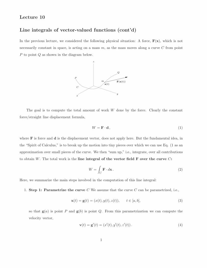
Lecture 10 Line integrals of vector-valued functions (cont…links.uwaterloo.ca/amath231docs/week4.pdf · Line integrals of vector-valued functions (cont’d) ... the “Spirit of

Lecture 10

Line integrals of vector-valued functions (cont’d)

In the previous lecture, we considered the following physical situation: A force, F(x), which is not

necessarily constant in space, is acting on a mass m, as the mass moves along a curve C from point

P to point Q as shown in the diagram below.

C

xy

z

P

Q

F(x(t))x(t)

m

The goal is to compute the total amount of work W done by the force. Clearly the constant

force/straight line displacement formula,

W = F · d , (1)

where F is force and d is the displacement vector, does not apply here. But the fundamental idea, in

the “Spirit of Calculus,” is to break up the motion into tiny pieces over which we can use Eq. (1 as an

approximation over small pieces of the curve. We then “sum up,” i.e., integrate, over all contributions

to obtain W . The total work is the line integral of the vector field F over the curve C:

W =

∫

CF · dx . (2)

Here, we summarize the main steps involved in the computation of this line integral:

1. Step 1: Parametrize the curve C We assume that the curve C can be parametrized, i.e.,

x(t) = g(t) = (x(t), y(t), z(t)), t ∈ [a, b], (3)

so that g(a) is point P and g(b) is point Q. From this parametrization we can compute the

velocity vector,

v(t) = g′(t) = (x′(t), y′(t), z′(t)) . (4)

1

2. Step 2: Compute field vector F(g(t)) over curve C

F(g(t)) = F(x(t), y(t), z(t)) (5)

= (F1(x(t), y(t), z(t), F2(x(t), y(t), z(t), F3(x(t), y(t), z(t))) , t ∈ [a, b] . (6)

3. Step 3: Construct the integrand of∫

C F · dx, i.e., the dot product

F(g(t)) · g′(t) . (7)

4. Step 4: Compute line integral as a definite integral over parameter t

∫

CF · dx =

∫ b

aF(g(t)) · g′(t) dt . (8)

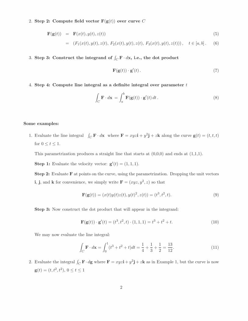
Some examples:

1. Evaluate the line integral∫

C F · dx where F = xyzi + y2j + zk along the curve g(t) = (t, t, t)

for 0 ≤ t ≤ 1.

This parametrization produces a straight line that starts at (0,0,0) and ends at (1,1,1).

Step 1: Evaluate the velocity vector: g′(t) = (1, 1, 1).

Step 2: Evaluate F at points on the curve, using the parametrization. Dropping the unit vectors

i, j, and k for convenience, we simply write F = (xyz, y2, z) so that

F(g(t)) = (x(t)y(t)z(t), y(t)2, z(t)) = (t3, t2, t). (9)

Step 3: Now construct the dot product that will appear in the integrand:

F(g(t)) · g′(t) = (t3, t2, t) · (1, 1, 1) = t3 + t2 + t. (10)

We may now evaluate the line integral:

∫

CF · dx =

∫ 1

0(t3 + t2 + t)dt =

1

4+

1

3+

1

2=

13

12. (11)

2. Evaluate the integral∫

C F · dg where F = xyzi+ y2j+ zk as in Example 1, but the curve is now

g(t) = (t, t2, t2), 0 ≤ t ≤ 1

2

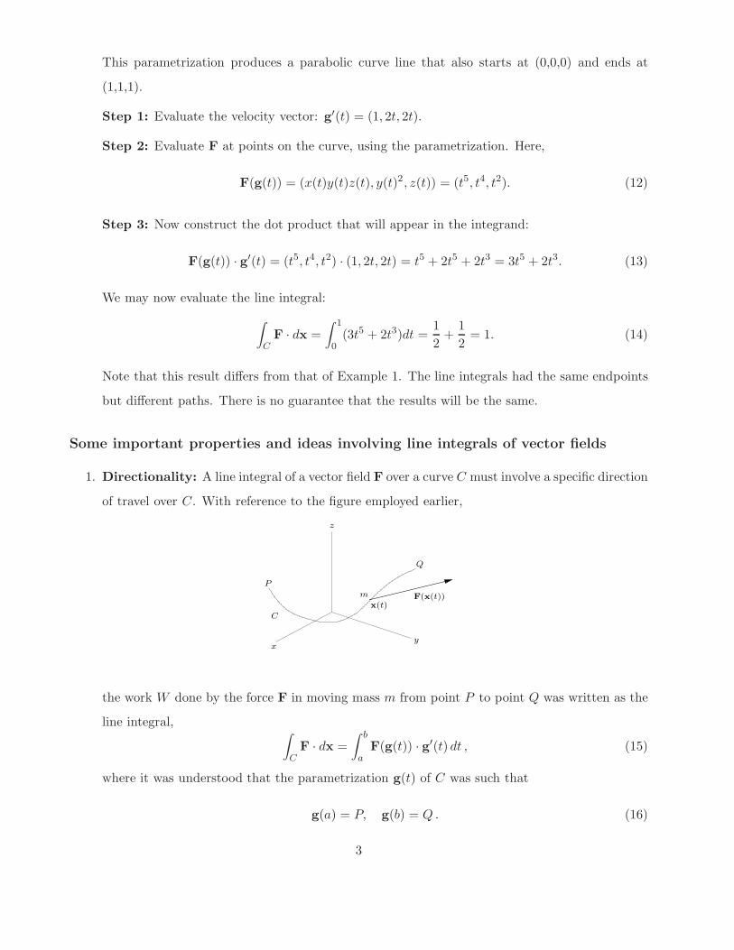
This parametrization produces a parabolic curve line that also starts at (0,0,0) and ends at

(1,1,1).

Step 1: Evaluate the velocity vector: g′(t) = (1, 2t, 2t).

Step 2: Evaluate F at points on the curve, using the parametrization. Here,

F(g(t)) = (x(t)y(t)z(t), y(t)2, z(t)) = (t5, t4, t2). (12)

Step 3: Now construct the dot product that will appear in the integrand:

F(g(t)) · g′(t) = (t5, t4, t2) · (1, 2t, 2t) = t5 + 2t5 + 2t3 = 3t5 + 2t3. (13)

We may now evaluate the line integral:

∫

CF · dx =

∫ 1

0(3t5 + 2t3)dt =

1

2+

1

2= 1. (14)

Note that this result differs from that of Example 1. The line integrals had the same endpoints

but different paths. There is no guarantee that the results will be the same.

Some important properties and ideas involving line integrals of vector fields

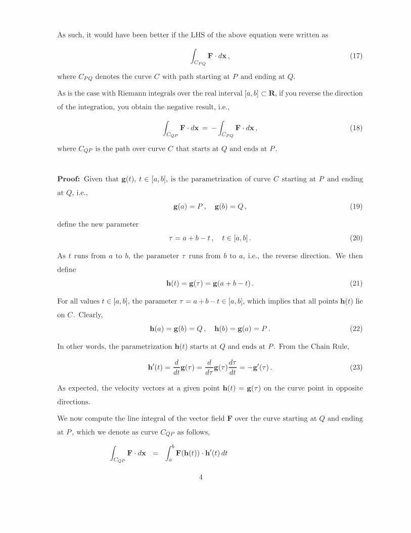
1. Directionality: A line integral of a vector field F over a curve C must involve a specific direction

of travel over C. With reference to the figure employed earlier,

C

xy

z

P

Q

F(x(t))x(t)

m

the work W done by the force F in moving mass m from point P to point Q was written as the

line integral,∫

CF · dx =

∫ b

aF(g(t)) · g′(t) dt , (15)

where it was understood that the parametrization g(t) of C was such that

g(a) = P, g(b) = Q . (16)

3

As such, it would have been better if the LHS of the above equation were written as

∫

CPQ

F · dx , (17)

where CPQ denotes the curve C with path starting at P and ending at Q.

As is the case with Riemann integrals over the real interval [a, b] ⊂ R, if you reverse the direction

of the integration, you obtain the negative result, i.e.,

∫

CQP

F · dx = −

∫

CPQ

F · dx , (18)

where CQP is the path over curve C that starts at Q and ends at P .

Proof: Given that g(t), t ∈ [a, b], is the parametrization of curve C starting at P and ending

at Q, i.e.,

g(a) = P , g(b) = Q , (19)

define the new parameter

τ = a + b − t , t ∈ [a, b] . (20)

As t runs from a to b, the parameter τ runs from b to a, i.e., the reverse direction. We then

define

h(t) = g(τ) = g(a + b − t) . (21)

For all values t ∈ [a, b], the parameter τ = a + b− t ∈ [a, b], which implies that all points h(t) lie

on C. Clearly,

h(a) = g(b) = Q , h(b) = g(a) = P . (22)

In other words, the parametrization h(t) starts at Q and ends at P . From the Chain Rule,

h′(t) =d

dtg(τ) =

d

dτg(τ)

dτ

dt= −g′(τ) . (23)

As expected, the velocity vectors at a given point h(t) = g(τ) on the curve point in opposite

directions.

We now compute the line integral of the vector field F over the curve starting at Q and ending

at P , which we denote as curve CQP as follows,

∫

CQP

F · dx =

∫ b

aF(h(t)) · h′(t) dt

4

=

∫ b

aF(g(a + b − t) · g′(a + b − t) dt

=

∫ a

bF(g(τ) · g′(τ)(−dτ)

(

sincedt

dτ= −1

)

= −

∫ b

aF(g(τ) · g(τ) dτ

= −

∫

CAB

F · dx . (24)

To get from the second-last line to the final line, we note that the parameter τ is being integrated

from a to b. It doesn’t matter what we call the parameter at this point.

Moral of the story: When dealing with the line integral

∫

CF · dx, over a curve C, we must

also specify the orientation of the curve over which the integration is to be performed.

2. Linearity: From the Riemann sum definition of the line integral, it follows that

∫

C(F + G) · dx =

∫

CF · dx +

∫

CG · dx

∫

C(cF) · dx = c

∫

CF · dx , (25)

where c ∈ R is a constant scalar.

3. Additivity over paths: Let C be a C1 curve. (This means that if g(t), t ∈ [a, b], is a

parametrization of C, the tangent vector g′(t) is continuous at all t ∈ [a, b].) Furthermore,

suppose that C may be expressed as a union of two curves C1 and C2 joined end-to-end and

oriented consistently (i.e., orientations of C1 and C2 are compatable), in which case we may

write

C = C1 ∪ C2 . (26)

This is sketched in the figure below. Then

R

C1

C2

C = C1 ∪ C2

P

Q

5

∫

CF · dx =

∫

C1

F · dx +

∫

C2

F · dx . (27)

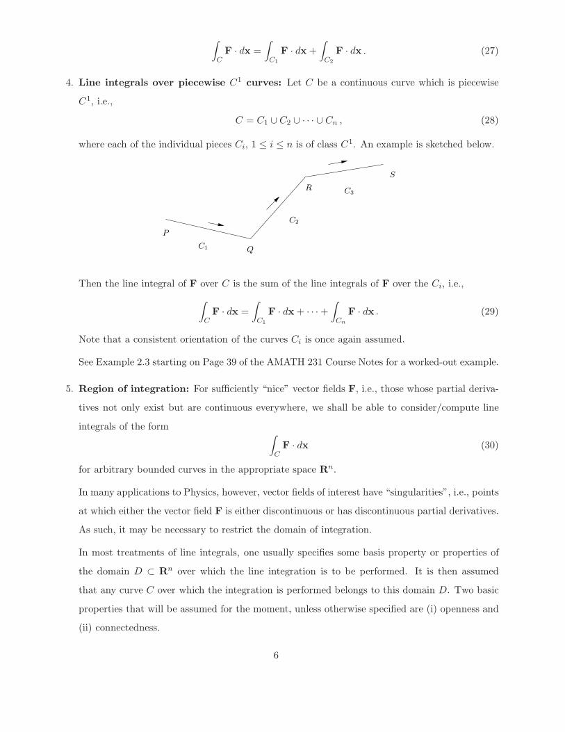
4. Line integrals over piecewise C1 curves: Let C be a continuous curve which is piecewise

C1, i.e.,

C = C1 ∪ C2 ∪ · · · ∪ Cn , (28)

where each of the individual pieces Ci, 1 ≤ i ≤ n is of class C1. An example is sketched below.

C3

P

Q

S

R

C1

C2

Then the line integral of F over C is the sum of the line integrals of F over the Ci, i.e.,

∫

CF · dx =

∫

C1

F · dx + · · · +

∫

Cn

F · dx . (29)

Note that a consistent orientation of the curves Ci is once again assumed.

See Example 2.3 starting on Page 39 of the AMATH 231 Course Notes for a worked-out example.

5. Region of integration: For sufficiently “nice” vector fields F, i.e., those whose partial deriva-

tives not only exist but are continuous everywhere, we shall be able to consider/compute line

integrals of the form∫

CF · dx (30)

for arbitrary bounded curves in the appropriate space Rn.

In many applications to Physics, however, vector fields of interest have “singularities”, i.e., points

at which either the vector field F is either discontinuous or has discontinuous partial derivatives.

As such, it may be necessary to restrict the domain of integration.

In most treatments of line integrals, one usually specifies some basis property or properties of

the domain D ⊂ Rn over which the line integration is to be performed. It is then assumed

that any curve C over which the integration is performed belongs to this domain D. Two basic

properties that will be assumed for the moment, unless otherwise specified are (i) openness and

(ii) connectedness.

6

(a) The set D ⊂ Rn is usually assumed to be an open set in Rn, which may even include the

entire set Rn. When the set D is open, we don’t have to worry about boundaries – given

any point x ∈ D, one can always find an ǫ-neighbourhood of D centered at x for some

ǫ > 0. (Think of the difference between the open interval (a, b) ⊂ R and the closed interval

[a, b] ⊂ R.)

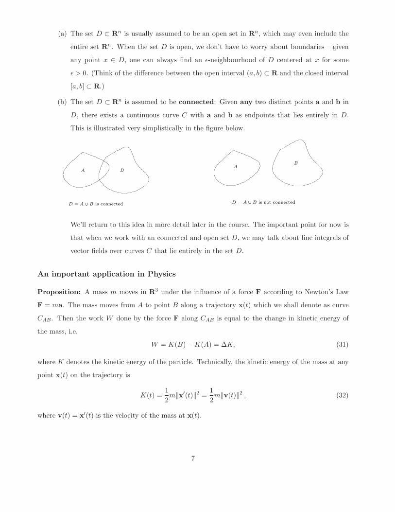
(b) The set D ⊂ Rn is assumed to be connected: Given any two distinct points a and b in

D, there exists a continuous curve C with a and b as endpoints that lies entirely in D.

This is illustrated very simplistically in the figure below.

D = A ∪ B is not connected

A BA

B

D = A ∪ B is connected

We’ll return to this idea in more detail later in the course. The important point for now is

that when we work with an connected and open set D, we may talk about line integrals of

vector fields over curves C that lie entirely in the set D.

An important application in Physics

Proposition: A mass m moves in R3 under the influence of a force F according to Newton’s Law

F = ma. The mass moves from A to point B along a trajectory x(t) which we shall denote as curve

CAB. Then the work W done by the force F along CAB is equal to the change in kinetic energy of

the mass, i.e.

W = K(B) − K(A) = ∆K, (31)

where K denotes the kinetic energy of the particle. Technically, the kinetic energy of the mass at any

point x(t) on the trajectory is

K(t) =1

2m‖x′(t)‖2 =

1

2m‖v(t)‖2 , (32)

where v(t) = x′(t) is the velocity of the mass at x(t).

7

Proof: The total work done by the force is given by the line integral

W =

∫

CAB

F · dx . (33)

Let x(t) = g(t), t ∈ [a, b], denote the parametrization of the trajectory CAB in terms of the time t so

that x(a) = g(a) is point A and x(b) = g(b) is point B. Then

W =

∫

CAB

F · dx (34)

=

∫ b

aF(g(t)) · g′(t) dt,

But g′(t) = v(t) is the velocity of the mass. At all points on the trajectory, Newton’s Law is obeyed,

implying that

F(x(t)) = F(g(t)) = a(t) = mv′(t) . (35)

We substitute this result into the work integral:

W =

∫ b

amv′(t) · v(t) dt. (36)

But recall thatd

dt[v(t) · v(t)] = v′(t) · v(t) + v(t) · v′(t) = 2v′(t) · v(t). (37)

or

v′(t) · v(t) =1

2

d

dt[v(t) · v(t)] =

1

2

d

dt‖ v(t) ‖2 . (38)

Therefore

W =1

2m

∫ b

a

d

dt‖ v(t) ‖2 dt (39)

=1

2m ‖ v(b) ‖2 −

1

2m ‖ v(a) ‖2

= K(B) − K(A)

= ∆K.

You probably saw this result for one-dimensional motion in your first-year Physics course. Note,

however, that we have not made any assumptions on F – it does not have to be conservative. For

example, it also holds for frictional forces, which are nonconservative. The proof of this result for

conservative forces is much simpler, since we can use the fact that total mechanical energy is conserved.

But we must make use of the Fundamental Theorems for Line Integrals, the next topic.

8

Path-independence and the Fundamental Theorems of Calculus for

Line Integrals

(Relevant section from AMATH 231 Course Notes: 2.3)

We begin with some additional examples of line integrals of vector-valued functions, which will moti-

vate the discussion.

Examples:

1. Evaluate the line integral∫

C F·dx where F = 2xi+4yj+zk along the curve g(t) = (cos t, sin t, t),

with 0 ≤ t ≤ 2π.

This parametrization produces a helical curve that starts at (1, 0, 0) and ends at (1, 0, 2π).

Step 1: Evaluate the velocity vector: g′(t) = (− sin t, cos t, 1).

Step 2: Evaluate F at points on the curve:

F(g(t)) = (2x(t), 4y(t), z(t)) = (2 cos t, 4 sin t, t) (40)

Step 3: Now construct the dot product that will appear in the integrand:

F(g(t)) · g′(t) = (2 cos t, 4 sin t, t) · (− sin t, cos t, 1) = 2 cos t sin t + t (41)

Now evaluate the line integral:

∫

CF · dx =

∫ 2π

0(2 cos t sin t + t) dt (42)

=

[

sin2 t +1

2t2

]2π

0

= 2π2.

2. Now evaluate the line integral∫

C F · dx, where F is the vector field used in Example 1, but

the curve is now the straight line from (1, 0, 0) to (1, 0, 2π). Since the value of the line integral

is independent of the parametrization used, we’ll use the simplest one, g(t) = (1, 0, t), with

0 ≤ t ≤ 2π.

Step 1: Evaluate the velocity vector: g′(t) = (0, 0, 1).

9

Step 2: Evaluate F at points on the curve, using the parametrization. Here,

F(g(t)) = (2x(t), 4y(t), z(t)) = (2, 0, t). (43)

Step 3: Now construct the dot product that will appear in the integrand:

F(g(t)) · g′(t) = (2, 0, t) · (0, 0, 1) = t (44)

Now evaluate the line integral:

∫

CF · dx =

∫ 2π

0t dt = 2π2. (45)

Note that the results of Examples 1 and 2 are identical. This could be a coincidence but if you

tried other paths with the same endpoints, you would obtain 2π2. We’ll show very shortly that for

vector field F = (x, 2y, 4z), the line integral

∫

CF · dx = 2π2 (46)

for any (piecewise C1) path that starts at (1, 0, 0) and ends at (1, 0, 2π). In other words, the line

integral is independent of path or simply path-independent.

The reason for this path-independence is the fact that the vector field F examined above is a

gradient field, i.e., there exists a scalar function f(x, y, z) such that F = ~∇f . (Recall that physicists

prefer to think of a conservative field, i.e., a vector field F = −~∇V for some scalar function

V (x, y, z).) In this case,

F = 2xi + 4yj + zk = ~∇f, (47)

where

f(x, y, z) = x2 + 2y2 +1

2z2 + C, (48)

for any constant C ∈ R.

Here is our claim, which is Theorem 2.2 in the AMATH 231 Course Notes, p. 45, the so-called Second

Fundamental Theorem for Line Integrals:

Theorem: Let F : D → Rn be a continuous vector field on a connected and open set D ⊂ Rn, and

let x1 and x2 be any two points in D. Furthermore, assume that F is a gradient field, i.e., F = ~∇f ,

where f : D → R is a C1 scalar field. Now let C be any curve in D which joins x1 and x2 (in other

10

words, the endpoints of C are x1 and x2) and let the orientation of the integration over C be from x1

(start) to x2 (finish). Then

∫

CF · dx =

∫

C

~∇f · dx = f(x2) − f(x1) (f(finish) − f(start)) . (49)

Note that the line integral depends only on the endpoints x1 and x2 and not on the

path C taken.

We’ll often state this result as follows:

∫

CAB

F · dx =

∫

CAB

~∇f · dx = “f(B) − f(A)′′, (50)

where CAB denotes a curve that starts at A and ends at B, and f(A) and f(B) denote the values of

f at these respective endpoints.

Here, we can also comment that the above Theorem also implies the following relationship,

∫

CBA

~∇f · dx = f(A) − f(B) = − [f(B) − f(A)] = −

∫

CAB

~∇f · dx , (51)

where CBA is any curve that starts at B and ends at A.

Note: In these lecture notes, we shall often refer to the Second Fundamental Theorem

for Line Integrals in abbreviated form as “FTLI 2”.

Why “Second Fundamental Theorem for Line Integrals”? Let’s go back to the Second Fundamental

Theorem of Calculus (FTC II) for functions of a single variable, which implies that

∫ b

af ′(x) dx = f(b) − f(a), (52)

since f(x) is an antiderivative of f ′(x). Comparing (52) and (49) it appears that the gradient of f ,

~∇f , is the “natural derivative” of a function f of several variables. (Of course, for the single variable

case, it is the derivative of f : ~∇f = f ′(x)i.)

Proof of the above Theorem: Let C be given by the parametrization

x(t) = g(t), t1 ≤ t ≤ t2 , (53)

11

so that

x1 = g(t1), x2 = g(t2) . (54)

(Note: We do not have to come up with a particular parametrization. The knowledge that such a

parametrization exists is sufficient for the proof.)

Then

∫

C

~∇f · dx =

∫ t2

t1

~∇f(g(t)) · g′(t) dt

=

∫ t2

t1

d

dt[f(g(t))] dt (Chain Rule)

= f(g(t2)) − f(g(t1)) (FTC II for integrals over R)

= f(x2) − f(x1) (55)

and the theorem is proved.

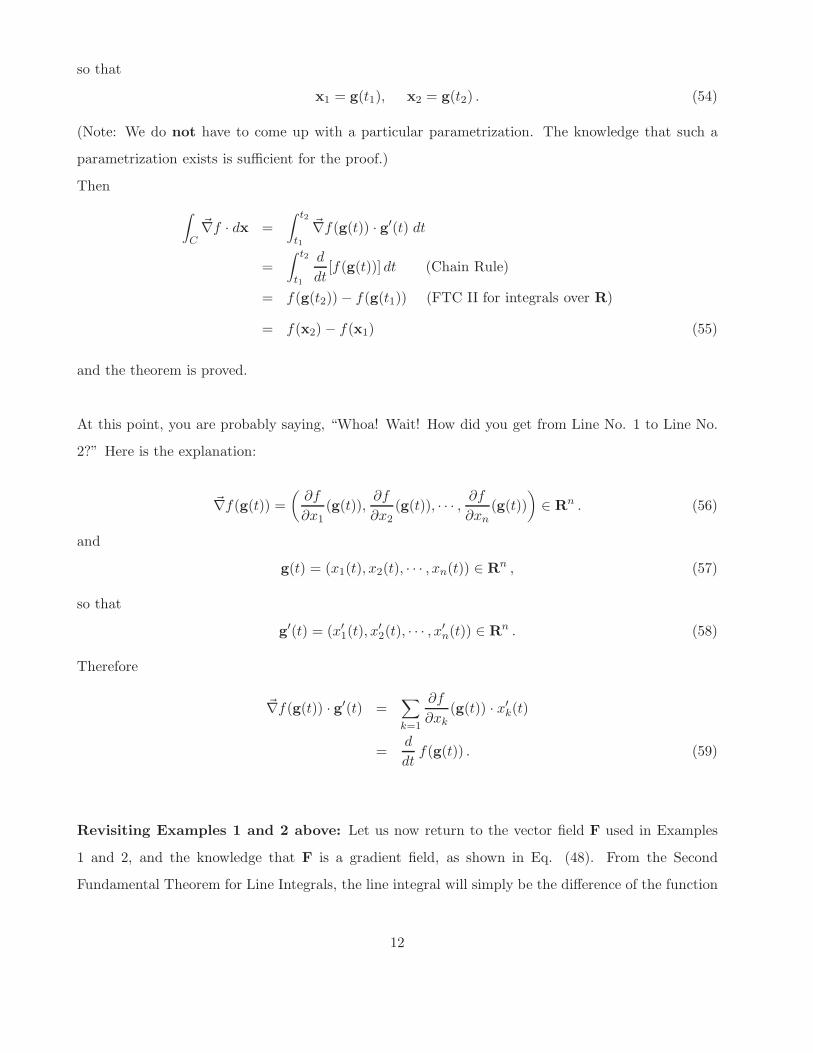
At this point, you are probably saying, “Whoa! Wait! How did you get from Line No. 1 to Line No.

2?” Here is the explanation:

~∇f(g(t)) =

(

∂f

∂x1(g(t)),

∂f

∂x2(g(t)), · · · ,

∂f

∂xn

(g(t))

)

∈ Rn . (56)

and

g(t) = (x1(t), x2(t), · · · , xn(t)) ∈ Rn , (57)

so that

g′(t) = (x′

1(t), x′

2(t), · · · , x′

n(t)) ∈ Rn . (58)

Therefore

~∇f(g(t)) · g′(t) =∑

k=1

∂f

∂xk

(g(t)) · x′

k(t)

=d

dtf(g(t)) . (59)

Revisiting Examples 1 and 2 above: Let us now return to the vector field F used in Examples

1 and 2, and the knowledge that F is a gradient field, as shown in Eq. (48). From the Second

Fundamental Theorem for Line Integrals, the line integral will simply be the difference of the function

12

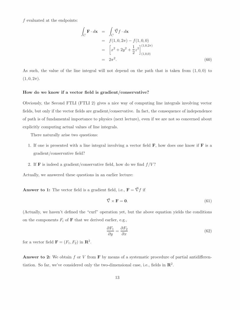
f evaluated at the endpoints:

∫

CF · dx =

∫

C

~∇f · dx

= f(1, 0, 2π) − f(1, 0, 0)

=

[

x2 + 2y2 +1

2z2

](1,0,2π)

(1,0,0)

= 2π2. (60)

As such, the value of the line integral will not depend on the path that is taken from (1, 0, 0) to

(1, 0, 2π).

How do we know if a vector field is gradient/conservative?

Obviously, the Second FTLI (FTLI 2) gives a nice way of computing line integrals involving vector

fields, but only if the vector fields are gradient/conservative. In fact, the consequence of independence

of path is of fundamental importance to physics (next lecture), even if we are not so concerned about

explicitly computing actual values of line integrals.

There naturally arise two questions:

1. If one is presented with a line integral involving a vector field F, how does one know if F is a

gradient/conservative field?

2. If F is indeed a gradient/conservative field, how do we find f/V ?

Actually, we answered these questions in an earlier lecture:

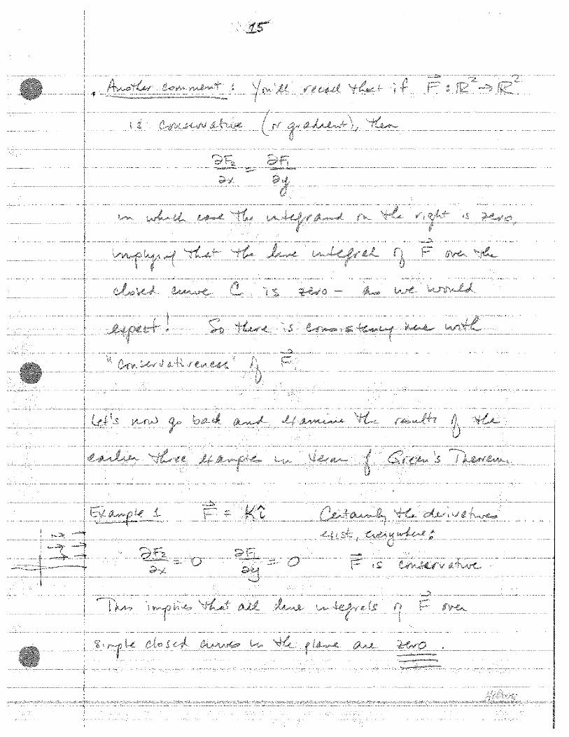
Answer to 1: The vector field is a gradient field, i.e., F = ~∇f if

~∇× F = 0. (61)

(Actually, we haven’t defined the “curl” operation yet, but the above equation yields the conditions

on the components Fi of F that we derived earlier, e.g.,

∂F1

∂y=

∂F2

∂x(62)

for a vector field F = (F1, F2) in R2.

Answer to 2: We obtain f or V from F by means of a systematic procedure of partial antidifferen-

tiation. So far, we’ve considered only the two-dimensional case, i.e., fields in R2.

13

Lecture 11

Line integrals of vector-valued functions (cont’d)

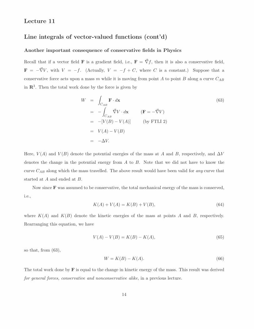
Another important consequence of conservative fields in Physics

Recall that if a vector field F is a gradient field, i.e., F = ~∇f , then it is also a conservative field,

F = −~∇V , with V = −f . (Actually, V = −f + C, where C is a constant.) Suppose that a

conservative force acts upon a mass m while it is moving from point A to point B along a curve CAB

in R3. Then the total work done by the force is given by

W =

∫

CAB

F · dx (63)

= −

∫

CAB

~∇V · dx (F = −~∇V )

= −[V (B) − V (A)] (by FTLI 2)

= V (A) − V (B)

= −∆V.

Here, V (A) and V (B) denote the potential energies of the mass at A and B, respectively, and ∆V

denotes the change in the potential energy from A to B. Note that we did not have to know the

curve CAB along which the mass travelled. The above result would have been valid for any curve that

started at A and ended at B.

Now since F was assumed to be conservative, the total mechanical energy of the mass is conserved,

i.e.,

K(A) + V (A) = K(B) + V (B), (64)

where K(A) and K(B) denote the kinetic energies of the mass at points A and B, respectively.

Rearranging this equation, we have

V (A) − V (B) = K(B) − K(A), (65)

so that, from (63),

W = K(B) − K(A). (66)

The total work done by F is equal to the change in kinetic energy of the mass. This result was derived

for general forces, conservative and nonconservative alike, in a previous lecture.

14

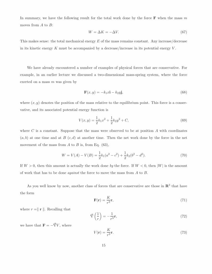
In summary, we have the following result for the total work done by the force F when the mass m

moves from A to B:

W = ∆K = −∆V. (67)

This makes sense: the total mechanical energy E of the mass remains constant. Any increase/decrease

in its kinetic energy K must be accompanied by a decrease/increase in its potential energy V .

We have already encountered a number of examples of physical forces that are conservative. For

example, in an earlier lecture we discussed a two-dimensional mass-spring system, where the force

exerted on a mass m was given by

F(x, y) = −k1xi − k2yj, (68)

where (x, y) denotes the position of the mass relative to the equilibrium point. This force is a conser-

vative, and its associated potential energy function is

V (x, y) =1

2k1x

2 +1

2k2y

2 + C, (69)

where C is a constant. Suppose that the mass were observed to be at position A with coordinates

(a, b) at one time and at B (c, d) at another time. Then the net work done by the force in the net

movement of the mass from A to B is, from Eq. (63),

W = V (A) − V (B) =1

2k1(a

2 − c2) +1

2k2(b

2 − d2). (70)

If W > 0, then this amount is actually the work done by the force. If W < 0, then |W | is the amount

of work that has to be done against the force to move the mass from A to B.

As you well know by now, another class of forces that are conservative are those in R3 that have

the form

F(r) =K

r3r, (71)

where r =‖ r ‖. Recalling that

~∇

(

1

r

)

= −1

r3r, (72)

we have that F = −~∇V , where

V (r) =K

r3r. (73)

15

1. F(r) =Qq

4πǫ0r3r, the electrostatic force on a charge q at r due to a charge Q at the origin 0.

Here, K =Qq

4πǫ0so that the potential energy function is V (r) =

Qq

4πǫ0r.

2. F(r) = −GMm

r3r, the gravitational force on a mass m at r due to a mass M at the origin 0.

Here, K = −GMm so that the potential energy function is V (r) = −GMm

r.

It’s worth pointing out that earlier in this course, we “discovered” that these forces were conser-

vative from the gradient relation in (72). We were spared the work of trying to find the potential

functions associated with these forces, i.e., by first checking if the forces were conservative (using the

curl test) and then integrating backwards to find the potential functions.

Here’s an application that you’ve no doubt seen in first-year Physics: Suppose that a satellite

moves from point A in space to point B along a curve CAB under the influence of the earth’s gravity.

What is the work done by gravity?

We assume (and correctly so, as we’ll prove later) that we can treat the earth as a point mass M

that defines the origin O of our fixed coordinate system. Using the results from a couple of paragraphs

above, the answer is simply

W = V (A) − V (B) = −GMm

rA

+GMm

rB

= GMm

[

−1

rA

+1

rB

]

, (74)

where rA = |OA| and rB = |OB| are the radial distances between the earth (origin O) and the satellite

at points A and B.

Some notes:

1. If rA = rB , then W = 0.

2. If rA > rB (i.e., the satellite has moved inward), then W > 0. The work done by gravity is

positive (decrease in potential energy).

3. If rA < rB (i.e., the satellite has moved outward), then W < 0. The work done by gravity is

negative (increase in potential energy).

It is certainly possible that all of these situations can be encountered during a single orbit of the

satellite around the earth. For example,

16

1. If the orbit is perfectly circular, then rA = rB = r, a constant, during the entire orbit, which

means that no work is ever done.

2. If the orbit is elliptical, then pick two points on the orbit such that rA > rB . In travelling from

A to B, work has been done by gravity (decrease in potential energy). In returning to A from B,

an equal amount of work has been done against gravity (implying an equal increase in potential

energy). The motion along an elliptical orbit involves a constant interchange between potential

and kinetic energy.

17

First Fundamental Theorem for Line Integrals (FTLI 1)

Recall the First Fundamental Theorem of Calculus (or FTC I): If a function f is continuous on [a,b],

then the function g defined on [a, b] as follows,

g(x) =

∫ x

af(t) dt, a ≤ x ≤ b , (75)

is an antiderivative of f , i.e.

g′(x) = f(x) . (76)

In particular, g is the unique antiderivative of f for which

g(a) = 0 . (77)

As in the case of FLTI 2, there is a corresponding First Fundamental Theorem for Line Integrals,

or “FTLI 1”. The natural question is: What is the line integral analogue of Eq. (75) in which

f : R → R is replaced by a vector field F : Rn → Rn and the points a and x in R are replaced by

suitable points in Rn?

The answer is that the line integral

∫

CF · dx must be path-independent. In this case, we define a

scalar field f : Rn → R as follows,

f(x) =

∫

x

x0

F · dy , (78)

where y is a dummy integration variable in Rn. Note that we do not have to specify a curve C over

which the above integration is performed since the line integral is assumed to be independent of the

path from x0 to x. In this case, subject to some additional assumptions,

~∇f = F . (79)

In other words, F is a gradient field and f is viewed as a kind of antiderivative of F.

Let us now state and prove the FTLI 1, which is Theorem 2.1 in the AMATH Course Notes, p. 43.

Theorem Let F : D → Rn be a continuous vector field on a connected and open subset D ⊂ Rn.

Furthermore assume that all line integrals over F are path dependent in D. Now define the scalar-

valued function f : D → Rn as follows,

f(x) =

∫

x

x0

F · dy , (80)

18

for all x ∈ D, where x0 is a specified point in D. Then

~∇f(x) = F(x) for all x ∈ D . (81)

Note: In these notes, we use f to denote the scalar field. In the AM231 Course Notes, φ is used to

denote the scalar field.

Proof: (We follow the proof presented in the AMATH Course Notes quite closely.) We consider the

case R2 for simplicity. An extension of the proof to the general case Rn is possible, using the same

basic ideas.

We must prove that for f defined in (80), Eq. (81) holds componentwise, i.e.,

∂f

∂x= F1 ,

∂f

∂y= F2 , (82)

where F1 and F2 are the components of F, i.e., F = (F1, F2).

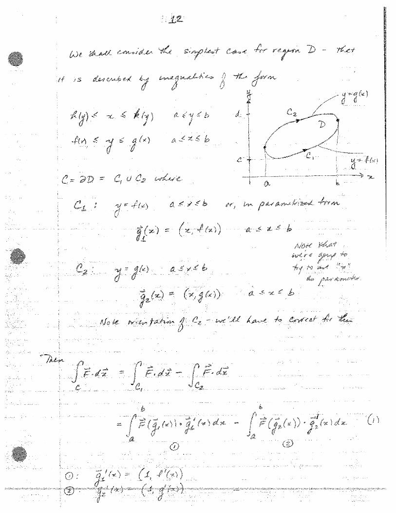
Since line integrals over F in D are assumed to be path-independent, we may employ a special

curve C that runs from x0 = (x0, y0) to x = (x, y), both in D. The curve C = C1 ∪ C2, composed of

two segments, is shown in the figure below.

(x0, y)

C1

C2

x

y

(x, y)

(x0, y0)

The following simple parametrizations for the segments comprising C will be employed:

x(t) = g1(t) = (x0, t), y0 ≤ t ≤ y , Curve C1 ,

x(t) = g1(t) = (t, y), x0 ≤ t ≤ x , Curve C2 . (83)

From the additivity property of the line integral,

f(x, y) =

∫

CF · dy

19

=

∫

C1

F · dy +

∫

C2

F · dy

=

∫ (x0,y)

(x0,y0)F · dy +

∫ (x,y)

(x0,y)F · dy

= LI1 + LI2 . (84)

From the definition of the line integral, the component line integrals LI1 and LI2 over C1 and C2,

respectively, may be written as follows,

LI1 =

∫ y

y0

F(g1(t)) · g′

1(t) dt (85)

and

LI2 =

∫ x

x0

F(g2(t)) · g′

2(t) dt (86)

We now compute the integrands in each component line integral, first computing the velocity vectors

associated with each parametrization,

g′

1(t) = (0, 1), g′

2(t) = (1, 0) . (87)

(These results should be clear from the figure above.) The integrand in LI1 then becomes

(F1(x(t), y(t)), F2(x(t), y(t)) · (0, 1) = F2(x(t), y(t)) = F2(x0, t) , (88)

and the integrand in LI2 becomes

(F1(x(t), y(t)), F2(x(t), y(t))) · (1, 0) = F1(x(t), y(t)) = F1(t, y) . (89)

Substitution into (85) and (86) yields

LI1 =

∫ y

y0

F2(x0, t) dt , LI2 =

∫ x

x0

F1(t, y) dt . (90)

From Eq. (84), we have

f(x, y) =

∫ y

y0

F2(x0, t) dt +

∫ x

x0

F1(t, y) dt . (91)

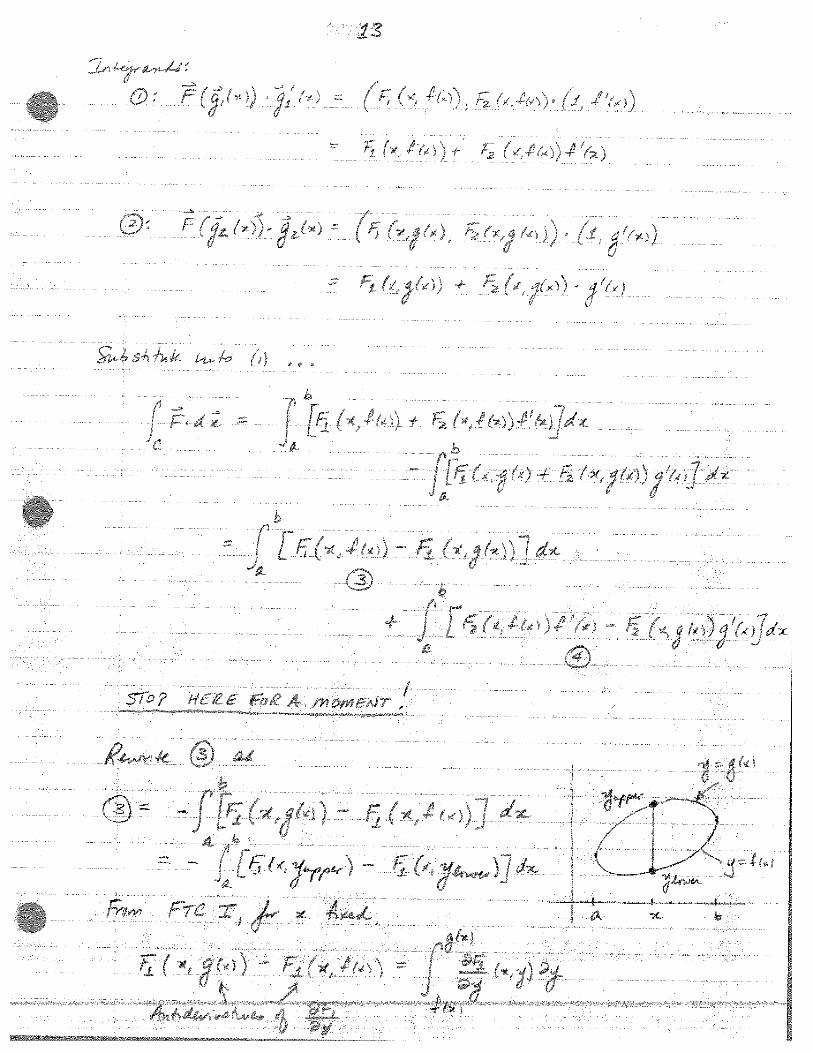
Note that the first definite integral in Eq. (91) is independent of x. We take the partial derivatives of

both sides with respect to x, treating, of course, y as a constant, to obtain

∂f

∂x=

∂

∂x

[∫ y

y0

F2(x0, t) dt

]

+∂

∂x

[∫ x

x0

F1(t, y) dt

]

. (92)

The first term on the RHS is zero. The second term may be evaluated by means of the first Funda-

mental Theorem of Calculus for Riemann integrals to yield the result,

∂f

∂x= F1(x, y) . (93)

20

We have accomplished one-half of our goal in Eq. (82).

Unfortunately, if we try to compute the other partial derivative from (91),

∂f

∂y= F2(x0, y) +

∫ x

x0

∂F1

∂y(t, y) dt , (94)

we can go no further, i.e., we cannot show that the RHS is equal to F2(x, y). In fact, it is not even

guaranteed that the integral in this equation exists. The only assumption on the vector field F is that

it is continuous. As such, there is no guarantee that the integrand∂F1

∂yis a continuous function, or

that it even exists!

Fortunately, the other relation in Eq. (82) may be derived if we employ a different integration

path – the one sketched in the figure below.

x

y

(x, y)

(x0, y0)

C1

C2

(x, y0)

By means of a procedure quite analogous to the one used above, we arrive at the desired result, namely,

∂f

∂y= F2(x, y) , (95)

and the proof is complete.

A note regarding Eqs. (94) and (95) in the above proof

If we make the additional assumption that the vector field F in the above Theorem has continuous

partial derivatives, then the integral in Eq. (94) exists. From Eqs. (94) and (95), it then follows that

F2(x, y) = F2(x0, y) +

∫ x

x0

∂F1

∂y(t, y) dt , (96)

which may seem to be a rather strange result.

Note that the first term on the RHS of Eq. (96) is independent of x. Now take the partial

derivatives of both sides of this equation with respect to x to obtain

∂F2

∂x(x, y) = 0 +

∂

∂x

[∫ x

x0

∂F1

∂y(t, y) dt

]

=∂F1

∂y(x, y) . (97)

21

Recall that we derived this condition – assuming that the partial derivatives are continuous functions

- for the vector field F to be a gradient field, i.e., that F = ~∇f for a scalar field f .

Unfortunately, we could not use this result in the proof, since no assumption was made on the

existence of partial derivatives of the Fi.

Application of FTLI 1 to Physics

Recall that in Physics, it is more convenient to consider a vector field F : Rn → Rn, often a force

field, as a conservative field instead of a gradient field. Let us recall that a C1 vector field F is

conservative if the partial derivatives of its components satisfy a set of relations. For example, in R2,

where F = (F1, F2), these relations are∂F1

∂y=

∂F2

∂x. (98)

In this case, there exists a scalar field V : Rn → R, commonly known as the potential associated

with F, such that

F = −~∇V (= ~∇f) . (99)

(Once again, we simply replace f of the previous section with −V .)

We have already discussed the consequences of the Second Fundamental Theorem for Line Integrals

for conservative forces in a previous section. Here, we examine the implications of FTLI 1. If F is

conservative, then we may define the associated potential function V (x) as follows,

f(x) = −V (x) =

∫

x

x0

F · dy , (100)

where x0 is a suitable reference point. This then leads to

V (x0) = −

∫

x

x0

F · dy . (101)

Once again, the value of the potential function V at x may be interpreted as the work done against

the force F in moving a mass from the reference point x0 to point x. No curve C need be

specified in the above line integral because the line integral is path-independent. Note also that

V (x0) = 0 . (102)

From Eq. (101) and the FTLI 1, it follows that

~∇V = −F , (103)

22

from which Eq. (99) follows.

Eq. (101) is the n-dimensional extension of the one-dimensional result that we discussed in

an earlier lecture: If a force F = f(x)i is acting on a mass that can move only in one dimension

(represented by the x-axis), then the potential energy associated with this force is

V (x) = −

∫ x

af(s) ds , (104)

where a is a suitable reference point. Furthermore, from the First Fundamental Theorem of Calculus

for Riemann integrals,

V ′(x) = −f(x) =⇒ f(x) = −V ′(x) . (105)

23

Line integrals of vector fields over closed curves

Let us recall the Second Fundamental Theorem for Line Integrals, proven in a previous section:

Theorem: Let F : D → Rn be a continuous vector field on a connected and open set D ⊂ Rn, and

let a and b be any two points in D. Furthermore, assume that F is a gradient field, i.e., F = ~∇f ,

where f : D → R is a C1 scalar field. Now let C be any curve in D which joins a and b (in other

words, the endpoints of C are a and b) and let the orientation of the integration over C be from a

(start) to b (finish). Then

∫

CF · dx =

∫

C

~∇f · dx = f(b) − f(a) (f(finish) − f(start)) . (106)

As mentioned in the previous section, the line integral depends only on the endpoints a and b

and not on the path C taken.

We now ask the question, what happens if we start from a, go away for a while (e.g., sixth floor

of MC, Student Life Centre, etc.) and then return to a. This, of course, implies that b = a and the

above result becomes∫

CF · dx =

∫

C

~∇f · dx = f(a) − f(a) = 0 . (107)

This will be the case if the conditions of the theorem are satisfied, i.e., the vector field F is continuous

and a gradient field over the region that you have travelled.

If F is a conservative force, e.g., gravity, in which case f = −V , where V is the potential energy

function, then the above leads to the important conclusion that no net work was done, either by

the force or against the force.

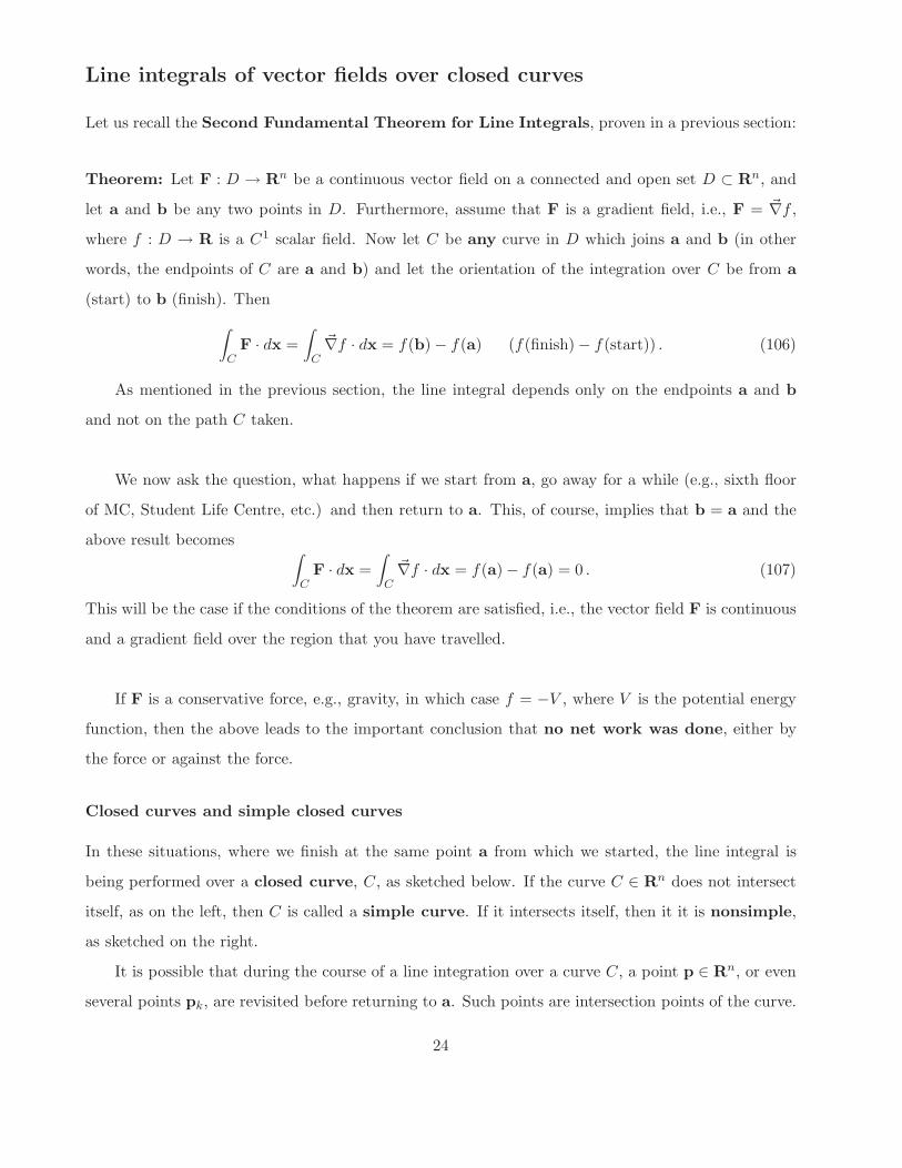
Closed curves and simple closed curves

In these situations, where we finish at the same point a from which we started, the line integral is

being performed over a closed curve, C, as sketched below. If the curve C ∈ Rn does not intersect

itself, as on the left, then C is called a simple curve. If it intersects itself, then it it is nonsimple,

as sketched on the right.

It is possible that during the course of a line integration over a curve C, a point p ∈ Rn, or even

several points pk, are revisited before returning to a. Such points are intersection points of the curve.

24

.

.

.a

p

a

C

C

Left: Simple closed curve. Right: Nonsimple closed curve.

For much of this course, however, we shall be concerned mostly with line integrals of vector fields over

simple closed curves (in Rn).

The usual notation for a line integral over a simple closed curve C is

∮

CF · dx . (108)

(That being said, this notation is not employed in the AMATH 231 Course Notes, but it will be

employed in these lecture notes.)

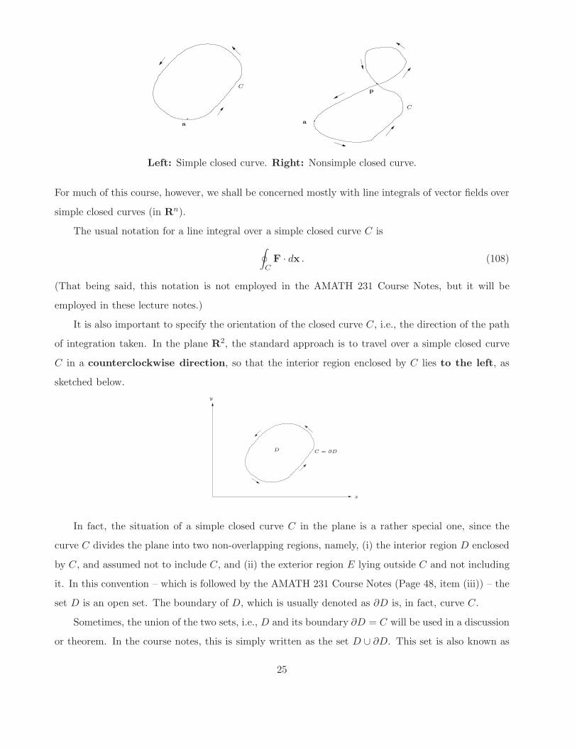
It is also important to specify the orientation of the closed curve C, i.e., the direction of the path

of integration taken. In the plane R2, the standard approach is to travel over a simple closed curve

C in a counterclockwise direction, so that the interior region enclosed by C lies to the left, as

sketched below.

y

D

x

C = ∂D

In fact, the situation of a simple closed curve C in the plane is a rather special one, since the

curve C divides the plane into two non-overlapping regions, namely, (i) the interior region D enclosed

by C, and assumed not to include C, and (ii) the exterior region E lying outside C and not including

it. In this convention – which is followed by the AMATH 231 Course Notes (Page 48, item (iii)) – the

set D is an open set. The boundary of D, which is usually denoted as ∂D is, in fact, curve C.

Sometimes, the union of the two sets, i.e., D and its boundary ∂D = C will be used in a discussion

or theorem. In the course notes, this is simply written as the set D ∪ ∂D. This set is also known as

25

the closure of the open set D and is often written as

D̄ = “closure(D)” = D ∪ ∂D . (109)

In this case, the closure of the set D is accomplished by including its boundary points. (The one-

dimensional analogue is closing the open interval (a, b) by including its two boundary points a and b

to produce the closed interval [a, b].)

Some final comments about line integrals over closed curves, with an eye to what lies

ahead ...

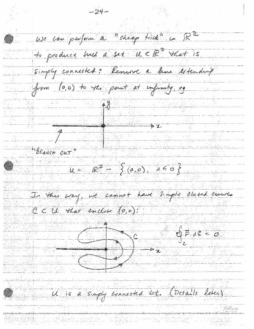
Let’s return to the idea of performing a line integration of what seems to be a gradient or conservative

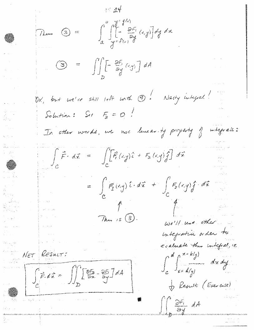
field F over a simple closed curve C. It may well be the case that the result in Eq. (105) is not correct,

i.e., a nonzero result is achieved. This does not imply that that FTLI 1 stated earlier is incorrect.

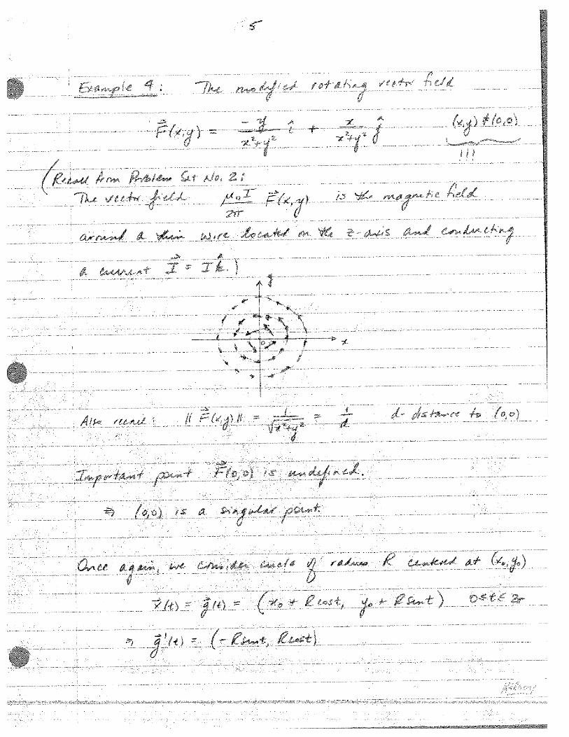
What may be happening is that the conditions of the theorem are not being satisfied. Many vector

fields in Physics have singularities, that is, points at which the fields are perhaps not defined, or not

continuous, or differentiable. For example, the electrostatic field E(r) produced by a point charge Q

situated at the origin,

E(r) =Q

4πǫ0r3r, (110)

where r = (x, y, z) and r = ‖r‖, is undefined at (0, 0, 0), the location of the point charge Q. (Part

of the problem is that the idea of a “point charge” is a mathematical idealization – in nature, there

really is no such thing as a “point charge” where a nonzero amount of electrical charge is situated at a

single point of zero volume. Even in the case of an electron, its charge is “smeared out.” Nevertheless,

it is often convenient to work with such idealizations and still come up with correct answers.)

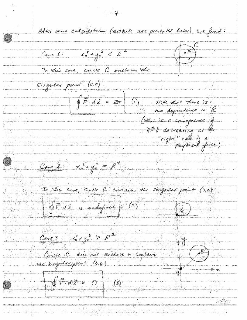
In such cases, a physical vector field F may actually be conservative except at its singular points.

For this reason, the region D over which line integrals (and later, surface integrals) involving F are

performed will have to be restricted in order to be able to guarantee that line integrals of F over all

simple closed curves in D are zero.

26

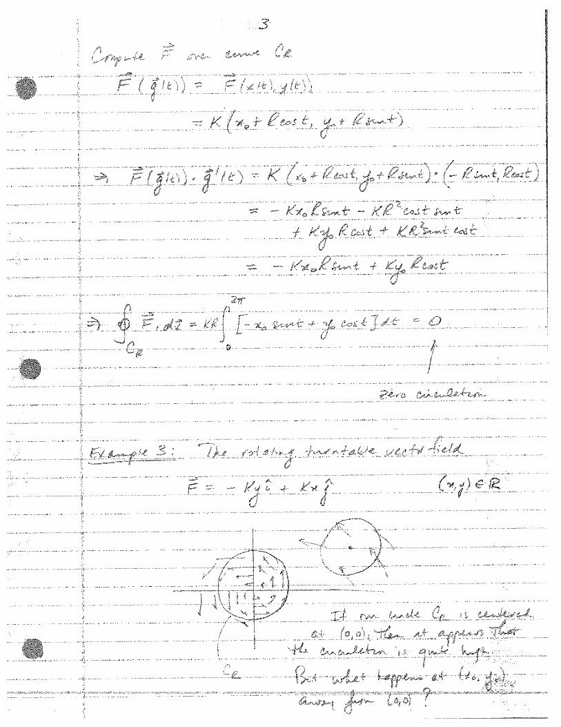
Circulation of a vector field around a closed curve C in R2

In this section, we consider the line integral of a planar vector field F around a simple closed curve C

in R2, denoted as∮

CF · dx . (111)

The convention is that the integration along C is performed in the counterclockwise direction so that

the region D enclosed by C lies always to the left of C as we move along the curve.

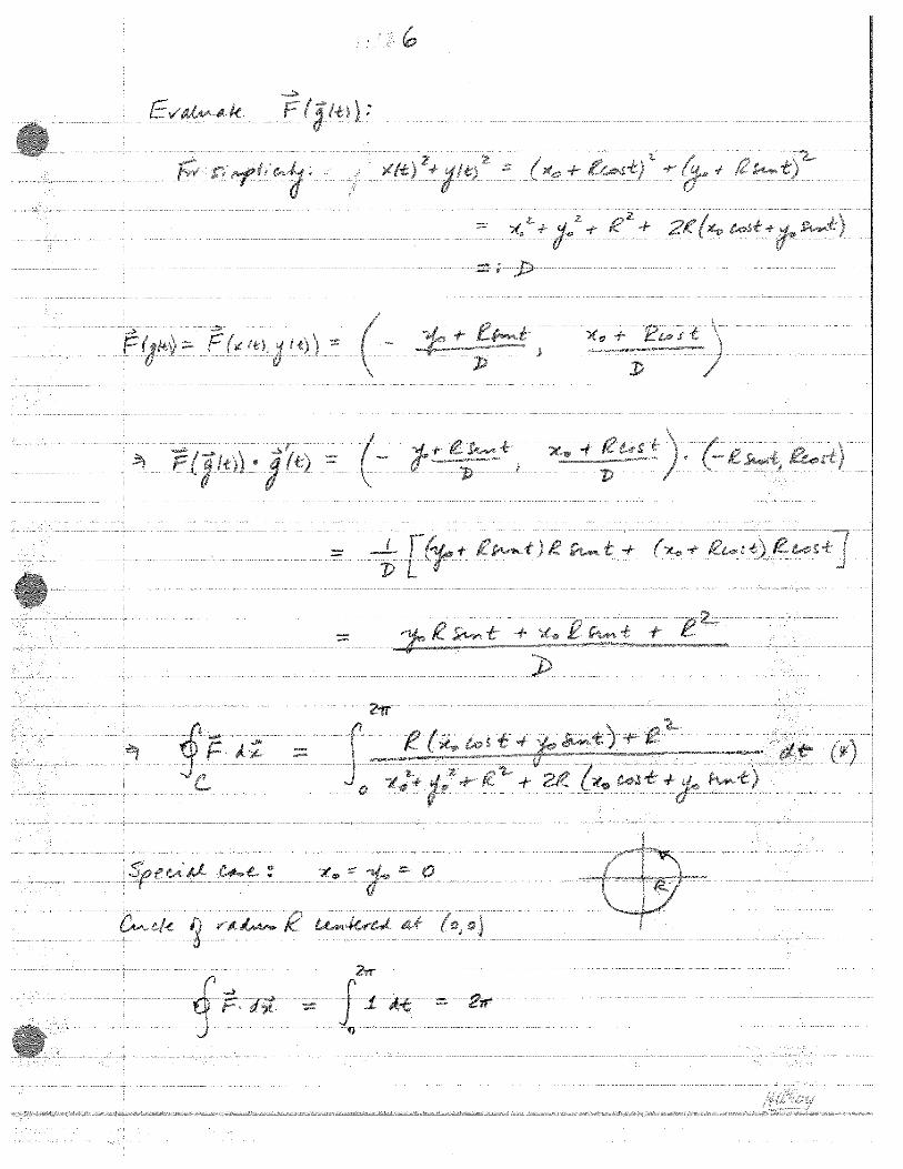
Assuming that we can parametrize the closed curve C as x(t) = g(t), a ≤ t ≤ b, with g(a) = g(b),

the line integral is normally computed as follows,

∮

CF · dx =

∫ b

aF(g(t))) · g′(t) dt (112)

We’ll perform a few practical computations shortly. At this time, however, let us make a few modifi-

cations to the above equation in order to discover some deeper meaning of this line integral:

∮

CF · ds =

∫ b

aF(g(t)) · g′(t) dt (113)

=

∫ b

aF(g(t)) ·

g′(t)

‖ g′(t) ‖‖ g′(t) ‖ dt

=

∫ b

aF(g(t)) · T̂(t) ds

=

∮

fds,

where the scalar-valued function,

f(g(t)) = F(g(t)) · T̂(t) , (114)

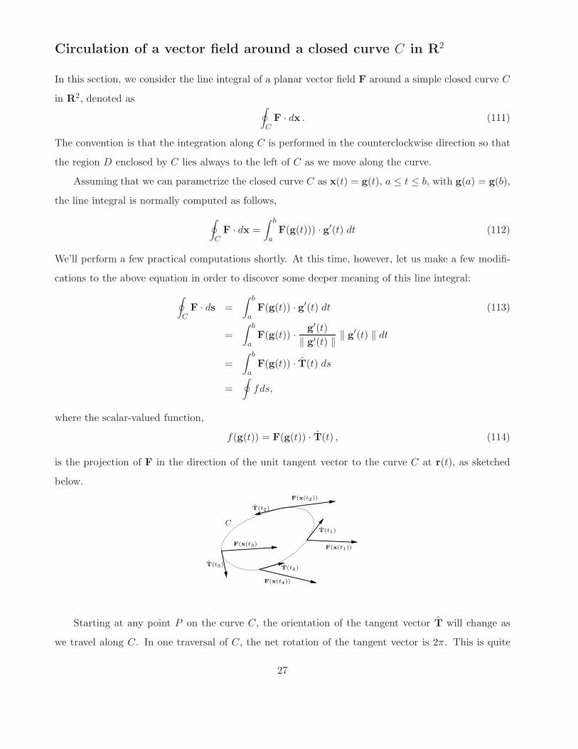
is the projection of F in the direction of the unit tangent vector to the curve C at r(t), as sketched

below.

CT̂(t1)

T̂(t2)

T̂(t3)

F(x(t3)

T̂(t4)

F(x(t4))

F(x(t1))

F(x(t2))

Starting at any point P on the curve C, the orientation of the tangent vector T̂ will change as

we travel along C. In one traversal of C, the net rotation of the tangent vector is 2π. This is quite

27

clear when C is a circle. The line integral in (113) sums up the projection of the vector field F(g(t))

onto the unit tangent vector T̂(t) to the curve. As such, we say that the line integral in (113) is the

circulation of the vector field F around the closed curve C.

If the vector field F is roughly parallel over the region D enclosed by curve C, then we expect the

line integral to be small in value – in some regions of the curve, F points in the same direction as T̂

and in others, it points in the opposite direction. In other words, the vector field exhibits very little

circulation.

28