Lecture 1: Review of Quantum Mechanics - Stanford Universitysporadic.stanford.edu/Math263C/lecture1.pdf · Lecture 1: Review of Quantum Mechanics Daniel Bump January 1, 2020. Operators

Operators on Hilbert space Quantum Mechanics The path integral

Lecture 1: Review of Quantum Mechanics

Daniel Bump

January 1, 2020


Hermitian (self-adjoint) operators on a Hilbert space are a keyconcept in QM.

In classical mechanics, an observable is a real-valued quantitythat may be measured from a system. Examples are position,momentum, energy, angular momentum.

In QM, a state of the system is a vector in a Hilbert space.Every classical observable A has a QM counterpart A that is aHermitian (self-adjoint) operator. Before discussing QM wediscuss operators.


Hermitian operators

If H is a Hilbert space, a bounded operator T is anendomorphism of H such that |T(v)| 6 c|v| for some constant c.The minimum value of c is the norm |T |.

If y ∈ H the functional x→ 〈Tx, y〉 is bounded, i.e. there is aconstant c with 〈Tx, y〉 6 c|x|. (c=|T | will work.) By the Rieszrepresentation theorem there exists T†y such that

〈Tx, y〉 = 〈x,T†y〉.

Then T† is the adjoint of T. If T = T† then T is called Hermitian(or self-adjoint).


Unbounded operators

We will also encounter unbounded operators on a Hilbert spaceH. An unbounded operator T is defined on a dense linearsubspace D ⊂ H.

LetD† = {y ∈ H|x 7→ (Tx, y) is bounded on D} .

The adjoint T† is then defined on D† by

(Tx, y) = (x,T†y).

Since D is dense, T†y is uniquely determined. T is symmetric ifD ⊆ D∗ and T∗ = T on D. Thus

(Tx, y) = (x,Ty), x, y ∈ D.

Then T is Hermitian if D∗ = D and T∗ = T.


Spectral theorem

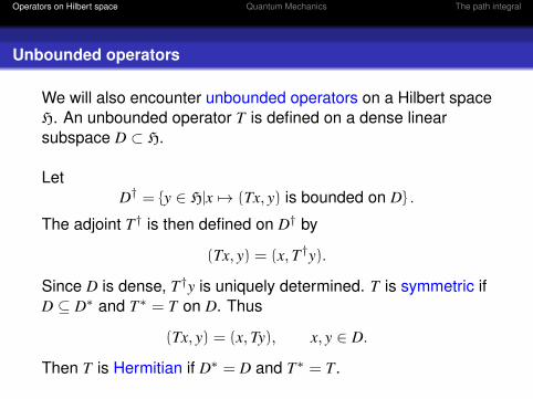
Let T : D→ H be an unbounded Hermitian operator. Thespectrum T is the set of λ ∈ C such that λI − T does not have abounded inverse. This implies that λ is real.

If T is a Hermitian unbounded operator, then there is a spectraltheorem. First assume that the spectrum is discrete. Let λi bethe eigenvalues of T. Then if v is in the spectrum, it is aneigenvector. Thus when the spectrum is discrete the spectrumis the set {λi} of eigenvalues. The spectral theorem in this caseasserts that every v ∈ H has an eigenvector expansion:

v =∑

i

vi, Tvi = λivi.

If the spectrum is not assumed discrete, there is still a spectraltheorem but we will not formulate it.


Self-adjoint extensions

The spectral theorem applies to self-adjoint operators, notsymmetric operators. So it is worth noting that every symmetricoperator has a self-adjoint extension. That is, we can enlargethe domain D to obtain a Hermitian operator.

Many operators can be defined with domain the Schwartzspace S(R) consisting of functions f such that f and all itsderivatives f (n) are of faster than polynomial decay. S(R) has atopology as a Frechet space, and a continuous linear functionalis called a tempered distribution.


Continuous spectrum: position and momentum

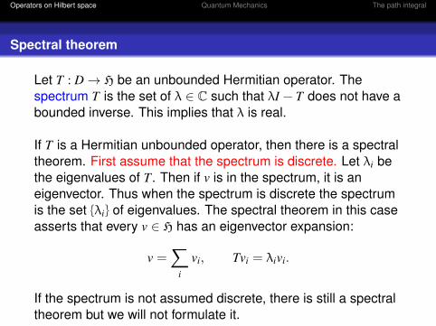
We consider the following unbounded operators on H = L2(R).Both will have domain initially S(R).

qf (x) = xf (x), pf (x) = −i hf ′(x).

These are symmetric operators. For q, this is easy. for p, itfollows by integration by parts: if f1 and f2 are Schwartzfunctions then

(pf1, f2) = −i h∫∞−∞ f ′1 (x)f2(x) dx = i h

∫∞−∞ f1(x)f ′2 (x) dx = (f1, pf2).

The spectrum of both q (position)and p (momentum) are all ofR, and they have no eigenvectors in H. However they haveeigenfunctions in the space of tempered distributions: δ(x − a)for q, and eiax for p.


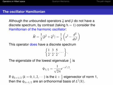
The oscillator Hamiltonian

Although the unbounded operators q and p do not have adiscrete spectrum, by contrast (taking h = 1) consider theHamiltonian of the harmonic oscillator:

H =12(p2 + q2) =

12

(x2 −

d2

dx2

)This operator does have a discrete spectrum{

12,

32,

52, · · ·}.

The eigenstate of the lowest eigenvalue 12 is

ψ1/2 =1√2π

e−x2/2.

If ψk+1/2 (k = 0, 1, 2, · · · ) is the k + 12 -eigenvector of norm 1,

then the ψk+1/2 are an orthonormal basis of L2(R).


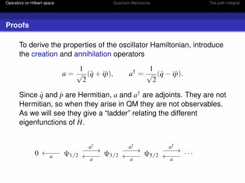
Proofs

To derive the properties of the oscillator Hamiltonian, introducethe creation and annihilation operators

a =1√2(q + ip), a† =

1√2(q − ip).

Since q and p are Hermitian, a and a† are adjoints. They are notHermitian, so when they arise in QM they are not observables.As we will see they give a “ladder” relating the differenteigenfunctions of H.

0 ψ1/2 ψ3/2 ψ5/2 · · ·a

a†

a

a†

a

a†

a


Proofs (continued)

Denote N = a†a. This is obviously self-adjoint and positivedefinite. Using [q, p] = i

[a, a†] = 1, H =12(aa† + a†a) = N +

12.

Since N is positive-definite, the spectrum of H is boundedbelow by 1

2 . We can exhibit one eigenfunction

ψ1/2(x) = π−1/4e−x2/2, Nψ1/2 = 0, Hψ1/2 =

12ψ1/2.


Proofs (continued)

The eigenfunctions of N must be nonnegative integers by thefollowing argument. We have

Na = a(N − 1)

which implies that if Nv = kv then Nav = (k − 1)av. Unless k is apositive integer, we may repeatedly apply a and obtain aneigenvector with negative eigenvalue, a contradiction since N ispositive definite.

On the other hand, using the identity

Na† = a†(N − 1)

applying a† increases the eigenvalue of N (or of H) by 1.


Proofs (continued)

We have(a†ψ, a†ψ) = (ψ,Nψ)

from which we see that the eigenfunctions

ψn+1/2(x) =1√n!(a†)nψ1/2

are orthonormal. In terms of the Hermite polynomials Hn wehave

ψn+1/2(x) =(√π2nn!

)−1/2 Hn(x)e−x2/2.

These are an orthonormal basis of L2(R). See Messiah,Quantum Mechanics Chapter XII and Appendix B.

(Note: there are different normalizations for Hermitepolynomials in the literature.)


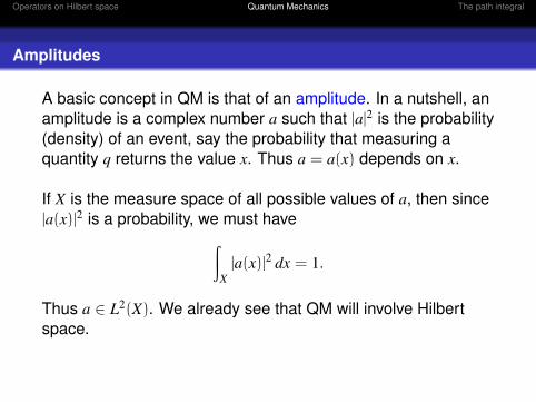
Amplitudes

A basic concept in QM is that of an amplitude. In a nutshell, anamplitude is a complex number a such that |a|2 is the probability(density) of an event, say the probability that measuring aquantity q returns the value x. Thus a = a(x) depends on x.

If X is the measure space of all possible values of a, then since|a(x)|2 is a probability, we must have∫

X|a(x)|2 dx = 1.

Thus a ∈ L2(X). We already see that QM will involve Hilbertspace.


Bra-Ket notation

The bra-ket notation was invented by Dirac. In mathematics it iscustomary for an inner product ( , ) to be linear in the firstcomponent and anti linear in the second. In physics theexpression 〈x|y〉 is linear in the second component andantilinear in the second. So

〈x|y〉 = (y, x).

If x ∈ H we denote |x〉 = x; in this notation |x〉 is called a ket.

Let H∗ be the Hilbert space dual of bounded linear functionalson H. As a real vector space it is isomorphic to H. Indeed theRiesz representation theorem asserts that every boundedlinear functional on H is of the form x 7→ (x, y) = 〈y|x〉 for somey ∈ H. Denote this functional 〈y| ∈ H∗. It is called a bra.


QM systems

A quantum mechanical system presupposes a Hilbert space H.A vector v of length 1 in H determines a state of the system.Note what happens to amplitudes when we multiply the vectorrepresenting the vector v by a complex number λ of absolutevalue 1. The amplitude a is replaced by λa but its probabilisticinterpretation that |a|2 is a probability (or probability density) isunchanged. Since all physical meaning of the state v is derivedfrom the amplitudes, the physical meaning of the state isunchanged.

Thus a state of the system is a ray in H, that is, aone-dimensional subspace. By the above all vectors of length 1in the ray have the same physical meaning, this is reasonable.


Classical limit

Quantum mechanics depends on a quantity h, Planck’sconstant. Classical Mechanics, which in its simplest form isNewton’s law F = ma (force equals mass times acceleration) isthe limiting theory h→ 0. Since h is small compared to theobserver, the universe appears to the observer to obey the lawsof classical mechanics.

There is another parameter c that appears in both quantum andclassical mechanics. This is the speed of light. The limit c→∞is nonrelativistic (classical or quantum) mechanics. Our firstexamples will be nonrelativistic but ultimately one must findrelativistic formulations.


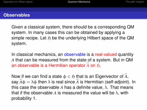
Observables

Given a classical system, there should be a corresponding QMsystem. In many cases this can be obtained by applying asimple recipe. Let H be the underlying Hilbert space of the QMsystem.

In classical mechanics, an observable is a real-valued quantityA that can be measured from the state of a system. But in QMan observable is a Hermitian operator A on H.

Now if we can find a state φ ∈ H that is an Eigenvector of A,say Aφ = λφ then λ is real since A is Hermitian (self-adjoint). Inthis case the observable A has a definite value, λ. That meansthat if the observable A is measured the value will be λ, withprobability 1.


Eigenfunction expansions

Let us consider the case where A has discrete spectrum. Thismeans that there is a sequence λ1 < λ2 < · · · of eigenvaluessuch that

H =⊕

Vλi

where Vi is the λi-eigenspace. Given a state φ we expandφ =

∑i aiφi where φi ∈ Vi. Then ai is the amplitude of

obtaining the value λi on measuring A, so |ai|2 is the probability

of this measurement. Note that∑|ai|

2 = |φ|2 = 1,

as required by this probabilistic interpretation.


Commuting operators

Suppose that A and B are observables whose correspondingoperator A and B commute. Then each A eigenspace isinvariant under B so the two operators can be simultaneouslydiagonalized. This means that H has a basis of elements thatare simultaneously eigenvectors for both operators, that is, forwhich both observables have definite values. The converse isalso obviously true: if such a basis exists then A and Bcommute.

In terms of measurements, this means that A and B commute ifand only if the observables A and B can be measuredsimultaneously. An example of operators that do not commuteare the angular momenta of a particle in two different directions.


The Hamiltonian

In classical mechanics, Emmy Noether proved thatcorresponding to every one-parameter subgroup of symmetriesof a physical system there is a corresponding conservedquantity, an observable. The observable corresponding tosymmetry under space translations, is momentum;corresponding to space rotations is angular momentum; andcorresponding to time translations is energy.

The QM observable corresponding to energy is the Hamiltonianoperator H. Let Ψ(t) be the state of the system at time t. Thetime evolution of the (nonrelativistic) system is given bySchrödinger’s equation

i h∂

dtΨ(t) = HΨ(t).


Eigenstates of the Hamiltonian

From Schrödinger’s equation,

i h∂

dtΨ(t) = HΨ(t) ,

if Ψ0 is an eigenstate of the Hamiltonian, say HΨ0 = EΨ0, wehave a stationary solution of the Hamiltonian with Ψ(0) = Ψ0:

Ψ(t) = ei hEtΨ0.

This is a solution with a definite energy E.

Assume that the Hamiltonian has a discrete spectrum. To bephysically realistic, should have a smallest eigenvalue λ0. Thecorresponding eigenstate (typically unique up to phase) iscalled the vacuum typically denoted |0〉 or |λ0〉.


Canonical quantization

A method of converting a classical system to a QM one is asfollows. Consider particles moving in Rd. Suppose thatxi = (x1

i , · · · , xdi ) (i = 1, · · · ,N) are the positions of the particles

of mass mi and pi are the corresponding momenta. These areall observables. Consider the Hilbert space H = L2(RNd), wherexj

i are the coordinate functions on RNd). The operators qji and pj

iare unbounded operators, defined on the Schwartz spaceS(RNd) of smooth functions f that are, with all their derivatives,of faster-than-polynomial decay.

The i-th position operator qji multiplies f ∈ S(RNd) by the (i, j)-th

coordinate function. And the i-th momentum operator

pji = −i h

∂

∂xji

.


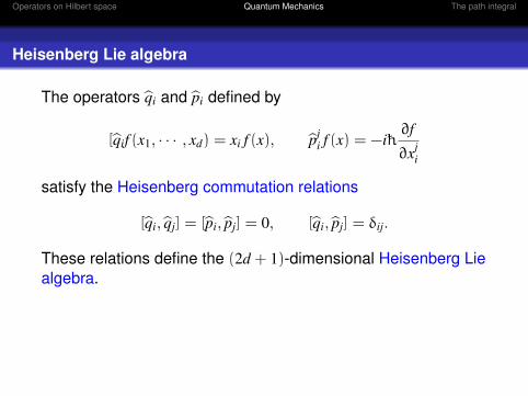
Heisenberg Lie algebra

The operators qi and pi defined by

[qif (x1, · · · , xd) = xi f (x), pji f (x) = −i h

∂f

∂xji

satisfy the Heisenberg commutation relations

[qi, qj] = [pi, pj] = 0, [qi, pj] = δij.

These relations define the (2d + 1)-dimensional Heisenberg Liealgebra.


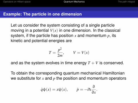
Example: The particle in one dimension

Let us consider the system consisting of a single particlemoving in a potential V(x) in one dimension. In the classicalsystem, if the particle has position x and momentum p, itskinetic and potential energies are

T =p2

2m, V = V(x)

and as the system evolves in time energy T + V is conserved.

To obtain the corresponding quantum mechanical Hamiltonianwe substitute for x and p the position and momentum operators

qψ(x) = xψ(x), p = −i h∂

∂x.


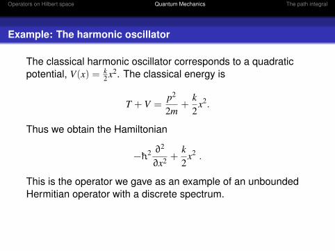
Example: The harmonic oscillator

The classical harmonic oscillator corresponds to a quadraticpotential, V(x) = k

2 x2. The classical energy is

T + V =p2

2m+

k2

x2.

Thus we obtain the Hamiltonian

− h2 ∂2

∂x2 +k2

x2 .

This is the operator we gave as an example of an unboundedHermitian operator with a discrete spectrum.


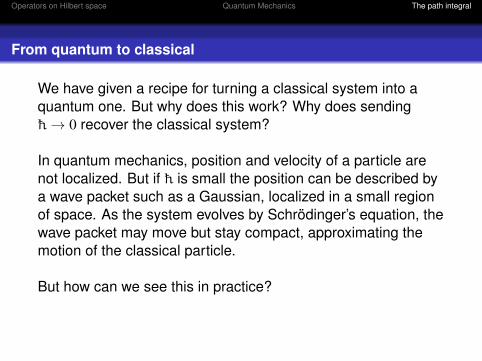
From quantum to classical

We have given a recipe for turning a classical system into aquantum one. But why does this work? Why does sending h→ 0 recover the classical system?

In quantum mechanics, position and velocity of a particle arenot localized. But if h is small the position can be described bya wave packet such as a Gaussian, localized in a small regionof space. As the system evolves by Schrödinger’s equation, thewave packet may move but stay compact, approximating themotion of the classical particle.

But how can we see this in practice?


The path integral

The path integral formulation of quantum mechanics originatedin Feynman’s dissertation, though it may have been understoodearlier by Dirac. It has advantages:

It easily gives relativistic formulationsIt works well in quantum field theory

Roughly a particle moves from an initial state to a final state. Tocalculate the amplitude of this process, one sums theamplitudes for every possible path.


The slit experiment

Lightsource

barrier screen

In the two-slit experiment particles (photons or massiveparticles such as electrons or atoms) are fired towards a barriercontaining two slits. A diffraction pattern appears.


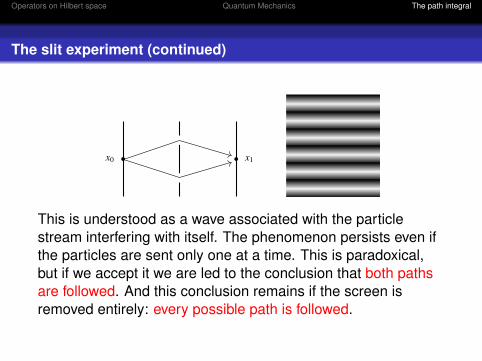
The slit experiment (continued)

x0 x1

This is understood as a wave associated with the particlestream interfering with itself. The phenomenon persists even ifthe particles are sent only one at a time. This is paradoxical,but if we accept it we are led to the conclusion that both pathsare followed. And this conclusion remains if the screen isremoved entirely: every possible path is followed.


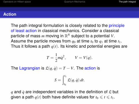
Action

The path integral formulation is closely related to the principleof least action in classical mechanics. Consider a classicalparticle of mass m moving in RN subject to a potential V.Assume the particle moves from q0 at time t0 to q1 at time t1.Thus it follows a path q(t). Its kinetic and potential energies are

T =12

mq2, V = V(q).

The Lagrangian is L(q, q) = T − V. The action is

S =

∫ t1

t0L(q, q) dt.

q and q are independent variables in the definition of L butgiven a path q(t) both have definite values for t0 6 t 6 t1.


About q

The meaning of q in these formulas depends on context.

In the definition of the Lagrangian,

L(q, q) =m2

q2 − V(q)

q is an independent variable. But when q(t) is a parametrizedpath, as in the definition of action:

S =

∫ t1

t0L(q, q) dt,

the parameter q has a definite value for all t, namely

q(t) =dqdt

(t).


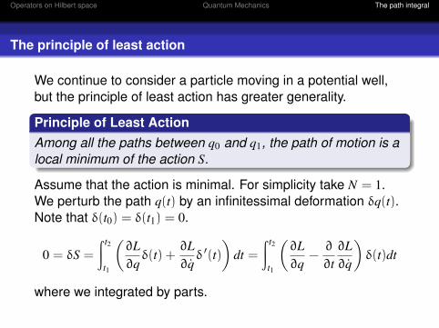
The principle of least action

We continue to consider a particle moving in a potential well,but the principle of least action has greater generality.

Principle of Least ActionAmong all the paths between q0 and q1, the path of motion is alocal minimum of the action S.

Assume that the action is minimal. For simplicity take N = 1.We perturb the path q(t) by an infinitessimal deformation δq(t).Note that δ(t0) = δ(t1) = 0.

0 = δS =

∫ t2

t1

(∂L∂qδ(t) +

∂L∂qδ ′(t)

)dt =

∫ t2

t1

(∂L∂q

−∂

∂t∂L∂q

)δ(t)dt

where we integrated by parts.


Euler Lagrange equations

Thus we obtain the Euler-Lagrange equation:

∂L∂q

−∂

∂t∂L∂q

= 0.

Let us check that these give the right equations of motion for aparticle in a potential well. In this case

∂L∂q

= −V ′(q) = force on the particle ,

∂L∂q

=∂

∂qT =

∂

∂q12

mq2 = mq,∂

∂t∂L∂q

= mq

so the Euler Lagrange equation boils down to:

“ Force equals mass times acceleration.”


From classical to quantum

We have considered the classical system of a particle movingin a potential V on RN . A state of the classical system assignsvalues in RN to q and q, positition and velocity. The subsequentevolution of the system as a function of t is then determined bythe Euler-Lagrange equations.

The analog in nonrelativistic quantum mechanics depends on aHilbert space H which we can take to be L2(RN). A state of thesystem is a one-dimensional subspace, represented by avector ψ. We normalize ψ so its L2 norm 〈ψ|ψ〉 = 1. Multiplyingψ by a phase factor eiθ does not change its physical meaning.


Review: Amplitudes

To reiterate a unit vector in the Hilbert space H = L2(RN)represents a state of the system consisting of a single particlein RN . The inner product is written

〈ψ1|ψ2〉 =∫RNψ1(x)ψ2(x) dx.

The precise location of the particle is not determined by ψ.Instead, the probability density of the particle being at the pointx is |ψ(x)|2. The value ψ(x) is called an amplitude.

More generally an amplitude is a complex number whose normsquare has interpretation as a probability or probability density.


Position versus momentum

The relation between the quantum and classical systems iscontrolled by a positive number h. The classical systememerges when h −→ 0.

The momentum similarly has a wave function φ which is theFourier transform of ψ :

φ(p) =1

(2π h)N/2

∫RNψ(q)e−ip·q/ hdq.

The Fourier transform is an isometry L2(RN) −→ L2(RN) so wemay regard either ψ or φ as a vector in an abstract Hilbertspace H. The position and momentum realizations of H maybe thought of different views of the same system.


Hermitian operators and the spectral theorem

A bounded operator T : H→ H is Hermitian or self-adjoint if

〈Tψ1|ψ2〉 = 〈ψ1|Tψ2〉.

In this case we use the notation 〈ψ1|T |ψ2〉.

TheoremT is compact and Hermitian, then H decomposes into theeigenspaces of T, which are all finite-dimensional (exceptperhaps the 0-eigenspace) and orthogonal.

We also encounter unbounded operators, defined on a densesubspace. There is a spectral theorem for unboundedHermitian operators.


Review: Observables

An observable is a quantity A such as position, momentum,energy, or angular momentum that can be measured from aphysical system.

In a quantum system the observable A corresponds to aHermitian operator A. If ψ is an eigenfunction then itseigenvalue λ is the measured value of A. If ψ is not aneigenfunction then measuring A does not have a deterministicoutcome. Two observables can be measured simultaneously ifand only if their operators commute.

The operator H corresponding to energy is called theHamiltonian.


Review:: The particle in one dimension

Let us consider the system consisting of a single particlemoving in a potential V(x) in one dimension. Position becomesthe unbounded operator q which is multiplication by x:

qψ(x) = xψ(x).

The momentum operator is

p = −i h∂

∂x

and we have the Heisenberg commutation relation [x, p] = i h.The operator corresponding to the classical energyE = T + V = p2

2m + V(x) is the Hamiltonian

H = − h2

2m∂2

∂x2 + V(x).


Review: The Hamiltonian as an evolution operator

In nonrelativistic quantum mechanics the Hamiltonian is anevolution operator.

A system prepared in state ψ0 at time t = t0 evolves accordingto Schrödinger’s equation. Let Ψ(x, t) be the state at time t soψ(x) = Ψ(x, t0).

i h∂

dtΨ(x, t) = HΨ(x, t). (1)

Schrödinger’s equation describes the evolution of ψ. Thus thestate ψ1(q) = Ψ(q, t1) at a later time t1 is

ψ1 = U(t1, t0)ψ0, U(t1, t0) = ei h(t1−t2)H.


The propagator amplitude as a Green’s function

Suppose the particle is prepared to be at location q0 at time t0and is found to be at q0 at time t1. The amplitude for thisprocess is an amplitude 〈q1|U(t1, t0)|q0〉. This propagator can beunderstood as a kernel

K(q1, t1, q0, t0) = 〈q1|U(t1, t0)|q0〉

for propogating solutions of the (nonrelativistic) Schrödingerequation. It is itself a solution (in either x0 or x1 and has a mildsingularity when x0 and x1 coincide.

Intuitively 〈q1|U(t1, t0)|q0〉 is the amplitude of the process, thatthe particle moves from x0 to x1.


The path integral

So what is this amplitude? According to Feynman, it is a pathintegral. For every possible path x(t) from x0 = (q0, t0) tox1 = (q1, t1) there is an action

S(x(t)) =∫ t1

t0L(q, q) dt

where L is the Lagrangian. According to the path integralformulation of quantum mechanics there is a measure [dx] onthe space of all possible paths x(t) from x0 to x1 such that:

〈q1|U(t1, t0)|q0〉 =∫

exp( i h

S(x(t)))[dx]


The wandering particle

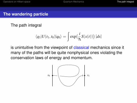
The path integral

〈q1|U(t1, t0)|q0〉 =∫

exp( i h

S(x(t)))[dx]

is unintuitive from the viewpoint of classical mechanics since itmany of the paths will be quite nonphysical ones violating theconservation laws of energy and momentum.

x0 x1


Stationary phase

Now let us recall the principle of stationary phase. This saysthat that given an oscillatory integral the main contribution tothe integral is where the oscillations are least. For exampleconsider ∫ b

aeiλφ(x) f (x)dx.

Suppose that there is a unique c ∈ (a, b) where φ ′(x) = 0, andφ ′′(c) > 0. Then if λ is large, the integral is approximately

eiλφ(c)f (c)

√2π

λφ ′′(c)eiπ/4.


Classical limit

Another manifestation of stationary phase is that if h is small,the main contribution to the path integral

〈q1|U(t1, t0)|q0〉 =∫

exp( i h

S(x(t)))[dx]

is from the classical path of least action, that is, from the pathx(t) that minimizes the action.

References for the path integral.

Polchinski, String Theory Vol.1, Appendix A: a short coursein path integralsDiFrancesco, Senechal and Mathieu, Conformal FieldTheory, Chapter 2Zee, Quantum Field Theory in a Nutshell, Chapter I.2.

Lecture 1: Review of Quantum Mechanics - Stanford Universitysporadic.stanford.edu/Math263C/lecture1.pdf · Lecture 1: Review of Quantum Mechanics Daniel Bump January 1, 2020. Operators

Documents