Lecture 1: Linear Programming · PDF filex of values to the decision variables x in such a way that (i) ... ( 0) j = 1;:::;n xj are the variables of the problem, ... feasible solution:

Lecture 1:

Linear Programming Models

Readings: Chapter 1; Chapter 2, Sections 1&2

1

Optimization Problems

Managers, planners, scientists, etc., are repeatedly faced with

complex and dynamic systems which they have to manage or

control in order to realize certain goals. These systems have

the following properties in common:

decision variables representing the options and oper-

ating levels the decision-maker can control in order to

drive the behavior of the system;

constraints limiting the range of control the decision-

maker has on the decision variables;

an objective that measures how well the system is op-

erating with regard to the goals of the decision maker.

2

Mathematical Programs

Mathematical programs are simply the presentation of an

optimization problem in a mathematically precise form. The

general description of a mathematical program is of the form

(MP )

max

min

f (x)x ∈ X

where

• x is the set of decision variables, which can be repre-

sented by numerical values, sets, functions, etc.

• X represents the feasible region describing the con-

straints on the decision variables. Feasible regions are

usually described by giving equalities and inequali-

ties involving functions of the decision variables. Any

point x ∈ X is called a feasible solution to the prob-

lem.

• f represents the objective function, a function of the

variable values that one wishes to maximize or mini-

mize.

3

Solving Mathematical Programs

The goal of solving a mathematical program (MP ) is to find

an optimal solution to the problem, that is, an assignment

x∗ of values to the decision variables x in such a way that

(i) x∗ is feasible to (MP );

(ii) x∗ has the “best” objective function value for (MP ) in

the sense that any other feasible solution x to (MP ) has

f (x) ≤ f (x∗) (for a max problem)

f (x) ≥ f (x∗) (for a min problem)

Questions Associated with Solving Mathematical

Programs:

• What are properties of the feasible region X , and its de-

scription, that help us in finding feasible and optimal so-

lutions to (MP )?

• What conditions can we give to show that a given solution

x is optimal to (MP )?

• What computational methods are available to find feasi-

ble and optimal solutions to (MP )?

• What is the relationship between the parameters describ-

ing (MP ) and the associated optimal solutions? How

sensitive are the solutions to the accuracy of the descrip-

tion of (MP )?

4

Woody’s Problem:

A Resource Allocation Model

Woody’s Furniture Company makes chairs and tables. Chairs

are made entirely out of pine, and require 8 linear feet of pine

per chair. Tables are made of pine and mahogany, with tables

requiring 12 linear feet of pine and 15 linear feet of mahogany.

Chairs require 3 hours of labor to produce and tables require

6 hours of labor. Chairs provide $35 profit and tables provide

$60 profit.

Woody has 120 linear feet of pine and 60 linear feet of

mahogany delivered each day, and has a work force of 6 car-

penters each of whom put in an 8-hour day. How should

Woody use his resources to provide the largest daily profits?

The mathematical program:

x1 = chairs per day, x2 = tables per day,

max z = 35x1 + 60x2 profits

8x1 + 12x2 ≤ 120 pine

15x2 ≤ 60 mahogany

3x1 + 6x2 ≤ 48 labor

x1 ≥ 0 x2 ≥ 0 nonnegativity

constraints

5

Linear Programming Models

Each of the models above are examples of linear programs.

Linear programs are characterized by the following proper-

ties:

optimization problem/mathematical program:

The problem involves finding the best value for a given

objective, subject to a given set of constraints.

deterministic: The behavior of the model is completely

determined, that is, there is no probability con-

tributing to the objective or constraints.

proportionality: Each variable contributes in direct

proportion to its value.

additivity: The variables in the objective and each con-

straint contribute the sum of the contributions of each

variable.

divisibility: The variables can take on continuous val-

ues subject to the constraints.

Any function satisfying the proportionality and additivity

properties is called a linear function, and will always have

the form

f (x1, . . . , xn) = a1x1 + . . . + anxn( + d).

6

Examples of Situations violating the LP

Assumptions

nonproportionality: fixed charges or volume discount-

ing (“$2000 to set the printer up, and $.15 per each

copy made”, “$100 for the first 50 copies, $1 for each

copy thereafter”)

nonadditivity: distances from a point (x, y) in the plane

to given point (a, b):√(x− a)2 + (y − b)2

(this is nonproportional as well). Volumes and square

footage (in terms of dimension) are also nonadditive (but

are proportional).

nondivisibility: integer/binary programs (“How many

aircraft to be made?”, “Should a new plant be built or

not?”, “must be made in lots of 5”)

7

The Mathematical Description

max

min

z = c1x1 + c2x2 + . . . + cnxn

ai1x1 + ai2x2 + . . . + ainxn

≤=

≥

bi i = 1, . . . ,m

xj

≥ 0

unrestricted,

(≤ 0)

j = 1, . . . , n

xj are the variables of the problem, and are allowed to

take on any set of real values that satisfy the constraints.

cj, bi, and aij are parameters of the problem, and (along

with dimensions n,m, and objective/row/variable types)

provide the precise description of a particular instance

of the LP model that you wish to solve.

cj are the objective/cost/profit coefficients.

bi are the right-hand-side/resource/demand coeffi-

cients.

aij are the proportionality/production/activity co-

efficients or coefficients of variation.

8

LP forms

There are several specific LP forms that will useful for vari-

ous purposes. The first is the standard (equality form)

max LP:

max z = c1x1 + c2x2 + . . . + cnxna11x1 + a12x2 + . . . + a1nxn = b1a21x1 + a22x2 + . . . + a2nxn = b2

... ...

am1x1 + am2x2 + . . . + amnxn = bmx1 ≥ 0 x2 ≥ 0 . . . xn ≥ 0.

Also useful is the inequality max LP:

max z = c1x1 + c2x2 + . . . + cnxna11x1 + a12x2 + . . . + a1nxn ≤ b1a21x1 + a22x2 + . . . + a2nxn ≤ b2

... ...

am1x1 + am2x2 + . . . + amnxn ≤ bm

9

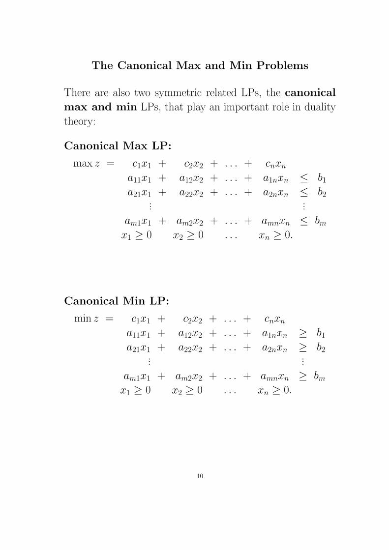
The Canonical Max and Min Problems

There are also two symmetric related LPs, the canonical

max and min LPs, that play an important role in duality

theory:

Canonical Max LP:

max z = c1x1 + c2x2 + . . . + cnxna11x1 + a12x2 + . . . + a1nxn ≤ b1a21x1 + a22x2 + . . . + a2nxn ≤ b2

... ...

am1x1 + am2x2 + . . . + amnxn ≤ bmx1 ≥ 0 x2 ≥ 0 . . . xn ≥ 0.

Canonical Min LP:

min z = c1x1 + c2x2 + . . . + cnxna11x1 + a12x2 + . . . + a1nxn ≥ b1a21x1 + a22x2 + . . . + a2nxn ≥ b2

... ...

am1x1 + am2x2 + . . . + amnxn ≥ bmx1 ≥ 0 x2 ≥ 0 . . . xn ≥ 0.

10

Definitions and Issues

feasible solution: A specific set of values of the vari-

ables that satisfy the constraints of that instance.

feasible region: The set of all feasible solutions for that

instance.

optimal solution: Any feasible solution whose objec-

tive function value is the greatest (for a max problem)

or smallest (for a min problem) of all points in the

feasible region.

Some issues:

• Does a particular instance of an LP have any feasible

point?

• Does the instance have an optimal solution?

• How can we describe the feasible region? What properties

does it have?

• How will we know that a solution to a particular instance

is in fact an optimal solution for that instance?

• Can we give an algorithm to find feasible/optimal solu-

tions for any instance of an LP, or to determine that none

exist for that instance?

• How efficient is that algorithm, particularly for solving

large LP instances?

11

A Graphical View of LPs

We can gain insight into the dynamics of LPs by looking at

2-variable problems. Consider Woody’s problem written in

inequality max form:

max z = 35x1 + 60x28x1 + 12x2 ≤ 120

15x2 ≤ 60

3x1 + 6x2 ≤ 48

−x1 ≤ 0

−x2 ≤ 0

Draw a picture of this LP, by performing the following steps:

1. Take each of the constraints (including the nonnegativity con-

straints), and draw the line describing the associated equal-

ity.

2. Determine which side of each equality line satisfies the in-

equality constraint. The feasible region is set of points which

lie on the correct side of all of the equality lines.

3. For particular objective function value z0, the isocost line

(or level set) at value z0 is described by the equality line

c1x1 + c2x2 = z0.

4. Slide this isocost line parallel and in the direction of im-

proving objective value until the last point at which it still

intersects the feasible region.

5. Any feasible point in this final intersection is an optimal so-

lution.

12

Example

max z = 35x1 + 60x2(C1) 8x1 + 12x2 ≤ 120

(C2) 15x2 ≤ 60

(C3) 3x1 + 6x2 ≤ 48

−x1 ≤ 0

−x2 ≤ 0

−2 0 2 4 6 8 10 12 14 16 18−3

−2

−1

0

1

2

3

4

5

6

7

x1

x2

C1

C2C3

13

Special subsets of the feasible region

interior: set of points having neighborhoods that lie en-

tirely in the feasible region. Equivalently, an interior

point is one that satisfies all inequalities strictly.

boundary: set of feasible points not in the interior, that

is, which satisfy one or more inequalities at equality

extreme point/corner point/vertex: boundary point

lying on n equalities, where n = the dimension of the

problem.

LP types

optimal solution: one can find a feasible solution for which

no other solution has a better objective function value.

infeasible LP: the constraints of the problem are such

that the feasible region is empty, in other words, there

is no feasible solution.

unbounded LP: (maximization problem) the objective and

constraints of the problem are such that there is no up-

per bound on the objective function values of the fea-

sible points. That is, for every feasible solution there ex-

ists another feasible solution with larger objective func-

tion value. (A symmetric definition applies for mini-

mization problems.)

14

Three Types of Linear Programs

Optimal Solution

max z = 35x1 + 60x2(C1) 8x1 + 12x2 ≤ 120

(C2) 15x2 ≤ 60

(C3) 3x1 + 6x2 ≤ 48

−x1 ≤ 0

−x2 ≤ 0

−2 0 2 4 6 8 10 12 14 16 18−3

−2

−1

0

1

2

3

4

5

6

7

x1

x2

C1

C2C3

15

Infeasible LP

max z = 35x1 + 60x2(C1) 8x1 + 12x2 ≥ 120

(C2) 15x2 ≥ 60

(C3) 3x1 + 6x2 ≤ 48

−x1 ≤ 0

−x2 ≤ 0

−2 0 2 4 6 8 10 12 14 16 18

−2

0

2

4

6

8

10

12

x1

x2

C1

C2

C3

16

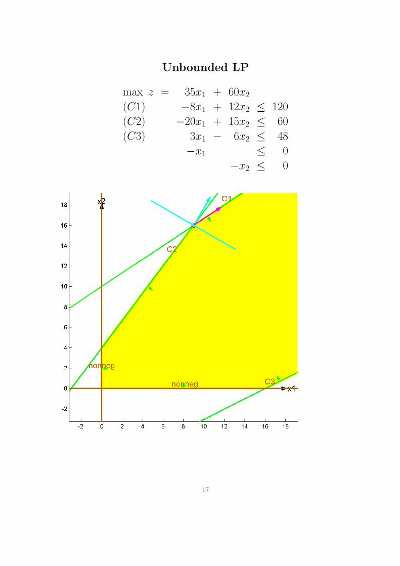
Unbounded LP

max z = 35x1 + 60x2(C1) −8x1 + 12x2 ≤ 120

(C2) −20x1 + 15x2 ≤ 60

(C3) 3x1 − 6x2 ≤ 48

−x1 ≤ 0

−x2 ≤ 0

17

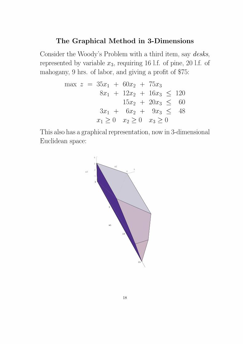
The Graphical Method in 3-Dimensions

Consider the Woody’s Problem with a third item, say desks,

represented by variable x3, requiring 16 l.f. of pine, 20 l.f. of

mahogany, 9 hrs. of labor, and giving a profit of $75:

max z = 35x1 + 60x2 + 75x38x1 + 12x2 + 16x3 ≤ 120

15x2 + 20x3 ≤ 60

3x1 + 6x2 + 9x3 ≤ 48

x1 ≥ 0 x2 ≥ 0 x3 ≥ 0

This also has a graphical representation, now in 3-dimensional

Euclidean space:

0

5

10

15

x1

01

23

45

x2

0

1

2

3

4

x3

5

10

15

x1

18

The level set is now a flat sheet perpendicular to the ob-

jective function vector (35,60,75). Adding this to the picture,

we get

0

5

10

15

chairs

-5

0

5 tables

-5

0

5

10

desks

0

5

10

15

chairs

We can slide this level set to the optimal solution (12,2,0),

although this is difficult to conceptualize even in 3 dimen-

sions, and becomes completely unwieldy in higher dimen-

sions.

19

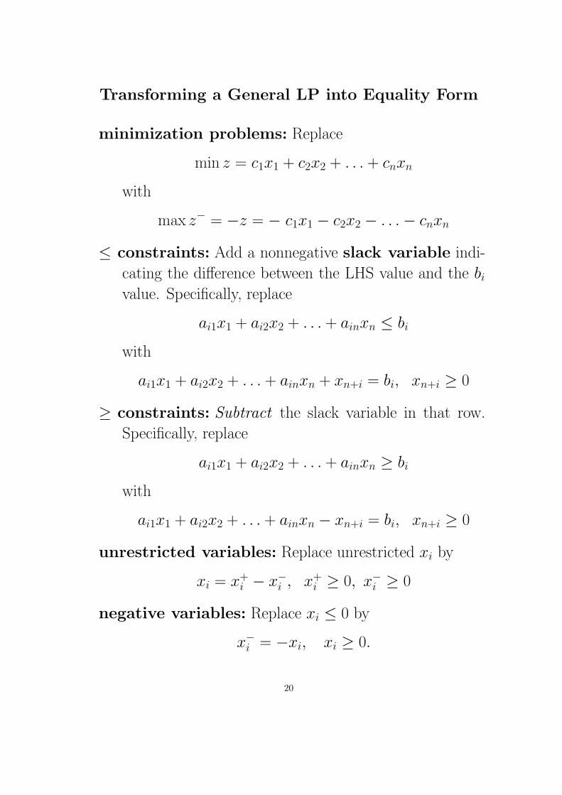
Transforming a General LP into Equality Form

minimization problems: Replace

min z = c1x1 + c2x2 + . . . + cnxn

with

max z− = −z = − c1x1 − c2x2 − . . .− cnxn

≤ constraints: Add a nonnegative slack variable indi-

cating the difference between the LHS value and the bivalue. Specifically, replace

ai1x1 + ai2x2 + . . . + ainxn ≤ bi

with

ai1x1 + ai2x2 + . . . + ainxn + xn+i = bi, xn+i ≥ 0

≥ constraints: Subtract the slack variable in that row.

Specifically, replace

ai1x1 + ai2x2 + . . . + ainxn ≥ bi

with

ai1x1 + ai2x2 + . . . + ainxn − xn+i = bi, xn+i ≥ 0

unrestricted variables: Replace unrestricted xi by

xi = x+i − x−i , x+i ≥ 0, x−i ≥ 0

negative variables: Replace xi ≤ 0 by

x−i = −xi, xi ≥ 0.

20

Examples

Woody’s problem can be put into standard max form by

simply adding slack variables to each of the inequalities

max z = 35x1 + 60x28x1 + 12x2 + x3 = 120

15x2 + x4 = 60

3x1 + 6x2 + x5 = 48

x1 ≥ 0 x2 ≥ 0 x3 ≥ 0 x4 ≥ 0 x5 ≥ 0

Now consider the following LP:

min z = 35x1 + 60x2−8x1 + 12x2 = 120

−20x1 + 15x2 ≥ 60

2x1 − 6x2 ≤ 48

x1 unrest. x2 ≤ 0

Here we subtract a slack in Row 2, add a slack in Row 3,

negate the objective function, replace x1 with x1 = x+1 − x−1and replace x2 by −x−2 to get standard max LP

max z− = −35x+1 + 35x−1 + 60x−2−8x+1 + 8x−1 − 12x−2 = 120

−20x+1 + 20x−1 − 15x−2 − x4 = 60

2x+1 − 2x−1 + 6x−2 + x5 = 48

x+1 ≥ 0 x−1 ≥ 0 x−2 ≥ 0 x4 ≥ 0 x5 ≥ 0

21

A Statistics Problem

You are given a set of sample points

(x1, y1), (x2, y2), . . . , (xn, yn),

which are suppose to satisfy a linear equation of the form

Y = aX + b. Due to experimental error, they do not simul-

taneously satisfy the same equation. You want to find the

“best” equation to fit to these sample points.

X

Y

(9,6)

(12,-1)(16,-2)

(3,7)

(6,2)

(3,10)

(9,7)

(14,3)

(18,1)

n=9

Y=aX+b

22

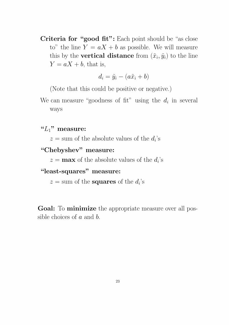
Criteria for “good fit”: Each point should be “as close

to” the line Y = aX + b as possible. We will measure

this by the vertical distance from (xi, yi) to the line

Y = aX + b, that is,

di = yi − (axi + b)

(Note that this could be positive or negative.)

We can measure “goodness of fit” using the di in several

ways

“L1” measure:

z = sum of the absolute values of the di’s

“Chebyshev” measure:

z = max of the absolute values of the di’s

“least-squares” measure:

z = sum of the squares of the di’s

Goal: To minimize the appropriate measure over all pos-

sible choices of a and b.

23

Formulating the LP for the L1 Measure

The optimization problem has as variables the two numbers

a and b describing the linear equation. Once we have these

numbers we can compute the di’s by adding the n equations

di = yi − (axi + b), i = 1, . . . , n. Note that while the x’s

and y’s are parameters, the di’s are now auxiliary vari-

ables.

The optimization problem can be stated mathematically as:

min z = |di| + |d2| + . . . + |dn|

di = yi − (axi + b), i = 1, . . . , n

a, b, di unrestricted

Although the constraints are linear, the objective function

is not.

24

Dealing with Unrestricted Variables

Each unrestricted variable is now separated into its positive

and negative parts:

a = a+ − a−

b = b+ − b−, and

di = d+i − d−i i = 1, . . . , n

Added bonus: The absolute value of di can be written

|di| = d+i + d−i .

Thus the objective function can be rewritten

min z = d+1 + d−1 + . . . + d+n + d−n

25

Formulating the LP for the Chebyshev Measure

The objective here is

min z = max{|di|, |d2|, . . . , |dn|}= max{d+1 + d−1 , . . . , d

+n + d−n }

Again, this is not linear. To formulate it as a linear program,

we introduce still another auxiliary variable M , restricting it

by the inequalities

M ≥ d+i + d−i , i = 1, . . . , n

or, in equality form,

d+i + d−i + si = M, i = 1, . . . , n

where the si’s are the slack variables. Minimizing z = M

subject to the above constraints will insure that M will in

fact take the value of the maximum of the |di|’s.

26

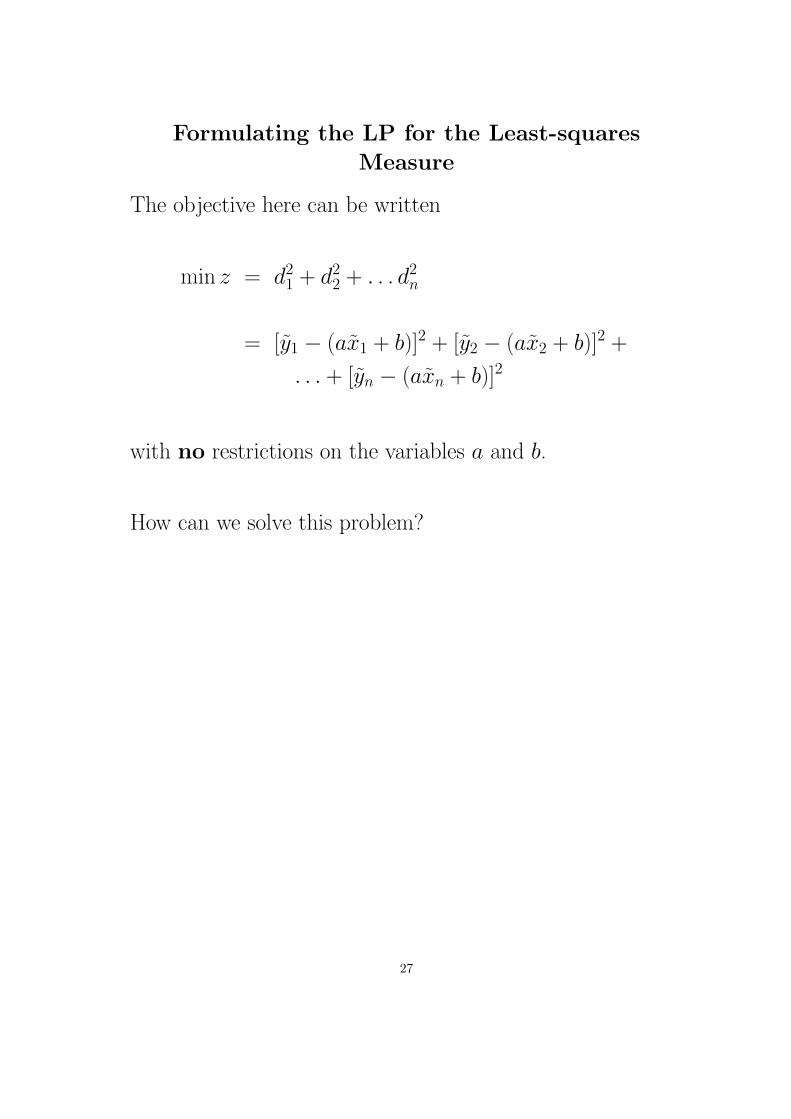
Formulating the LP for the Least-squares

Measure

The objective here can be written

min z = d21 + d22 + . . . d2n

= [y1 − (ax1 + b)]2 + [y2 − (ax2 + b)]2 +

. . . + [yn − (axn + b)]2

with no restrictions on the variables a and b.

How can we solve this problem?

27

Transforming a General LP into Canonical Form

We can also transform LPs into canonical max form. The

transformations for variable types are the same, and the

transformations for constraints are as follows:

≥ constraints: Simply negate the constraint.

Equality constraints: Replace the constraint

ai1x1 + ai2x2 + . . . + ainxn = bi

with the two constraints

ai1x1 + ai2x2 + . . . + ainxn ≤ bi

and

−ai1x1 − ai2x2 − . . .− ainxn ≤ −bi

Note that no slack variables are necessary for this trans-

formation.

Example: The general form LP given above has equivalent

canonical max form

max z− = −35x+1 + 35x−1 + 60x−2−8x+1 + 8x−1 − 12x−2 ≤ 120

+8x+1 − 8x−1 + 12x−2 ≤ −120

20x+1 − 20x−1 + 15x−2 ≤ −60

2x+1 − 2x−1 + 6x−2 ≤ 48

x+1 ≥ 0 x−1 ≥ 0 x−2 ≥ 0

28