Lecture 1: Introduction & Mathematical Modeling

Copyright ©1994-2012 by K. Pattipati

ECE 6095/4121

Digital Control of Mechatronic Systems

Lecture 1: Introduction &

Mathematical Modeling Prof. Krishna R. Pattipati

Prof. David L. Kleinman

Dept. of Electrical and Computer Engineering

University of Connecticut Contact: [email protected] (860) 486-2890

mailto:[email protected]

Copyright ©1994-2012 by K. Pattipati 2

Contact Information

– Room number: ITE 350

– Tel/Fax: (860) 486-2890/5585

– E-mail: [email protected]

Office Hours: Tuesday – Wednesday: 11:00-12:00 Noon

Very demanding course

– Homework every week and Design Projects (50%)

– Sensors and Actuators Presentation (10%)

– Class project (20%)

– Paper presentation (5%)

– Midterm – Take Home (15%)

Course Materials: http://huskyct.uconn.edu

Introduction

mailto:[email protected]

http://husyct.uconn.edu/




Background Needed

Expected Background Knowledge (ECE 5101, ECE3111)

• Differential equations

• Continuous-time system modeling methods

– Transfer functions, state-space models (canonical forms, minimal

realizations)

– Controllability & Observability

– Transient response, especially for 2nd-order systems

• Stability theory for continuous-time systems

– Feedback, Routh-Hurwitz, Lyapunov Theory

• Graphical Tools

– Bode plot, Nyquist plot, Nichols Chart, and Root-locus

• Some basic knowledge of discrete-time systems

– Z-transforms, difference equations, and signal sampling

• Matrix theory and Linear Algebra

• Knowledge and use of MATLAB


Mechatronic Systems Introduction & Overview

1. What is Mechatronics?

2. Elements of Mechatronics

3. Mechatronics Applications

4. Example of Mechatronics Systems

5. Mathematical Modeling of Mechatronic Systems

− Diesel Engine Driving a Pump

− Armature-controlled DC Motor

− Magnetic Levitation

− Inverted Pendulum

− Induction Motor Spray Painting in an Automotive Plant

6. Different Mathematical Representations of Systems


What is Mechatronics? - 1

• The term “Mechatronics" was first coined by Tetsuro Mori, a senior engineer of

the Japanese company Yasakawa*, in 1969

− T. Mori, “Mechatronics,” Yasakawa Internal Trademark Application Memo, 21.131.01, July 12,

1969.

− R. Comerford, “Mecha … what?” IEEE Spectrum, 31(8), 46-49, 1994.

• Mechatronics refers to electro-mechanical systems and is centered on mechanics,

electronics, computing and control which, when combined, make possible the

generation of simpler, more economical, reliable and versatile systems

• Mechatronics is the synergistic integration of mechanical engineering, electronics

and intelligent computer control in design and manufacture of products and

processes

− F. Harshama, M. Tomizuka, and T. Fukuda, “Mechatronics-what is it, why, and how?-and

editorial,” IEEE/ASME Trans. on Mechatronics, 1(1), 1-4, 1996.

• Synergistic use of precision engineering, control theory, computer science, and

sensor and actuator technology to design improved products and processes.”

– S. Ashley, “Getting a hold on mechatronics,” Mechanical Engineering, 119(5), 1997.

* Makes servos, machine controllers, AC motor drives, switches and robots

5


What is Mechatronics? - 2

• Field of study involving the analysis, design, synthesis, and selection of systems

that combine electronics and mechanical components with modern controls and

microprocessors.

− D. G. Alciatore and M. B. Histand, Introduction to Mechatronics and Measurement Systems, McGraw Hill, 1998.

− Good site for mechatronics: http://www.engr.colostate.edu/~dga/mechatronics/definitions.html

• Our working definition: Mechatronics is the synergistic integration of

sensors, actuators, signal conditioning, power electronics, decision and

control algorithms, and computer hardware and software to manage

complexity, uncertainty, and communication in engineered systems.

• An Embedded system, a component of mechatronics system, is a combination

of hardware and software designed to run on its own without human intervention,

and may be required to respond to events in real-time

• When these systems are networked, they are called Cyber-physical systems

− Numerous applications: Zero-accident highways, smart grid, smart buildings, tele-

operation rooms, aerospace and transportation, robotics and intelligent machines,…..

6

http://www.engr.colostate.edu/~dga/mechatronics/definitions.html













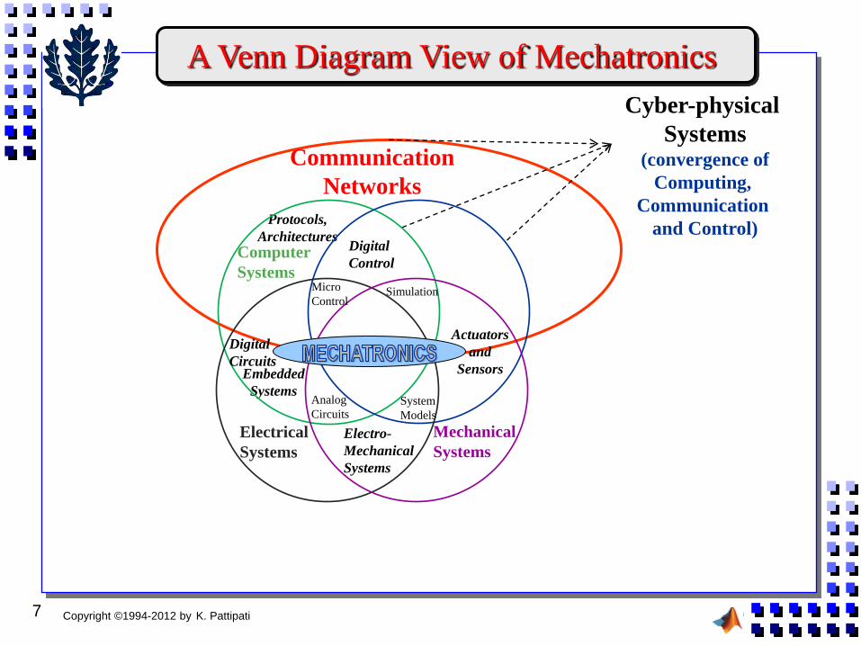
A Venn Diagram View of Mechatronics

Communication

Networks

Protocols,

Architectures

Cyber-physical

Systems (convergence of

Computing,

Communication

and Control)

Embedded

Systems

Computer

Systems Micro

Control Simulation

Analog

Circuits System

Models

Digital

Control

Electro-

Mechanical

Systems

Actuators

and

Sensors

Digital

Circuits

Electrical

Systems

Mechanical

Systems

7


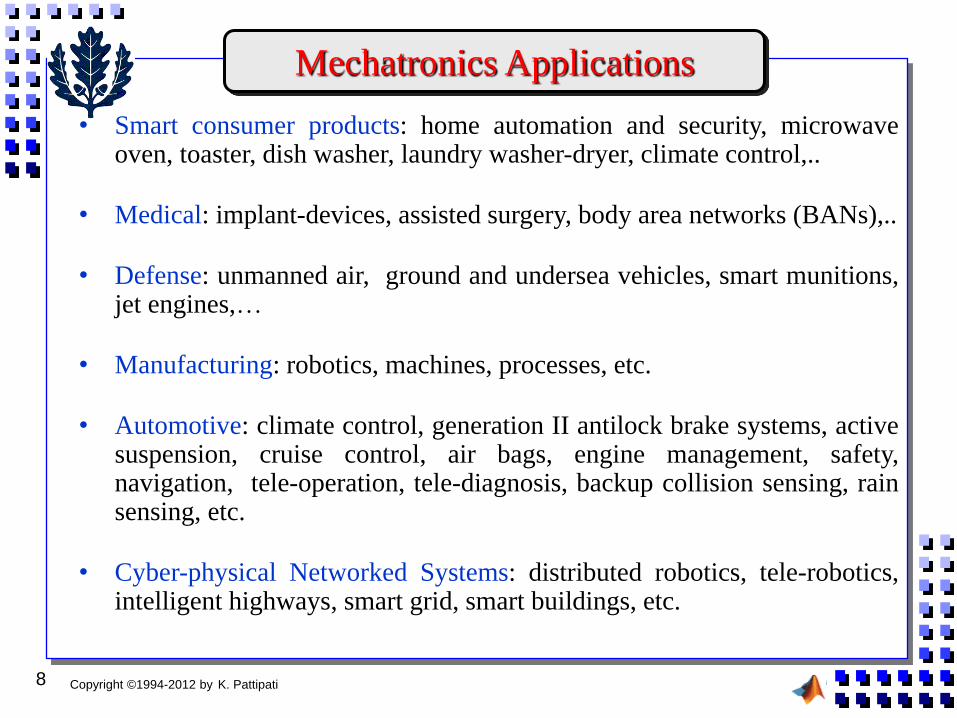
Mechatronics Applications

• Smart consumer products: home automation and security, microwave oven, toaster, dish washer, laundry washer-dryer, climate control,..

• Medical: implant-devices, assisted surgery, body area networks (BANs),..

• Defense: unmanned air, ground and undersea vehicles, smart munitions, jet engines,…

• Manufacturing: robotics, machines, processes, etc.

• Automotive: climate control, generation II antilock brake systems, active suspension, cruise control, air bags, engine management, safety, navigation, tele-operation, tele-diagnosis, backup collision sensing, rain sensing, etc.

• Cyber-physical Networked Systems: distributed robotics, tele-robotics, intelligent highways, smart grid, smart buildings, etc.

8


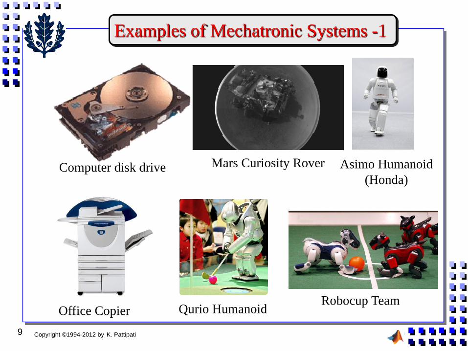
Examples of Mechatronic Systems -1

Computer disk drive Asimo Humanoid

(Honda)

Mars Curiosity Rover

Robocup Team Qurio Humanoid Office Copier

9

http://en.wikipedia.org/wiki/Image:Asimohonda.jpg


Examples of Mechatronic Systems -2

Aviation Underwater Robot Flying UAV

Big Dog Robot HEXAPOD Robot Micro Robot

10


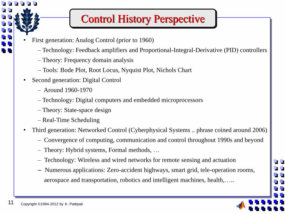
Control History Perspective

• First generation: Analog Control (prior to 1960)

– Technology: Feedback amplifiers and Proportional-Integral-Derivative (PID) controllers

– Theory: Frequency domain analysis

– Tools: Bode Plot, Root Locus, Nyquist Plot, Nichols Chart

• Second generation: Digital Control

– Around 1960-1970

– Technology: Digital computers and embedded microprocessors

– Theory: State-space design

– Real-Time Scheduling

• Third generation: Networked Control (Cyberphysical Systems .. phrase coined around 2006)

– Convergence of computing, communication and control throughout 1990s and beyond

– Theory: Hybrid systems, Formal methods, …

– Technology: Wireless and wired networks for remote sensing and actuation

– Numerous applications: Zero-accident highways, smart grid, tele-operation rooms,

aerospace and transportation, robotics and intelligent machines, health,…..

11


Feedback Control System

12

Adapted from

Astrom & Murray, 2011

• Process = actuators + dynamic system + sensors

• Noise and external disturbances perturb the dynamics of the process

• Controller = pre-filter + A/D + computer + D/A+ system clock

• Operator input = reference signal (set point, desired input)

Copyright © 1994-2012 by K. Pattipati 13

Control System Design Process

A) Mathematical Model of System (Process) to be Controlled

MATH MODEL OF SYSTEM

PERFORMANCE MEASURES

CONTROL

DESIGN

EVALUATION &

SIMULATION OK?

NO B

C

YES

A

B) Performance Measures and Concerns

Mathematical criteria that are driven by customer's qualitative/quantittaive specifications

for behavior of the closed-loop (feedback) system

(1) Stability of the closed-loop system

(2) Steady-state accuracy, Integral absolute error (IAE), integral square error (ISE)

(3) Speed of response/transient

(4) Sensitivity/robustness

C) Evaluation and Simulation

− Computer-aided Engineering (CAE) software tools such as MATLAB/Simulink,LabVIEW

− Hardware-in-the-loop simulation

Focus of the course

Copyright ©2012 by K.R. Pattipati 14

Relationships among LTI Modeling Techniques

Transfer Functions

G(s)

Ordinary Differential

Equations (ODE)

State Variables

Signal Flow Graphs

sdt

d

• Physical Variables

• Standard Controllable form (SCF)

• Standard Observable form (SOF)

• Modal (Diagonal) form

DuxCy

BuxAx

DBAsICsG 1)()(

SCF, SOF

Modal

LTI: Linear Time-invariant

Useful for

Nonlinear

Systems

as well

(SFG as Simulink

Diagram. Mason’s

Rule not applicable)


Math Modeling involves Diverse Disciplines - 1

• Classic Book

− R. H. Cannon. Dynamics of Physical Systems. Dover, 2003 or McGraw-Hill, 1967.

• Mechanics

− V. I. Arnold. Mathematical Methods in Classical Mechanics. Springer, 1978.

− H. Goldstein. Classical Mechanics. Addison-Wesley, Cambridge, MA, 1953.

• Thermal

− H. S. Carslaw and J. C. Jaeger. Conduction of Heat in Solids. Clarendon Press,1959.

• Fluids

− J. F. Blackburn, G. Reethof, and J. L. Shearer. Fluid Power Control. MIT Press,1960.

• Vehicles

− M. A. Abkowitz. Stability and Motion Control of Ocean Vehicles. MIT Press, 1969.

− J. H. Blakelock. Automatic Control of Aircraft and Missiles. Addison-Wesley, 1991.

− J. R. Ellis. Vehicle Handling Dynamics. Mechanical Engineering Pubs., London,1994.

− U. Kiencke and L. Nielsen. Automotive Control Systems: For Engine, Driveline, and

Vehicle. Springer, Berlin, 2000.


Math Modeling involves Diverse Disciplines - 2

• Robotics

− M. W. Spong & M. Vidyasagar, Dynamics and Control of Robot Manipulators. Wiley, ‘89.

− R. M. Murray, Z. Li, and S. S. Sastry. A Mathematical Introduction to Robotic

Manipulation. CRC Press, 1994.

• Power Systems

− P. Kundur. Power System Stability and Control. McGraw-Hill, New York, 1993.

• Acoustics

− L. L. Beranek. Acoustics. McGraw-Hill, New York, 1954.

• Micromechanical Systems

− S. D. Senturia. Microsystem Design. Kluwer, Boston, MA, 2001.

• Biological Systems

− J. D. Murray. Mathematical Biology, Vols. I and II. Springer-Verlag, 2004.

− H. R. Wilson. Spikes, Decisions, and Actions: The Dynamical Foundations of

Neuroscience. Oxford University Press, Oxford, UK, 1999.

Copyright © 2012 by K.R. Pattipati 17

Force-Voltage Analogy for Translational Systems

dt

diLV

dt

dvMMaf

RiVdt

dxBBvf

dticc

qVdtvktkxf

1)(

Key Mechanical Elements:

• spring

• viscous damper

• mass

K

)(tx

)(tf

B

)(tx

)(tf

x

fM 1

capacitor spring

resistor damper

inductor mass

current velocity

chargeposition

voltage force

CK

RB

LM

iv

qx

Vf

Analogy

spring

damper

mass


Torque-Voltage Analogy for Rotational Systems

J

K

B

u(t)

input torque

,

dt

diLVJJT

RiVBBT

dtiCC

qVdtKKT

1

Analogy

C/1Capacitor Spring

ResistorDamper

Inductor inertia ofMoment

Current Velocity

Chargent Displaceme

VoltageTorque

K

RB

LJ

i

q

VT

Damper

Torsion Spring


Diesel Engine Driving a Pump

K

1

Electrical Analog

1

1

1

1B

2BJT System Equations

KTB

KKT

haveweTB

ceAlso

KT

TJJ

B

BJKBT

pumplocity of Angular ve

Tthe springTorque in

States

1

1

1

1

2

2111

,1

sin,

)(

1

)()(

,

,

:

Ty

KTB

KK

JJ

B

T

01

0

1

1

2

Input:

Output:

Draw Signal Flow Graph and Compute Transfer Function,

Steady state gain? System type?

1

2

1

Alternate States:

( , ) ( , )x

BK x

J

Kx x

B


Analysis of Engine Driving a Pump

2

1

2

1

0 0.25 0.5 0

20 4 20

10 101 0 ( ) 3.32; 0.64;

4.25 11 11n

B

J J

KT T K T TK

B

y G s dc gainT s s

2 2

1

2

20 . / ;

2 . / ;

5 . .sec/ ;

0.5 . .sec/

K N m rad

J kg m rad

B N m rad

B N m rad

0 0.5 1 1.5 2 2.5 30

0.1

0.2

0.3

0.4

0.5

0.6

0.7

0.8

0.9

1

Step Response

Time (seconds)

Am

plit

ude

-60

-50

-40

-30

-20

-10

0

Magnitu

de (

dB

)

10-1

100

101

102

-180

-135

-90

-45

0

Phase (

deg)

Bode Diagram

Frequency (rad/s)

Copyright © 2012 by K.R. Pattipati

DC Motors

DC Motors convert DC energy into mechanical energy used in disk drives, robots, tape

transport mechanisms

Nice animation at:

− http://www.wisc-online.com/objects/ViewObject.aspx?ID=IAU13208



Torque of a DC motor:

− Field controlled: iA constant; iF controlled;

− Armature controlled: iF constant; iA controlled;

Three types of DC motors: series wound, shunt and compound

currentArmatureicurrentFieldiiKiT AFAFm ;;

FFm iKT

ATm iKT

21

http://www.wisc-online.com/objects/ViewObject.aspx?ID=IAU13208














Armature Controlled DC Motors (Fixed Field )

Fixed field is created by permanent magnets surrounding the armature

Applying an input voltage to the armature circuit causes a current in the coils of the

armature

This generates a magnetic field which is repelled by the permanent field causing

the motor to spin

The torque generated is proportional to the armature current

Modeling a DC Motor

Vi

RA LA

iA

)(tKv

Reverse voltage; opposes

input voltage Vi

)(tKv

Mechanical Action Armature

JM JL

BM

T =KTiA

motor load

Electro-mechanical system


TF of an Armature Controlled DC Motor

Modeling a DC Motor

Vi

RA LA

iA

)(tKv

Mechanical Action Armature

JM JL

BM

T =KTiA

motor load

Computing (s)/Vi(s)

)1()()()()(

)(

ssKsIsLsIRsV

tKdt

diLiRv

vAAAAi

vA

AAAi

Armature Equation:

)2()()(

)()()(

)()(

2

2

sK

Bss

K

JJsI

ssBsIKssJJ

tBiKtJJ

T

M

T

LMA

MATLM

MATLM

Mechanical Dynamics Equation:

Substitute (2) into (1) and solve for (s)/Vi(s)

VTMAMALMALMA

T

i KKBRsBLJJRsJJLs

K

sV

s

))(()()(

)(2


SS and SFG of an Armature Controlled DC Motor

A

v

A

AA

Ai

A

vA

AAAi

L

Kt

L

Ri

Lv

dt

di

tKdt

diLiRv

)(1

)(

Motor Equations:

LM

M

LM

TA

MATLM

JJ

Bt

JJ

Kit

tBiKtJJ

)()(

)()(

Declare states as 1 2 3, ,Ax i x x

State Space:

3

2

1

3

2

1

3

2

1

100

0

0

/1

010

0)/()/(

0//

x

x

x

y

v

L

x

x

x

JJBJJK

LKLR

x

x

x

i

A

LMMLMT

AvAA

vi y= 1/s 1/s 1/s

KT/(JM+JL)

-BM/(JM+JL)

-RA/LA

-KV/LA

1/LA 1

x1 x2 x3

SFG:

2

1 ; 0.001 ; 5 / ;

5 sec/ ; 20 / / sec;

( ) 1 . .sec /

A A T

v M

M L

R L H K N m A

K volt rad B kg m

J J N m rad


Steady-state Characteristics

m

f

A

f

i

fvT

AfATm

v

AAi

TKi

R

Ki

v

KiKK

iKiiKT

K

iRv

2

Steady-state Equations:

• Armature resistance, RA

• Field current (field flux), iF

• Armature voltage, vi

Speed Control Techniques:

10

0

0

0

S

m

A

if

S

f

im

T

T

R

vKiTtorquestalling

Ki

vspeedloadNoT

Torque

Speed

Maximum

Torque Ra increasing

Torque

Speed

Max.

Torque Field Current Decreasing

Trated Torque

Speed

Max.

Torque

Trated

Vi increasing

• good speed regulation

• maintains max. torque capability

• Slow transient response

• Does not maintain

max. torque capability

• Power loss in Ra

• Does not maintain

max. torque capability

• Poor speed regulation

4

2.

)1(

:

0max

0

0

s

sm

TP

atMax

TTP

powerMax


Magnetic Levitation - 1

Nonlinear System Equations

2

0 05

tan

0 0001

tan 0 01

Re tan 1

M Mass of Ball . kg

h Dis ce of Ball from Magnet

K Coefficient in N - m / Amp .

L Induc ce in H . H

R si ce in Ω Ω

V

i

1B

RL

M

g

h

2

2

iMh Mg K

h

diV L Ri

dt

1 2 3

2

31 2 2

1

3 3

; ;

;

1

x h x h x i

xKx x x g

M x

Rx x V

L L

1

1 0 3 0 0

2 2

03 0

0 0

Linearize around equilibrium

point:

e

e e

e

x h x i V

Mgx Mghx i

K K

V Ri

:IR sensor measurement

y ah b

Adapted from

Murray, 2004

See Kuo’s Book


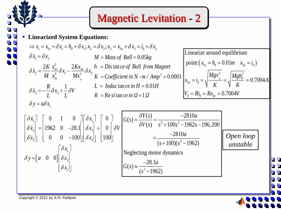
Magnetic Levitation - 2

Linearized System Equations:

1

1 1 1 0 1 2 2 3 3 3 0 3

1 2

2

3 32 1 33 2

1

3 3

1

; ;

22

1

e

e e

e e

e

x x x h x x x x x x i x

x x

x KxKx x x

M x Mx

Rx x V

L L

y a x

1

1 0 3 0

2 2

03 0

0 0 3

Linearize around equilibrium

point: 0.01

0.7004

0.7004

e

e e

e

e

x h m x i

Mgx Mghx i A

K K

V Ri Rx V

2

0 05

tan

0 0001

tan 0 01

Re tan 1

M Mass of Ball . kg

h Dis ce of Ball from Magnet

K Coefficient in N - m / Amp .

L Induc ce in H . H

R si ce in Ω Ω

1 1

2 2

3 3

1

2

3

0 1 0 0

1962 0 28.1 0

0 0 100 100

0 0

x x

x x V

x x

x

y a x

x

3 2

2

2

( ) 2810( )

( ) 100 1962 196,200

2810 =

( 100)( 1962)

Neglecting motor dynamics

28.1( )

( 1962)

Y s aG s

V s s s s

a

s s

aG s

s

Open loop

unstable


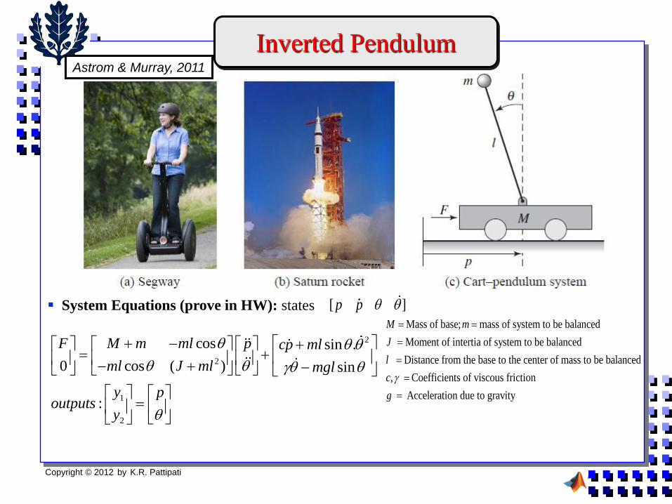
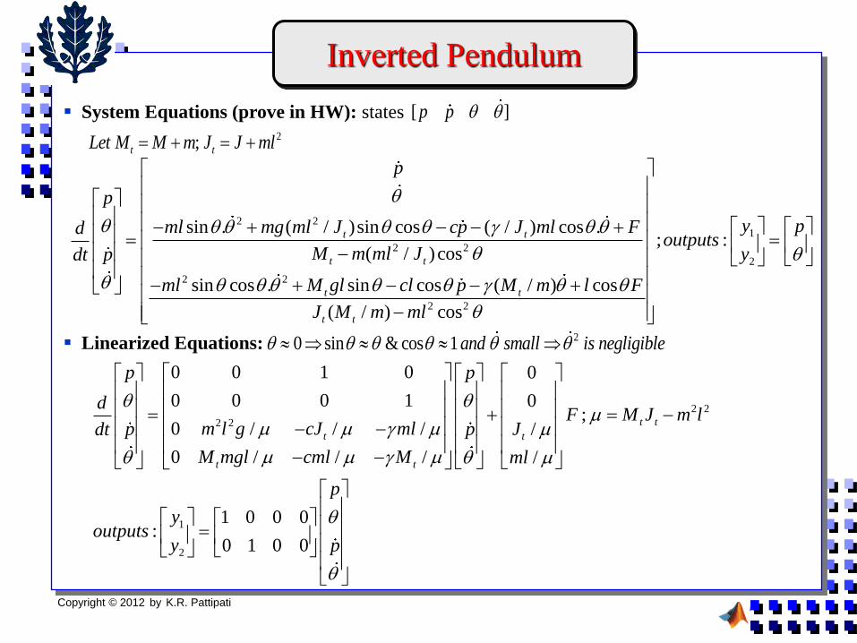
Inverted Pendulum

System Equations (prove in HW): states

2

2

1

2

cos sin .

0 cos ( ) sin

:

F M m ml p cp ml

ml J ml mgl

y poutputs

y

Mass of base; mass of system to be balanced

Moment of intertia of system to be balanced

Distance from the base to the center of mass to be balanced

, Coefficients of viscous friction

M m

J

l

c

g

Acceleration due to gravity

[ ]p p

Astrom & Murray, 2011


Inverted Pendulum

System Equations (prove in HW): states [ ]p p

2 21

2 2

2

2 2

2 2

sin . ( / )sin cos ( / ) cos .; :

( / ) cos

sin cos . sin cos ( / ) cos

( / ) cos

t t

t t

t t

t t

p

p

yml mg ml J cp J ml Fdoutputs

M m ml J ypdt

ml M gl cl p M m l F

J M m ml

p

2;t tLet M M m J J ml

2 2

2 2

1

2

0 0 1 0 0

0 0 0 1 0;

0 / / / /

0 / / / /

1 0 0 0:

0 1 0 0

t t

t t

t t

p p

dF M J m l

m l g cJ mlp p Jdt

M mgl cml M ml

p

youtputs

y p

Linearized Equations: 20 sin & cos 1and small is negligible


Spray Painting in an Automotive Plant -1

System Equations

• Inputs: Motor Torque, Tm is a function of line frequency, 0; Source voltage, v and

Motor speed, m (which is a state variable) There is inherent feedback already!

• Output: Pump speed, p

• Is the system linear? No, because Tm is a nonlinear function of {0, v and m}

• How to get state equations? Gears are not perfect; They have efficiency, < 1.

• How to get induction motor torque, Tm?

r : Gear Speed Ratio


Spray Painting in an Automotive Plant -1

System Equations

r : Gear Speed Ratio

r < 1 if p < m

Torque scales by 1/r

Electrical Analog

Electrical Analog

p

pb

mT

rTp

mmb

mJ

pT

pk

1

mr pJ

pmr

p

p

p

p

p

pppppp

ppmppmpp

m

m

p

m

m

m

mm

mpmmmm

ppm

TJJ

bbJT

krkrkT

TJ

TJ

r

J

b

TTr

bJ

TStates

1)3(

)()2(

1

)1(

,,:

Tm = Nonlinear f(0, v, m)

p= r m in steady state

supply radian frequency

supply voltage


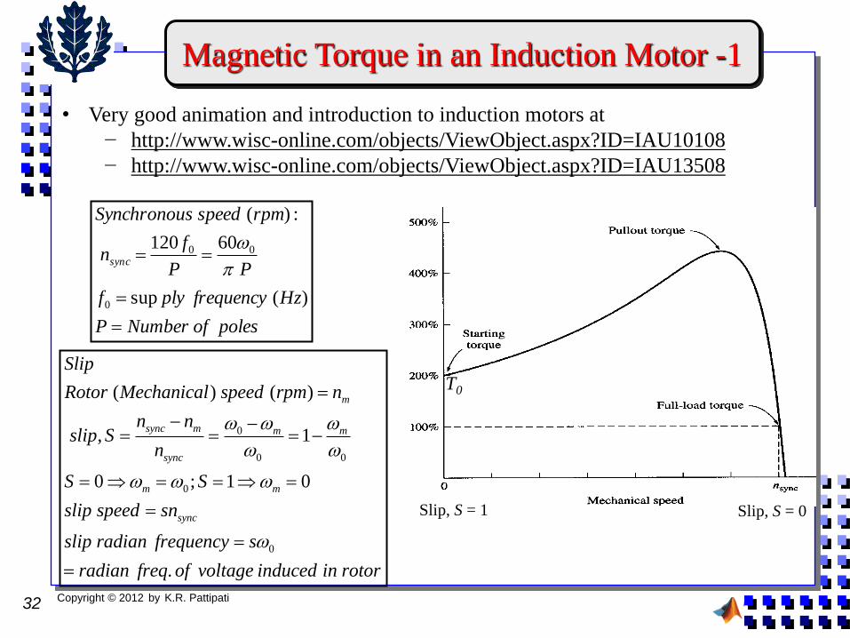
Magnetic Torque in an Induction Motor -1

polesofNumberP

Hzfrequencyplyf

PP

fn

rpmspeedsSynchronou

sync

)(sup

60120

:)(

0

00

• Very good animation and introduction to induction motors at



Slip, S = 0 Slip, S = 1

0

0 0

0

0

( ) ( )

, 1

0 ; 1 0

.

m

sync m m m

sync

m m

sync

Slip

Rotor Mechanical speed rpm n

n nslip S

n

S S

slip speed sn

slip radian frequency s

radian freq of voltage induced in rotor

T0








Magnetic Torque in an Induction Motor - 2

• Equivalent circuit of an induction motor. Assume 3 phases − Similar to a transformer except that the secondary windings rotate

− Frequency of voltage induced in the rotor is s0

− Voltage at s=0 is zero (no torque), Maximum at s=1

− ER0 = E1 NR / NS = E1 /aeff; ER = s ER0

stator

air gap

rotor

Equivalent circuit

Rotor Equivalent circuit

0

0

0

0

RR

R

RR

RR

jXs

R

E

jsXR

sEI

Rotor Equivalent circuit

2

2 0

2

2

2

1 0

eff R

eff R

R

eff

eff R

Seff

R

X a X

R a R

II

a

E a E

Na

N


Magnetic Torque in an Induction Motor - 3

• Final Equivalent circuit of an induction motor. Assume 3 phases

Actual rotor resistance

Resistance equivalent to

mechanical load

2

0

2

22

0

000

2

2

2

20

2

2

10

2

2

2

2

2

0

2

2

2

2

2

2

2

2

2

02

2

22

20

2

2

2

2

2

2

2

2

2

2

2

2

2

2

2

2

2)(3

13)1(3

,

)1(3,

mmm

m

mmSm

q

m

m

mmm

m

thatsuchSsmallforq

qTT

XR

RVTTwhere

SX

R

qST

SX

R

X

RS

TTXSR

SRVPT

XS

RS

SRVP

XS

R

VIimpedancestatorNeglecting

S

SRIPPowerMechanical

So, induction motors can be controlled by

varying 20, RorV


Steady-state Operating Point & Linearization

• Steady-state operating point

• State equations in matrix form

)(

)(;;

00

22

0

2

0

22

0

000

2

m

mmp

m

m

mm

p

mmmpppp

q

qbr

b

T

q

qT

brbTrbT

p

p

m

m

m

p

p

m

ppp

pp

mmm

p

p

m

Ty

T

J

T

JbJ

KrK

JrJb

T

100

0

0

/1

//10

0

0//

Nonlinearity enters only through Tm !


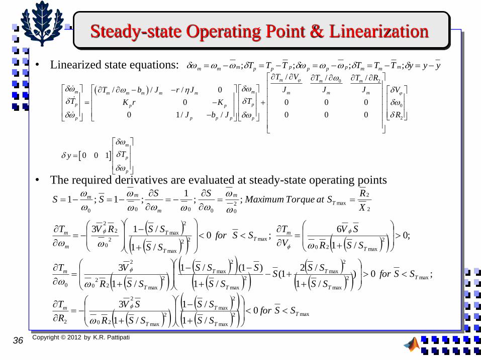
Steady-state Operating Point & Linearization

• Linearized state equations:

• The required derivatives are evaluated at steady-state operating points

yyyTTTTTT mmmppppppmmm ;;;;

0 2

0

2

/ / /

/ / / 0

0 0 0 0

0 1/ / 0 0 0

0 0 1

m m m

m m m m mm m m m m

p pp p

p p pp p

m

p

p

T V T T R

J J JT b J r J V

T TK r K

J b J R

Ty

max2

max

2

max

2

max20

2

2

max2

max

2

max

2

max

2

max

2

max22

0

2

0

2

max20

max22

max

2

max

20

2

2

2

2

max2

00000

0/1

/1

/1

3

;0)/1

/21(

/1

)1(/1

/1

3

;0/1

6;0

/1

/13

;;1

;1;1

T

T

T

T

m

T

T

T

T

T

T

m

T

mT

T

T

m

m

T

m

m

mm

SSforSS

SS

SSR

SV

R

T

SSforSS

SSS

SS

SSS

SSR

VT

SSR

SV

V

TSSfor

SS

SSRVT

X

RSatTorqueMaximum

SSSS


• We consider n state (x), m input (u), p output (y) systems (vectors are columns)

• The system dynamics are continuous, not discrete.

( , ); 0 initial stat

(1.1

e

, )(

x t f x t u t x

y t g x t u t

1 1 1

; ;

n m p

x t u t y t

x t u t y t

x t u t y t

(a) Linearized state space model

System matrix

Control matrix

Output matrix

I/O coupling matrix

A n n

B n m

C p n

D p m

• Multivariable LTI: linear and time-invariant Superposition and constant parameter

systems

;

(1.2)

[ ] [ ]; [ ] [ ]

; [ ] [ ]; [ ] [ ]

i iij ij

j j

i iij ij

j j

f fx t A x t B u t A a B b

x u

g gy t C x t D u t C c D d

x u

Math. Representation of (Sub)system Dynamics - 1



(b) Transfer function representation

1 1

1

0;

Laplace transform variable

( ) ( ) ( ) ( ) [ ( ) ] ( ) ( ) ( )

( ) ( ) ( ); 1,2,..,

( ) [ ( )] ( )

( )( ) |

(

(1.3)

) i

m

k kj j

j

kj

kkj u i

j

s

x s sI A B u s y s C sI A B D u s G s u s

y s g s u s k p

G s g s pby m transfer function matrix TFM

y sg s

u s

j

1

1; 1

1; 1

1; 1

m p SISO

m p SIMO

m p MISO

m p MIMO

(c) Impulse response representation

( )

0 0 0

( ) [Im Re ] [ ( )]

0; 0( )

( );

(

0

:

( ) ( ) ( ) ( ) ( 1.( 4) ) ( ) )

At

t t tA t

G s L pulse sponse L G t

tG t

Ce B D t t

Convolution Integral Formula

y t G t u d G u t d C e B u d D u t


(d) Variation 1: Disturbances, d and Measurement noise, v

(

( )

( ) ( ) = ( ) ( ) ( ) ( ) ( ) 1.5)

d

d d

x t Ax t Bu t B d t

y t Cx t Du t D d t v t y s G s u s G s d s v s

(e) Variation 2: Descriptor representation

1 (1 = ( ) ( ) [ ( ) ] ( ) .6)

Ex t Ax t Bu t

y t Cx t Du t

y s G s u s C sE A B D u s


39


Summary

1. What is Mechatronics?

2. Elements of Mechatronics

3. Mechatronics Applications

4. Example of Mechatronics Systems

5. Mathematical Modeling of Mechatronic Systems

6. General Representation of Systems

Lecture 1: Introduction & Mathematical Modeling

Documents