Lecture 1

Wave Phenomena Physics 15c

Lecture 1 Waves

Harmonic Oscillator

Administravia If you did not fill in the survey form last time, please do so   The forms are in the back of the hall

Online sectioning is on   Go to https://www.section.fas.harvard.edu/   Both discussion sections and lab sections   If the time slots do not work out for you, please send me email and

explain your constraints

Talk to me if you haven’t taken E&M (15b/153)

Today’s Goals Introduce the course topic: Waves   What do we study, and why is it worthwhile

Lots of recap today   Simple harmonic oscillators from 15a and 15b   Complex exponential, Taylor expansion   Make sure we all know the basics

Analyze simple harmonic oscillator using complex exp   How do we interpret the complex solutions for a physical system?   Are they general and complete?

Just how common are harmonic oscillators?   Very – Physics is filled with them   But why?

What we study in this course There are waves everywhere   Sea waves   Sound   Earthquakes   Light   Radio waves   Microwave   Human waves

The Great Waves off Kanagawa, Katsushika Hokusai, 1832

Features of waves Oscillation at each space point   Something (“medium”) is moving back and force

  Air, water, earth, electromagnetic field, people… Propagation of oscillation   Motion of one point causes the next point to move

  How does oscillation propagate over distance?   What determines the propagation speed?

We study the general properties of waves focusing on the common underlying physics

Waves and Modern Physics Modern (= 20th century) Physics has two pillars:   Relativity was inspired by the absoluteness of the speed of light =

electromagnetic waves   Quantum Mechanics was inspired by the wave-like and particle-like

behaviors of light

Everything is described by wave functions   Relativistic QM is a theory of generalized waves

Solid understanding of waves is essential for studying advanced physics

Goal of This Course Understand basic nature of wave phenomena   Intuitive picture of how waves work

  How things oscillate. How the oscillation propagates   How do waves transmit energy?   Why are waves so ubiquitous?

Foundation for more advanced subjects   Familiarity with wave equations   and Fourier transformation

Cover a few cool stuff related to waves   Esp. electromagnetic waves

Simple Harmonic Oscillators

C L

current

Already familiar with them, aren’t we?

Spring-Mass System Mass m is placed on a friction-free floor   Spring pulls/pushes m with force

(Hooke’s law)

  Newton’s law

We find the equation of motion:

  We must solve this differential equation for a given set of initial conditions

m

-x

x

F

F

F = ma = m

d 2xdt 2

F = −kx

m

d 2xdt 2 = −kx

Equation of Motion We know that the solution will look like a sine wave   Try   Equation of motion becomes

We’ve found a solution   Not necessarily the solution

Let’s remind ourselves how this solution looks like:   How the position and the velocity change with time   What is the frequency/period of the oscillation   How the energy is (or is not) conserved

x = x0 cosω t

md

dt 2 (x0 cosω t) = −kx0 cosω t

−mx0ω2 cosω t = −kx0 cosω t

ω =

km

Position, Velocity, Acceleration

  Oscillation repeats itself at ωt = 2π

  Position and velocity are off-phase by 90 degrees   Velocity is ahead

  Position and acceleration are off-phase by 180 degrees

x = x0 cosω t

v =dxdt

= −x0ω sinω t

a =dvdt

= −x0ω2 cosω t = −ω 2x

ω t

ω t

x0

−x0

x0ω

−x0ω

x = x(t)

v = v(t)

a = a(t)

ω t

−x0ω2

x0ω2

Frequency and Period ω in cosωt is the natural angular frequency of this oscillator   How much the phase of the cosine advances per unit time   Unit is [radians/sec]

The period T [sec/cycle] is given by

The frequency ν (Greek nu) [cycle/sec] is given by 2π =ωT → T =

2πω

= 2π mk

ν =

1T

=ω2π

=1

2πkm

a.k.a. Hertz

ω =

km

Energy Spring stores energy when stretched/compressed:

Moving mass has kinetic energy:

Therefore

ES =

12

kx2 =12

kx02 cos2 ω t

EK =12

mv 2 =12

mx02ω 2 sin2 ω t

=12

kx02 sin2 ω t Remember ω2 = k/m

ES + EK =

12

kx02 = constant.

Energy Tossing

Energy moves between the spring and the mass, keeping the total constant

ES =12

kx02 cos2 ω t

EK =12

kx02 sin2 ω t

12

kx02

12

kx02

12

kx02

ES

EK

ES

EK

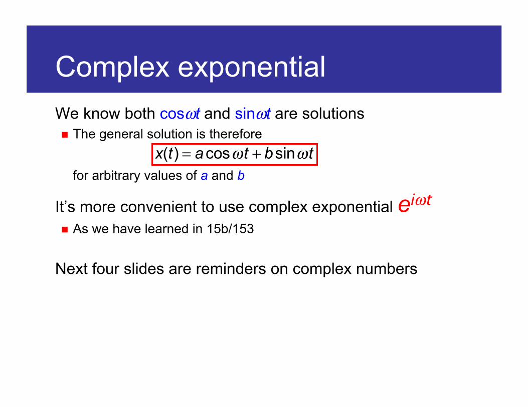
Complex exponential We know both cosωt and sinωt are solutions   The general solution is therefore

for arbitrary values of a and b

It’s more convenient to use complex exponential eiωt   As we have learned in 15b/153

Next four slides are reminders on complex numbers

x(t) = acosω t + bsinω t

Complex Numbers I assume you are familiar with complex numbers   A few reminders to make sure we got the key concepts

Complex plane

Real part

Imaginary part

Complex conjugate

Absolute Value and Argument For a complex number z,   The distance |z| from 0 is the absolute value:

  The angle θ is the argument, or phase:

z may be expressed as:

using Euler’s identity

θ = arg(z)

z = a2 + b2

z = z (cosθ + i sinθ) = z eiθ

eiθ = cosθ + i sinθ

Euler’s Identity

This is a “natural” extension of the real exponential   Check this with Taylor expansion

eiθ = cosθ + i sinθ

ex = 1+ x +

12

x2 +16

x3 +1

24x4 +

1120

x5 + ...

eix = 1+ ix −

12

x2 −i6

x3 +1

24x4 +

i120

x5 + ...

sin(x) = x −

16

x3 +1

120x5 − ...

cos(x) = 1− 1

2x2 +

124

x4 − ...

Complex Plane eiθ goes around the unit circle on the complex plane.

Re

Im

eiθ = cosθ + i sinθ

θ

http://xkcd.com/179/

Complex Solutions Revisit the simple harmonic oscillator:   Substitute

We got two complex solutions to a harmonic oscillator

  They are complex conjugates of each other   Generally, if you have a complex solution z(t) for an equation of

motion, the complex conjugate z*(t) must also be a solution

d 2xdt 2 = −ω 2x

d 2eXt

dt 2 = X 2eXt = −ω 2eXt

x = eXt

X = ±iω

x(t) = e± iω t

X2 = −ω 2

d 2z(t)dt 2 = −ω 2z(t)

d 2z*(t)dt 2 = −ω 2z*(t)

Complex Real Solutions Since the equation of motion is linear, any linear combination of z(t) and z*(t) is also a solution, i.e.,

Physical solution x(t) must be real

  Therefore

  Ignoring the factor 2, this is the real part of { arbitrary complex number α times one of the solutions z(t) }

x(t) = αz(t) + βz∗(t) where α,β are complex constants

Im(x(t)) = x(t) + x∗(t)2i

=αz(t) + βz∗(t)( ) − α∗z∗(t) + β∗z(t)( )

2i

=(α − β∗)z(t) − (α∗ − β)z∗(t)

2i= Im (α − β∗)z(t)( ) = 0

α = β∗ x(t) = αz(t) +α∗z∗(t) = 2Re(αz(t))

Complex Real Solutions Generally, when z(t) and z*(t) are complex solutions of an equation of motion, real (=physical) solutions are found by taking the real part of α⋅z(t), where α is an arbitrary complex constant

Going back to the harmonic oscillator:   Expressing α = a + ib, we get

  This is the general solution, as we knew from the beginning

We will use this recipe throughout the course

x(t) = Re (a − ib)eiω t( ) = Re (a − ib)(cosω t + i sinω t)( )= acosω t + bsinω t

Ubiquity of Harmonic Oscillators Harmonic oscillator’s equation of motion:

The restoring force –kx is linear with x   This is not exactly true in most cases   Springs do not follow Hooke’s law beyond elastic limits

Still, the physical world is full of almost-harmonic oscillators   And for a good reason

m

d 2xdt 2 = −kx Hooke’s Law force

Pendulum A pendulum swings because of the combined force of the gravity mg and the string tension T   Combined force is mg sinθ   Displacement from the equilibrium is Lθ   Force is not linear with displacement

A pendulum is not a harmonic oscillator Taylor-expand F = −mg sinθ around θ = 0

  For small angle θ,

θ

mg

T

mg sinθ

sinθ = sin0 + (sinθ ′)θ=0θ + 12 (sinθ ′′)θ=0θ

2 +

= θ − 16 θ

3 + 1120 θ

5 +

m

d 2 Lθ( )dt 2 = mLθ = −mgθ +O(θ3) Almost linear

Taylor Expansion Any (smooth) function f(x) can be approximated around a given point x = a as:

  You are already familiar with this The approximation is better when x − a is small   Because the higher-order terms (x – a)n shrinks faster

f (x) ≈ f (a) + ′f (a)(x − a) + 1

2′′f (a)(x − a)2 ++

1n!

f n(a)(x − a)n +

Look at the same problem with the potential energy   At angle θ, the mass m is higher than

the lowest position by h = L(1 – cosθ)   The potential energy is

EP = mgh = mgL(1 – cosθ)

Taylor-expand EP around θ = 0

  Differentiating the energy by displacement gives you the force

  OK, we got the linear force again…

Potential Energy

θ

L

h

x F = −

dEP

dx= −

1L

ddθ

12

mgLθ 2⎛⎝⎜

⎞⎠⎟= −mgθ

EP = mgL(1− cosθ) ≈ 12 mgLθ 2

cosθ = 1− 12θ

2 + 124 θ

4 −

Linearizing Equation of Motion We can often linearize the equation of motion for small oscillation around a stable point (equilibrium)

Why?   Anything that is stable is at a minimum

of the potential energy E   Let’s call it x = 0

  Taylor expansion of E near x = 0 is

  Since x = 0 is a local minimum, E′(0) = 0 and E′′(0) > 0   For small oscillations, higher-order terms (x3, x4, …) can be ignored

E(x) = E(0) + ′E (0)x +

12

′′E (0)x2 +16

′′′E (0)x3 + ... x

E

0

E(x) ≈ E(0) + 1

2′′E (0)x2 A simple parabola

Ubiquity of Harmonic Oscillators   This gives a linear force

Every physically stable object can make harmonic oscillation   Stable object sits where the potential energy

is minimum   The potential near the minimum looks like a

parabola   Its derivative gives a linear restoring force

This is true for small oscillation   How small depend on how the potential looks like   We observe oscillation only when “small” is large enough

x 0

F = −

dEdx

≈ − ′′E (0)x E(x) ≈ E(0) + 1

2′′E (0)x2

Summary Analyzed a simple harmonic oscillator   The equation of motion:   The general solution:

Studied the solution   Frequency, period, energy conservation

Learned to deal with complex exponentials   Makes it easy to solve linear differential equations

Studied how the equation of motion can be linearized for small oscillations   Taylor expansion of the potential near the minimum

Next: damped and driven oscillators

m

d 2x(t)dt 2 = −kx(t)

x(t) = acosω t + bsinω t ω =

km

where