Lec15 Impedance Matching and Tuning (I) 阻抗匹配和调谐hsic.sjtu.edu.cn/Assets/userfiles/sys_eb538c1c-65ff-4e82... · 2018-11-02 · 3 Impedance matching or tuning is important

Lec15 Impedance Matchingand Tuning (I)

阻抗匹配和调谐

2

The matching network（匹配网络） is ideally lossless（无耗）, to avoid

unnecessary loss of power, and is usually designed so that the impedance seen

looking into the matching network is Z0.

A lossless network matching an arbitrary load impedance to a transmission line.

Then reflections will be eliminated on the transmission line to the left of the

matching network, although there will usually be multiple reflections between the

matching network and the load. This procedure is sometimes referred to as tuning.

3

Impedance matching or tuning is important

Maximum power is delivered when the load is matched to the line (assuming

the generator is matched), and power loss in the feed line is minimized.

Impedance matching sensitive receiver components (antenna, low-noise

amplifier, etc.) may improve the signal-to-noise ratio (信噪比) of the system.

Impedance matching in a power distribution network (such as an antenna array

feed network) may reduce amplitude and phase errors.

4

Matching review

The power delivered to the load is

Load Matched to Line

Generator Matched to Loaded Line

Conjugate Matching

the maximum power delivered to the load.

5

As long as the load impedance, ZL, has a positive real part, a matching network can

always be found.

if

LLZ jX in 0 tanZ jZ l

6

Is a matching network unique for a particular system?

How to select a particular matching network?

• Complexity—As with most engineering solutions, the simplest design that satisfies

the required specifications is generally preferable.

• Bandwidth—Any type of matching network can ideally give a perfect match (zero

reflection) at a single frequency. In many applications, however, it is desirable to

match a load over a band of frequencies.

• Implementation—Depending on the type of transmission line or waveguide being

used, one type of matching network may be preferable to another. For example,

tuning stubs are much easier to implement in waveguide than are multisection

quarter-wave transformers.

• Adjustability—In some applications the matching network may require adjustment to match a variable load impedance.

7

5.1 MATCHING WITH LUMPED ELEMENTS (L NETWORKS)

The simplest type of matching network is the L-section, which uses two

reactive elements to match an arbitrary load impedance to a transmission line.

L-section matching networks. (a) Network for zL inside the 1 + j x

circle. (b) Network for zL outside the 1 + j x circle.

The reactive elements may be either inductors or capacitors, depending on the

load impedance.

8

If the frequency is low enough and/or the circuit size is small enough, actual

lumped-element capacitors and inductors can be used.

There are a large range of frequencies (usually >1GHz) and circuit sizes where

lumped elements may not be realizable. This is a limitation of the L-section

matching technique.

Two types of solutions:

•Analytic Solutions

• Smith Chart Solutions

9

Analytic Solutions

The circuit (a) should be used when zL = ZL/Z0

is inside the 1 + j x circle on the Smith chart,

which implies that RL > Z0 for this case.

The impedance seen looking into the matching network, followed by the load

impedance, must be equal to Z0

then

10

The solution is

Note that since RL > Z0, the argument of the second square root is always positive.

Then the series reactance can be found as

Two solutions are possible for B and X.

One solution, however, may result in significantly smaller values for the reactive

components, or may be the preferred solution if the bandwidth of the match is

better, or if the SWR on the line between the matching network and the load is

smaller.

11

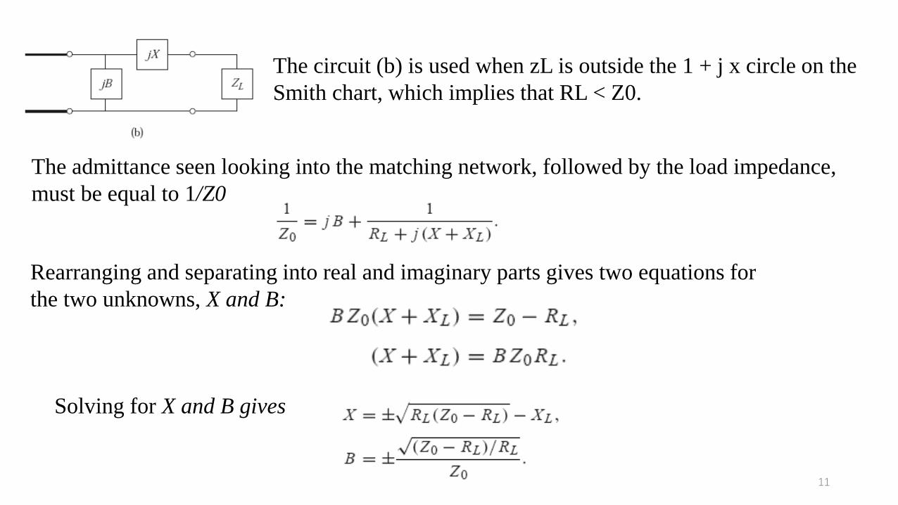
The circuit (b) is used when zL is outside the 1 + j x circle on the

Smith chart, which implies that RL < Z0.

The admittance seen looking into the matching network, followed by the load impedance,

must be equal to 1/Z0

Rearranging and separating into real and imaginary parts gives two equations for

the two unknowns, X and B:

Solving for X and B gives

12

Smith Chart Solutions

EXAMPLE 5.1 L-SECTION IMPEDANCE MATCHING

Design an L-section matching network to match a series RC load with an

impedance ZL = 200 − j100 to a 100 line at a frequency of 500 MHz.

Solution

1) The normalized load impedance is ZL = 2 − j1, which is plotted on the Smith chart.

This point is inside the 1 + j x circle, so we use the matching circuit of Figure a.

2) Because the first element from the load is a shunt susceptance (电纳),

it makes sense to convert to admittance by drawing the SWR circle through the load,

and a straight line from the load through the center of the chart,

0.4 0.2Ly j

13

ZL

yL

14

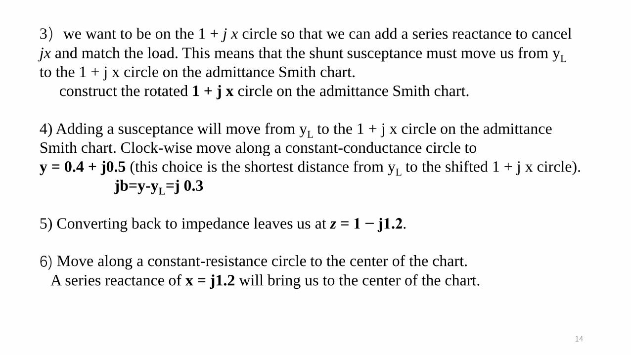
3）we want to be on the 1 + j x circle so that we can add a series reactance to cancel

jx and match the load. This means that the shunt susceptance must move us from yL

to the 1 + j x circle on the admittance Smith chart.

construct the rotated 1 + j x circle on the admittance Smith chart.

4) Adding a susceptance will move from yL to the 1 + j x circle on the admittance

Smith chart. Clock-wise move along a constant-conductance circle to

y = 0.4 + j0.5 (this choice is the shortest distance from yL to the shifted 1 + j x circle).

jb=y-yL=j 0.3

5) Converting back to impedance leaves us at z = 1 − j1.2.

6) Move along a constant-resistance circle to the center of the chart.

A series reactance of x = j1.2 will bring us to the center of the chart.

15

For comparison, the analytical formulas give the solution as b = 0.29, x = 1.22.

For a matching frequency of 500 MHz, the

capacitor has a value of

and the inductor has a value of

16

the second solution to this matching problem.

1) we will move to a point on the lower half of the shifted 1 + j x circle,

to y = 0.4 − j0.5. so b=y-yL=-0.7

2) Then converting to impedance z=1+1.2 and adding a series reactance ofx = −1.2 leads to a match as well.

Formulas (5.3a) and (5.3b) give this solution as

b = −0.69, x = −1.22.

17

the reflection coefficient magnitude

versus frequency for these two

matching networks, assuming that the

load impedance of ZL = 200 − j100

at 500 MHz consists of a 200 resistor

and a 3.18 pF capacitor in series.

There is not a substantial difference in bandwidth for these two solutions.

18

Lumped Elements for Microwave Integrated Circuits

such components can be used in hybrid and monolithic microwave integrated

circuits at frequencies up to 60 GHz, or higher, if the condition that < λ/10 is

satisfied.

19

5.2 SINGLE-STUB TUNING (单短截线调谐)

Another popular matching technique uses a single open-circuited or short-

circuited length of transmission line (a stub) connected either in parallel （并联） or in series （串联） with the transmission feed line （传输馈线） at a

certain distance from the load,

Such a single-stub tuning circuit is often very convenient because the stub can

be fabricated as part of the transmission line media of the circuit, and lumped

elements are avoided.

Shunt stubs （并联短截线） are preferred for microstrip line or stripline, while

series stubs （串联短截线）are preferred for slotline or coplanar waveguide.

20

Single-stub tuning circuits. (a) Shunt stub. (b) Series stub.

21

In single-stub tuning the two adjustable parameters are：the distance, d, from the load to the stub position,

the value of susceptance or reactance provided by the stub.

For the shunt-stub case, the basic idea is to select d so that the admittance, Y ,

seen looking into the line at distance d from the load is of the form Y=Y0 + j B.

Then the stub susceptance is chosen as −j B, resulting in a matched condition.

22

For the series-stub case, the distance d is selected so that the impedance, Z, seen

looking into the line at a distance d from the load is of the form Z=Z0 + j X. Then

the stub reactance is chosen as −j X, resulting in a matched condition.

The proper length of an open or shorted transmission line section can provide any

desired value of reactance or susceptance.

For a given susceptance or reactance, the difference in lengths of an open- or

short-circuited stub is λ/4.

23

Shunt Stubs

EXAMPLE 5.2 SINGLE-STUB SHUNT TUNING

For a load impedance ZL = 60 − j80 , design two single-stub (short circuit)

shunt tuning networks to match this load to a 50 line. Assuming that the load is

matched at 2 GHz and that the load consists of a resistor and capacitor in series,

plot the reflection coefficient magnitude from 1 to 3 GHz for each solution.

Solution(1) The first step is to plot the normalized load impedance zL = 1.2 − j1.6,

construct the appropriate SWR circle, and convert to the load admittance, yL

For the remaining steps we consider the Smith chart as an admittance chart.

(2) Notice that the SWR circle intersects the 1 + jb circle at two points, denoted as y1 and y2 in Figure 5.5a.

24

Thus the distance d from the

load to the stub is given by

either of these two intersections.

Reading the WTG scale, we

obtain

25

Actually, there is an infinite number of distances d around the SWR circle

that intersect the 1 + jb circle. Usually it is desired to keep the matching stub as

close as possible to the load to improve the bandwidth of the match and to

reduce losses caused by a possibly large standing wave ratio on the line between

the stub and the load.

At the two intersection points, the normalized admittances are

26

The length of a short-circuited stub that gives this susceptance can be found on the

Smith chart by starting at y =∞ (the short circuit) and moving along the outer

edge of the chart (g = 0) toward the generator to the −j1.47 point.

(3) Thus, the first tuning solution requires a stub with a susceptance of −j1.47.

The stub length is then

Similarly, the required short-circuit stub length for the second solution is

27

To analyze the frequency dependence of these two designs, we need to know

the load impedance as a function of frequency.

The series-RC load impedance is ZL = 60 − j80 at 2 GHz, so R = 60 and

C = 0.995 pF.

28

Observe that solution 1 has a significantly better bandwidth than solution 2; this is

because both d and stub length are shorter for solution 1, which reduces the

frequency variation of the match.

Reflection coefficient magnitudes versus frequency for the tuning circuits

29

Analytical solution

To derive formulas for d and, let the load impedance be written as

ZL = 1/YL = RL + j XL .

where t = tan βd. The admittance at this point is

where

30

Now d (which implies t) is chosen so that G = Y0 = 1/Z0.

Solving for t gives

The two principal solutions for d are

31

To find the required stub lengths, first use t in (5.8b) to find the stub susceptance,

Bs = −B. Then, for an open-circuited stub,

and for a short-circuited stub,

If the length is negative, λ/2 can be added to give a positive result.

for

for

32

Homework

33