LEARNING TO RECOGNIZE AGENT ACTIVITIES …arizona.openrepository.com/arizona/bitstream/10150/...LEARNING TO RECOGNIZE AGENT ACTIVITIES AND INTENTIONS by Wesley Nathan Kerr CC BY: C

Learning to Recognize Agent Activities and Intentions

Item Type text; Electronic Dissertation

Authors Kerr, Wesley

Publisher The University of Arizona.

Rights Copyright © is held by the author. Digital access to this materialis made possible by the University Libraries, University of Arizona.Further transmission, reproduction or presentation (such aspublic display or performance) of protected items is prohibitedexcept with permission of the author.

Download date 18/05/2018 02:02:42

Link to Item http://hdl.handle.net/10150/193649

LEARNING TO RECOGNIZE AGENT ACTIVITIES ANDINTENTIONS

by

Wesley Nathan Kerr

CC© BY:© C© Creative Commons 3.0 Attribution-Share Alike License

A Dissertation Submitted to the Faculty of the

DEPARTMENT OF COMPUTER SCIENCE

In Partial Fulfillment of the RequirementsFor the Degree of

DOCTOR OF PHILOSOPHY

In the Graduate College

THE UNIVERSITY OF ARIZONA

2010

2

THE UNIVERSITY OF ARIZONAGRADUATE COLLEGE

As members of the Dissertation Committee, we certify that we have read the dis-sertation prepared by Wesley Nathan Kerrentitled Learning to Recognize Agent Activities and Intentionsand recommend that it be accepted as fulfilling the dissertation requirement for theDegree of Doctor of Philosophy.

Date: 10 August 2010Paul R. Cohen

Date: 10 August 2010Niall Adams

Date: 10 August 2010Ian Fasel

Date: 10 August 2010Stephen Kobourov

Final approval and acceptance of this dissertation is contingent upon the candidate’ssubmission of the final copies of the dissertation to the Graduate College.I hereby certify that I have read this dissertation prepared under my direction andrecommend that it be accepted as fulfilling the dissertation requirement.

Date: 10 August 2010Dissertation Director: Paul R. Cohen

3

STATEMENT BY AUTHOR

This dissertation has been submitted in partial fulfillment of requirements for anadvanced degree at the University of Arizona and is deposited in the UniversityLibrary to be made available to borrowers under rules of the Library.

Brief quotations from this dissertation are allowable without special permission,provided that accurate acknowledgment of source is made. This work is licensedunder the Creative Commons Attribution-Share Alike 3.0 United States License. Toview a copy of this license, visit http://creativecommons.org/licenses/by-sa/3.0/us/or send a letter to Creative Commons, 171 Second Street, Suite 300, San Francisco,California, 94105, USA.

SIGNED: Wesley Nathan Kerr

4

ACKNOWLEDGEMENTS

I thoroughly enjoyed the time I spent in graduate school primarily because I workedwith exceptional people. There are many people that I would like to thank andacknowledge for their support over the past few years.

First among them is my advisor, Paul Cohen. I cannot begin to describe howincredible it was to work in Paul’s lab these past five years. I will simply say thatPaul is one of the most intelligent men I have ever met and it was a privilege tohave him as a mentor.

Special thanks goes to Niall Adams for the hard work he put in making thisdissertation what it is. He helped edit some of the earliest drafts and shaped someof the final experiments. Niall was a helpful mentor throughout my career andgenuinely concerned about making my research excellent.

Thanks goes to Stephen Kobourov and Ian Fasel for their contributions to mydissertation and for being part of my committee. I enjoyed our conversations andlook forward to future collaborations.

Growing up, my grandmother would remind me that “behind every great manthere is a great woman.” I do not claim to be a great man, but I can say that I havea great woman. My wife Nicole had the hardest job of all since she had to live withme while I was working on my dissertation. Her patience with me is admirable andher unwavering support is truly commendable.

There are several people I would like to thank from my time at USC. Firstamong them are my office mates, Shane Hoversten and Daniel Hewlett. I thoroughlyenjoyed our conversations, even though we did not always agree. I would also liketo thank you both for being friends and making me look back fondly at our timetogether at USC. Down the hall from my office were two other good friends whowould help bring a lighter side to my life as a graduate student. Many thanks toMartin Michalowski and Matt Michelson for always being up for a game of FIFAand a chance to relax.

I would like to thank the other graduate students from Paul’s lab: DanielHewlett, Derek Green, Antons Rebguns, Jeremy Wright, Nik Sharp, Anh Tran.I will cherish the conversations that we shared in the lab and at the bar.

Finally, a special thanks goes out to Lupe Jacobo and Rhonda Leiva for yourhard work ensuring that I would finish my dissertation in a reasonable time frame.

5

DEDICATION

Dedicated to Mom and Dad for their patience and support these last seven years.

6

TABLE OF CONTENTS

LIST OF FIGURES . . . . . . . . . . . . . . . . . . . . . . . . . . . . . . . . 8

LIST OF TABLES . . . . . . . . . . . . . . . . . . . . . . . . . . . . . . . . . 10

ABSTRACT . . . . . . . . . . . . . . . . . . . . . . . . . . . . . . . . . . . . 12

CHAPTER 1 INTRODUCTION . . . . . . . . . . . . . . . . . . . . . . . . 131.1 Motivation . . . . . . . . . . . . . . . . . . . . . . . . . . . . . . . . . 13

1.1.1 Intention . . . . . . . . . . . . . . . . . . . . . . . . . . . . . . 141.2 Problem . . . . . . . . . . . . . . . . . . . . . . . . . . . . . . . . . . 161.3 Overview . . . . . . . . . . . . . . . . . . . . . . . . . . . . . . . . . . 22

CHAPTER 2 RELATED WORK . . . . . . . . . . . . . . . . . . . . . . . . 232.1 Activity Recognition in Robots and Softbots . . . . . . . . . . . . . . 23

2.1.1 Intention . . . . . . . . . . . . . . . . . . . . . . . . . . . . . . 252.2 Computational Approaches . . . . . . . . . . . . . . . . . . . . . . . . 26

2.2.1 Pattern Mining . . . . . . . . . . . . . . . . . . . . . . . . . . 262.2.2 Multivariate Time Series Classification . . . . . . . . . . . . . 282.2.3 Univariate Time Series Classification . . . . . . . . . . . . . . 30

2.3 Remarks . . . . . . . . . . . . . . . . . . . . . . . . . . . . . . . . . . 31

CHAPTER 3 REPRESENTATION . . . . . . . . . . . . . . . . . . . . . . . 323.1 Qualitative Sequences . . . . . . . . . . . . . . . . . . . . . . . . . . . 33

3.1.1 Event Sequences . . . . . . . . . . . . . . . . . . . . . . . . . 343.1.2 Relational Sequences . . . . . . . . . . . . . . . . . . . . . . . 36

3.2 Real-Valued Variables . . . . . . . . . . . . . . . . . . . . . . . . . . 393.2.1 Preparation . . . . . . . . . . . . . . . . . . . . . . . . . . . . 393.2.2 Symbolic Conversion . . . . . . . . . . . . . . . . . . . . . . . 423.2.3 Shape Conversion . . . . . . . . . . . . . . . . . . . . . . . . . 43

3.3 Wrapping Up . . . . . . . . . . . . . . . . . . . . . . . . . . . . . . . 45

CHAPTER 4 LEARNING AND INFERENCE . . . . . . . . . . . . . . . . . 474.1 Sequence Similarity . . . . . . . . . . . . . . . . . . . . . . . . . . . . 47

4.1.1 Needleman-Wunsch Algorithm . . . . . . . . . . . . . . . . . . 494.1.2 Optimizations . . . . . . . . . . . . . . . . . . . . . . . . . . . 52

4.2 Signatures . . . . . . . . . . . . . . . . . . . . . . . . . . . . . . . . . 52

TABLE OF CONTENTS – Continued

7

4.3 Visualizing Signatures . . . . . . . . . . . . . . . . . . . . . . . . . . 554.4 Finite State Machines . . . . . . . . . . . . . . . . . . . . . . . . . . . 58

4.4.1 Signatures for Generalization . . . . . . . . . . . . . . . . . . 614.5 Inferring Hidden State . . . . . . . . . . . . . . . . . . . . . . . . . . 654.6 Wrapping Up . . . . . . . . . . . . . . . . . . . . . . . . . . . . . . . 67

CHAPTER 5 RESULTS . . . . . . . . . . . . . . . . . . . . . . . . . . . . . 695.1 Data Collection . . . . . . . . . . . . . . . . . . . . . . . . . . . . . . 69

5.1.1 Wubble World . . . . . . . . . . . . . . . . . . . . . . . . . . . 705.1.2 Wubble World 2D . . . . . . . . . . . . . . . . . . . . . . . . . 71

5.2 Classification . . . . . . . . . . . . . . . . . . . . . . . . . . . . . . . 745.2.1 Wubble World . . . . . . . . . . . . . . . . . . . . . . . . . . . 755.2.2 Wubble World 2D . . . . . . . . . . . . . . . . . . . . . . . . . 775.2.3 Discussion . . . . . . . . . . . . . . . . . . . . . . . . . . . . . 785.2.4 Learning Rate . . . . . . . . . . . . . . . . . . . . . . . . . . . 79

5.3 Heat Maps . . . . . . . . . . . . . . . . . . . . . . . . . . . . . . . . . 805.4 Recognition . . . . . . . . . . . . . . . . . . . . . . . . . . . . . . . . 835.5 Inferring Hidden State . . . . . . . . . . . . . . . . . . . . . . . . . . 855.6 Wrapping Up . . . . . . . . . . . . . . . . . . . . . . . . . . . . . . . 89

CHAPTER 6 APPLICATIONS TO DATA MINING . . . . . . . . . . . . . 916.1 Datasets . . . . . . . . . . . . . . . . . . . . . . . . . . . . . . . . . . 91

6.1.1 Handwriting . . . . . . . . . . . . . . . . . . . . . . . . . . . . 926.1.2 ECG . . . . . . . . . . . . . . . . . . . . . . . . . . . . . . . . 936.1.3 Wafer . . . . . . . . . . . . . . . . . . . . . . . . . . . . . . . 936.1.4 Japanese Vowel . . . . . . . . . . . . . . . . . . . . . . . . . . 936.1.5 Sign Language . . . . . . . . . . . . . . . . . . . . . . . . . . . 94

6.2 Classification . . . . . . . . . . . . . . . . . . . . . . . . . . . . . . . 956.2.1 k-NN Classifier . . . . . . . . . . . . . . . . . . . . . . . . . . 956.2.2 CAVE . . . . . . . . . . . . . . . . . . . . . . . . . . . . . . . 99

6.3 Wrapping Up . . . . . . . . . . . . . . . . . . . . . . . . . . . . . . . 102

CHAPTER 7 CONCLUSIONS AND FUTURE WORK . . . . . . . . . . . . 1047.1 Future Work . . . . . . . . . . . . . . . . . . . . . . . . . . . . . . . . 1057.2 Final Remarks . . . . . . . . . . . . . . . . . . . . . . . . . . . . . . . 107

REFERENCES . . . . . . . . . . . . . . . . . . . . . . . . . . . . . . . . . . . 109

8

LIST OF FIGURES

1.1 Heider and Simmel frame . . . . . . . . . . . . . . . . . . . . . . . . . 141.2 Sample PMTS for jump over . . . . . . . . . . . . . . . . . . . . . . . 181.3 Five examples of the activity approach . . . . . . . . . . . . . . . . . 19

2.1 Allen Relations . . . . . . . . . . . . . . . . . . . . . . . . . . . . . . 27

3.1 Diagram of common terms. . . . . . . . . . . . . . . . . . . . . . . . . 323.2 Example sequences for each representation . . . . . . . . . . . . . . . 353.3 The bit array for an approach episode . . . . . . . . . . . . . . . . . . 363.4 Compression process for CBA representation . . . . . . . . . . . . . . 373.5 The CBA representation for an approach episode . . . . . . . . . . . . 373.6 Speed time series . . . . . . . . . . . . . . . . . . . . . . . . . . . . . 403.7 The effects of smoothing. . . . . . . . . . . . . . . . . . . . . . . . . . 413.8 Speed time series with SAX symbols . . . . . . . . . . . . . . . . . . 443.9 Speed time series as SDL symbols . . . . . . . . . . . . . . . . . . . . 45

4.1 An alignment between two sequences. . . . . . . . . . . . . . . . . . . 484.2 Sample heat map with marked heat indexes . . . . . . . . . . . . . . 574.3 Heat maps for an approach episode . . . . . . . . . . . . . . . . . . . 594.4 An example of the activity approach marked as sequence of states. . . 594.5 An example of the conversion from a CBA into a FSM. . . . . . . . . 614.6 The complete FSM for each approach episode in Figure 1.3. . . . . . . 624.7 Mapping from mutiple sequence alignment to original episode . . . . 654.8 A general FSM for the approach activities in Figure 1.3 . . . . . . . . 66

5.1 Screenshot of the Wubble World 2D simulator. . . . . . . . . . . . . . 715.2 K-Folds partitioning . . . . . . . . . . . . . . . . . . . . . . . . . . . 765.3 Learning curve of the CAVE algorithm generated by presenting la-

beled training instances one at a time to corresponding signatures. . . 805.4 Heat maps for jump over and jump on aligned with a signature for

jump over . . . . . . . . . . . . . . . . . . . . . . . . . . . . . . . . . 815.5 The heat map for an approach episode aligned with the signature for

jump over. . . . . . . . . . . . . . . . . . . . . . . . . . . . . . . . . . 825.6 Recognition results . . . . . . . . . . . . . . . . . . . . . . . . . . . . 86

6.1 Classification accuracy for each representation after shuffling . . . . . 976.2 Difference in performance for ablation study . . . . . . . . . . . . . . 99

LIST OF FIGURES – Continued

9

6.3 Classification accuracy for each activity for different settings of theexclusion percentage. . . . . . . . . . . . . . . . . . . . . . . . . . . . 101

10

LIST OF TABLES

3.1 Fluent representation of an episode of approach. . . . . . . . . . . . . 343.2 SAX breakpoint lookup table . . . . . . . . . . . . . . . . . . . . . . 43

4.1 Similarity table for sequence alignment . . . . . . . . . . . . . . . . . 514.2 The signature constructed from the first four examples in Figure 1.3. 544.3 Signature update example . . . . . . . . . . . . . . . . . . . . . . . . 554.4 Sample signatures for each sequence representation . . . . . . . . . . 564.5 Rewriting the signature as a multiple sequence alignment. . . . . . . 64

5.1 Wubble World dataset statistics . . . . . . . . . . . . . . . . . . . . . 715.2 Wubble World 2D dataset statistics . . . . . . . . . . . . . . . . . . . 745.3 Classification results for Wubble World . . . . . . . . . . . . . . . . . 765.4 Wubble World confusion matrix . . . . . . . . . . . . . . . . . . . . . 775.5 Classification results for Wubble World 2D . . . . . . . . . . . . . . . 785.6 Classification results after shuffling sequences. . . . . . . . . . . . . . 795.7 Classification performance when some of the propositions are unob-

servable. . . . . . . . . . . . . . . . . . . . . . . . . . . . . . . . . . . 875.8 Inferred relations for the chase activity . . . . . . . . . . . . . . . . . 885.9 Overlap between α most frequent unobservable relations from the ww

dataset. . . . . . . . . . . . . . . . . . . . . . . . . . . . . . . . . . . 895.10 Overlap between α most frequent unobservable relations in ww2d sig-

natures . . . . . . . . . . . . . . . . . . . . . . . . . . . . . . . . . . . 89

6.1 Handwriting dataset statistics . . . . . . . . . . . . . . . . . . . . . . 926.2 Eclectrocardigram dataset statistics . . . . . . . . . . . . . . . . . . . 936.3 Wafer dataset statistics . . . . . . . . . . . . . . . . . . . . . . . . . . 936.4 Japanese vowel dataset statistics . . . . . . . . . . . . . . . . . . . . . 946.5 Auslan dataset statistics . . . . . . . . . . . . . . . . . . . . . . . . . 956.6 Percent correct with a 10-NN classifier from a 10-fold cross validation

classification task. . . . . . . . . . . . . . . . . . . . . . . . . . . . . . 966.7 A two-way analysis of variance for dataset by representation shows

one main effect and no significant interaction effect. . . . . . . . . . . 966.8 Best classification accuracy for several of our datasets. . . . . . . . . 966.9 Classification accuracy without SDL variables . . . . . . . . . . . . . 986.10 Classification accuracy without SAX variables . . . . . . . . . . . . . 996.11 A three-way analysis for the data shown in Figure 6.2. . . . . . . . . 100

LIST OF TABLES – Continued

11

6.12 The classification results for the CAVE classifier on six different rep-resentations. Results are reported from a 10-fold cross validationclassification task. . . . . . . . . . . . . . . . . . . . . . . . . . . . . . 100

6.13 A two-way analysis of variance for dataset by representation showstwo main effects and a significant interaction effect. . . . . . . . . . . 100

6.14 Pruning sensitivity results . . . . . . . . . . . . . . . . . . . . . . . . 102

12

ABSTRACT

Psychological research has demonstrated that subjects shown animations consisting

of nothing more than simple geometric shapes perceive the shapes as being alive,

having goals and intentions, and even engaging in social activities such as chasing

and evading one another. While the subjects could not directly perceive affective

state, motor commands, or the beliefs and intentions of the actors in the animations,

they still used intentional language to describe the moving shapes. The purpose of

this dissertation is to design, develop, and evaluate computational representations

and learning algorithms that learn to recognize the behaviors of agents as they per-

form and execute different activities. These activities take place within simulations,

both 2D and 3D. Our goal is to add as little hand-crafted knowledge to the rep-

resentation as possible and to produce algorithms that perform well over a variety

of different activity types. Any patterns found in similar activities should be dis-

covered by the learning algorithm and not by us, the designers. In addition, we

demonstrate that if an artificial agent learns about activities through participation,

where it has access to its own internal affective state, motor commands, etc., it can

then infer the unobservable affective state of other agents.

13

CHAPTER 1

INTRODUCTION

Humans are very adept at recognizing the activities that they participate in, as well

as the activities they observe other humans performing. For those of us who drive

into work, we must recognize when another driver is merging into the lane we cur-

rently occupy, otherwise we could end up in an accident. When we attend a football

game and have to sit in the top few rows of the stadium, we can still make out what

is going on, even though from that height the players on the field are nothing more

than blobs of color. It also seems as though we are not restricted to recognizing

the activities performed by other humans. For instance, Heider and Simmel (1944)

showed that human subjects observed a diverse set of activities when the scene con-

tained only a few geometric primitives (i.e. circles, squares, and triangles) moving

around on a white background (Figure 1.1). Subjects reported witnessing scenes

in which the geometric primitives were said to be fighting, chasing and fleeing, and

celebrating. Our ability to interpret the activities in such a limited scene makes

one believe that we could build a machine that could learn to recognize activities

as well. The purpose of this dissertation is to design, develop, and evaluate com-

putational representations and algorithms that are able to recognize the activities

agents perform.

1.1 Motivation

Humans are capable of recognizing many different activities and are not restricted to

human-human interaction or event animate-animate interaction. Often they involve

animate and inanimate entities, such as a child kicking a soccer ball, or something

as menial as eating dinner. Newtson (1973) demonstrated that subjects shown short

films of human behavior agreed with others on where the boundaries of an activity

14

occurred. Activities are perceived as discrete, with beginnings and ends, so although

people experience the world as a continuous flow of information, humans parse and

extract distinct activities. Furthermore, the activities and their boundaries are very

similar across different individuals.

Previous research has demonstrated that subjects who are shown animations

consisting of nothing more than simple geometric shapes perceive these shapes as

alive, having goals and intentions, and even interacting in social relationships such as

chasing and evading (Heider and Simmel, 1944; Blythe et al., 1999). For example,

subjects in the classic Heider and Simmel study were shown a two minute video

containing nothing more than a circle, two triangles (one large and one small), and

a few rectangles, yet the subjects consistently labeled the larger triangle as a bully

who constantly chased and harassed the smaller triangle and circle (Heider and

Simmel, 1944). A single frame from the original study is replicated in Figure 1.1.

Figure 1.1: Single frame from a similar animation to the original Heider and Simmelanimation.

1.1.1 Intention

Baldwin and Baird (2001) argued that we care little for the behavior exhibited by

animate entities in motion, and we are most interested in the underlying intentions of

the animate entities. Imagine that one is born with the ability to recognize patterns

in movement, but one is unable to discern any purpose behind these patterns. For

this individual, there is no difference between a playful shove from a friend or a shove

from someone wishing to cause harm to the individual. It is the shover’s intentions

15

that help determine the appropriate response. In general, humans appear to be very

good at inferring others’ intentions, so good, in fact, that we tend to infer intentions

often when there are none.

When human subjects ascribe intentions to geometric primitives like those shown

in Heider and Simmel’s research (see Figure 1.1), the question is which information

guides the process? Blythe et al. (1999) designed a task in which two adult sub-

jects each controlled his/her own artificial agent (a bug-shaped cursor) via a mouse.

Each subject was instructed to perform an activity, such as chase, flee, and fight.

The patterns of motion made by each participant were recorded and analyzed by

computational algorithms. There is no mechanism to record the intentions of the

bug-shaped cursor, but the subject acted with intent. Blythe et al. (1999) demon-

strated that just the actors’ patterns of motion in animations provide sufficient

information to classify their activities by the intentions of the subject controlling

the agent. In fact, the researchers’ classification algorithm outperformed human

subjects on the same task.

The heuristic algorithm Categorization by Elimination (CBE) developed by

Blythe et al. mapped patterns of motion onto class labels for intentional states;

however, this mapping does not improve its understanding of intentional states.

One of Heider and Simmel’s subjects described the larger triangle in Figure 1.1 as

“blinded by rage and frustration”; however, the CBE algorithm could not repli-

cate a similar description. Algorithms that classify activities by patterns of motion

understand physical activities but not their internal motivations (such as rage or

frustration), even if these words are provided as episode labels. So how might we

design algorithms capable of inferring intentional states?

In both the Heider and Simmel animations and the animations developed by

Blythe et al., subjects were only allowed to observe a subset of the features that

are available, i.e. positions, velocities, sizes, colors, etc. Both sets of animations

were designed to evoke the intentional state of entities within the animations, but

in neither case were the entities in the animations endowed with beliefs, desires,

and intentions. Subjects observing the animations could not directly perceive the

16

affective state, motor commands, or the beliefs and intentions of the actors or con-

trolling entities in the animations, yet they inferred affective states and described

them with intentional language.

We think humans infer affective states given non-affective observables such as po-

sitions and velocities by calling on their own affective experiences. Observables cue,

or cause to be retrieved from memory, representations of the activity that include

learned affective components, which are inferred or “filled in” as interpretations of

patterns of motion or other non-affective observables.

1.2 Problem

The problem addressed by this dissertation is to develop algorithms capable of

recognizing and classifying activities after only seeing a few episodes of the activity.

In addition, once the activity is correctly identified, there should be a mechanism

to infer the internal states of the agent performing the activity. For demonstrative

purposes, we focus on a single activity and highlight the different challenges that

we will face. We will be working with multivariate time series. A multivariate time

series (MTS) is a collection of random variables whose values are sampled over time

at the same intervals. Often, the values sampled in a MTS are real-valued, yet the

representations outlined in Chapter 3 operate on propositional data. We define a

propositional multivariate time series (PMTS) to be an MTS in which all of the

variables are propositions, and in Chapter 3 we outline a process to convert from

MTS into PMTS. A propositional variable can either be true or false at any moment

in time and can change value multiple times within a PMTS. A contiguous period of

time during which the propositional variable is true is called a fluent. Specifically, a

fluent is a tuple containing three elements: the name of the proposition, the time at

which it becomes true, and the time at which it becomes false. A collection of fluents

constitutes an episode, and instances of an activity are represented as episodes.

To illustrate, we use data from the Wubble World simulator. Wubble World

is a virtual environment with simulated physics, in which softbots, called wubbles,

17

interact with objects (Kerr et al., 2008). Wubble World is instrumented to collect

distances, velocities, locations, colors, sizes, and other sensory information and rep-

resent them with propositions such as Above(wubble,box) (the wubble is above

the box) and PVM(wubble) (the wubble is experiencing positive vertical motion).

Figure 1.2 shows an episode for the activity jump over. In this example, the grey

boxes are fluents and correspond to intervals during which the proposition is true.

As mentioned earlier, some of the variables are internal to the agent performing

the activity, e.g. the propositions Forward(agent) and Jump(agent) correspond

to unobservable motor commands that the agent performing the activity can exe-

cute. We separated the sample episode into phases in order to highlight some of the

structure present1. Any episode generated by an artificial agent jumping over a box

begins with an interval in which the box starts out in front of the agent, whereby

the agent moves more or less quickly towards the box. At some point, which will

vary between episodes, the agent will perform the jump action. Despite variations,

the activity jumping over a box contains a common pattern of intervals: the agent

moves towards the box (phase I), jumps upwards (phase II), moves above the box

(phase III), falls towards the ground (phase IV), and finishes on the ground behind

the box (phase V).

We assume that the episodes of an activity, such as jump over or jump on,

have some common structure. More colloquially, the fluents in similar episodes tell

the same story with minor variations. Thus, one may classify episodes by their

constituent patterns of fluents. This is not the only way to do it, however: a clean-

ing agent might classify cleaning episodes by the objects it interacts with, such as

pots and pans, rather than what was done with the pots and pans. However, our

focus here is classifying episodes by patterns of fluents. Figures 1.3(a)-(e) shows

four episodes of the activity approach. In each episode the triangle represents the

agent performing the approach, and the blue box represents the target of the ap-

proach. The PMTS for each approach is presented next to the corresponding visual

1We do not put any effort to discovering these phases in this dissertation, but in Chapter 7 we

discuss possible ways to discover phases.

18

I II III IV V

InternalMotor

Commands

Time

Phases

Figure 1.2: An example PMTS for the activity jump over. The activity is subdividedinto subregions for descriptive purposes.

schematic. Every example shares a common set of propositions, although not every

proposition becomes true in every episode. For instance, the visual schematic for

the approach in (a) does not contain a wall or a second box; therefore, these propo-

sitions never have the opportunity to become true. For the sake of brevity, we have

omitted additional variables that may also be necessary for classifying episodes of

approach, like internal desires and goals.

The purpose of this dissertation is to design, develop, and evaluate computa-

tional representations and learning algorithms that learn to recognize the activities

agents perform. The activities take place within simulation, either 2D or 3D. They

range from actions the agent is trying to perform, like jumping over blocks, to more

19

Visual Schematic PMTS

(a)

(b)

(c)

(d)

(e)

Figure 1.3: Five different visual and PMTS representations of the activity approach.Each example contains a red triangle approaching a blue square.

intentional actions such as chasing down another agent. In either case, some set

of variables will be provided as input to the algorithms that we develop. Some

variables are properties of the agents performing the activity; for example, we may

be interested in the location of an agent, the current heading of the agent, and the

velocity and speed with which the agent moves. Other variables that we may be

interested in concern the relations between multiple agents participating in the ac-

tivity. The list of relations includes the distance between the two agents, the relative

20

position of two agents, and the relative velocity of the two agents. Each observation

is real-valued, but we shall later see that we can convert these numbers into binary

propositions with a straightforward algorithm discussed in Chapters 3 and 6.

Our goals in this work are to add as little hand-crafted knowledge as possible to

the representation of episodes discussed in future chapters and to produce algorithms

that perform well over a variety of different activity types. Any patterns found in

episodes for similar activities should be discovered by the learning algorithm and

not by us, the designers. By different activity types, we mean activities outside the

domain of agent interactions, for example, another activity might involve recognizing

a subject’s handwriting or recognizing an abnormal heartbeat.

Performance is measured on three different tasks: classification, inference, and

recognition. In a classification task, the agent is presented with an episode it has

never encountered before and needs to produce the correct activity label to describe

the corresponding activity. The inference task requires the agent to infer the state of

internal variables over the course of the activity on the basis of previously observed

and labeled data. In inference, we are given the observable variables in the episode

and must correctly infer the internal state of the agents participating in the activity.

Inference can only be achieved if the agent can correctly classify episodes. The last

task is recognition, and it involves watching the state of the world change over time

and determining whether or not an activity has occurred. This task is intrinsically

harder than classification since the boundaries of an activity are not marked.

Some challenges are illustrated by the examples of approach activities introduced

in Figure 1.3. First, episodes have different durations. In each example in Figure 1.3

the agent is moving forwards towards the block and at some point, stops performing

the action forward(agent), while inertia continues moving the agent forward until

it comes to a stop in front of the box. Visually, this corresponds to a common

pattern, highlighted in red in Figure 1.3, that differs in duration for each episode.

A second challenge is to determine which of the many propositions are irrelevant

to the activity taking place. Sometimes examples of an activity contain additional

propositions, such as turn-left(agent) and turn-right(agent) in example (d).

21

These propositions are considered noise in the context of a specific activity; whereas,

the remaining propositions aid classification algorithms. Another example of irrel-

evant propositions is found in Figure 1.3(b). It just so happens that as the agent

is approaching the box, it also is approaching a wall behind the box. The variable

distance-decreasing(agent,box2) is not critical to a semantic interpretation of

approach and will only serve as a distraction in the classification task.

Even after determining which propositions to attend to, we still need to deter-

mine which fluents, if any, are important. It may be necessary to filter noisy fluents,

or it may just be the case that a certain fluent does not contribute anything to a se-

mantic interpretation of the activity. Consider the sample activity in Figure 1.3(e).

The agent must move around a wall that is blocking its path to the block it is ap-

proaching. Unlike the example in Figure 1.3(d), the agent moves parallel to the wall

and the distance to the block is not decreasing. Once the agent navigates around

the wall, then the distance begins decreasing again. In this example, there are two

fluents in which the proposition distance-decreasing(agent,box) becomes true.

None, one, or both of these fluents may help in the classification and prediction

tasks presented earlier.

In the coming chapters we will describe the CAVE algorithm, designed to classify

and visualize episodes. CAVE is trained to classify activities through supervised

learning with labeled episodes, such as instances of aggressive agents bullying smaller

agents. Visualization produces a descriptive image of the sometimes complex inter-

actions between fluents. An agent built with CAVE learns to classify activities by

first performing them itself. Therefore, it has access to both observable aspects of

activities such as motion, and private aspects such as intentions, emotional states,

and motor commands. It can also use observations of other agents to retrieve activ-

ities from memory and project the hidden or private aspects of these activities onto

other agents.

22

1.3 Overview

The rest of this dissertation is organized as follows. Chapter 2 provides a literature

review of previous relevant work done in artificial intelligence and data mining.

Chapter 3 details the representations designed to aid in the recognition of activities.

Chapter 4 details several learning and visualization algorithms the work directly

with the representation described in the preceding chapter. Chapter 5 provides

empirical results on several tasks within our agent base simulations. Chapter 6

provides a deeper analysis into the representations and algorithms within the agent

based simulations and across multiple datasets. Chapter 7 discusses avenues for

further research and draws some final conclusions.

23

CHAPTER 2

RELATED WORK

We divide this chapter into two sections. The first section highlights previous re-

search that addresses the same type of problem addressed by this dissertation,

specifically developing algorithms that learn to recognize the activities of agents

in simulators or robots in the real world, or reasoning about how humans learn

to recognize activities. The second section focuses on data-mining methods that

perform classification on univariate and multivariate time series without specifically

addressing activity recognition.

2.1 Activity Recognition in Robots and Softbots

There is a very similar line of research performed on robots that examine several

different methods by which a robot could learn to recognize activities. Firoiu and

Cohen (1999) describe a system composed of HMMs each trained on a batch of

robot episodes. The robot represents its experiences with the HMM and learns the

number of hidden states within the HMM via HMM state splitting. The focus of the

research seems to be more about how to redescribe the multivariate time series as a

set of logical variables rather than about learning a set activities in this environment.

In (Oates et al., 2000), the authors perform an experiment in which time se-

ries recordings are made of the sensors of a Pioneer-1 robot performing different

actions. The resulting time series are clustered using Dynamic Time Warping as

a distance metric between the time series. Although they do not explicitly model

entire activities, the authors show that the clusters found by agglomerative clus-

tering match those constructed by an expert. Similarly in (Rosenstein and Cohen,

1999) the authors propose to cluster the sensor recordings for a mobile robot. In

this instance, they first look for abrupt changes within sensor values as indication

24

that an event has occurred, and after finding events they cluster the time series to

generate signatures for the interaction.

More recently, Crick and Scasselatti developed a system for recognizing activi-

ties and simultaneously the intentions of the actors, all from a folk physics-based

interpretation of position and motion (Crick and Scassellati, 2008, 2010). This

work is an extension of previous work where the authors developed a system that

could correctly identify which player was “it” in a game of tag (Crick et al., 2007).

They found that when the robot was able to participate in playground games (like

tag), then it could recognize the intentions of other agents towards itself much more

quickly than if it was simply a passive observer. This was because it was able to test

its hypotheses about the other agents intentions towards it by approaching them.

The work primarily focuses on playground games such as tag and keep away. It

is unclear how the folk physics-based interpretation of intentions would extend to

activities with inanimate objects.

Pautler et al. (2009) propose a similar folk physics-based interpretation of in-

tention. In addition to recognizing intentions, the authors also focus on developing

agents capable of extracting explanations for these intentions. Explanations are gen-

erated when the agent’s assumptions about the environment are violated and other

agents are not acting in accordance to their perceived intentions. In both (Crick

and Scassellati, 2010) and (Pautler et al., 2009), the ability to recognize intentions

and the set of intentions that can be recognized are built into the agent, therefore no

learning that occurs. The method of inferring intention proposed in this dissertation

assumes that the agent learns about intentions of others by first experiencing those

intentions.

Breazeal et al. (2005) describe an implementation of facial imitation, which is

much more focused than general activity learning, but they have similar motivations

that guided the implementation. First, they argue that robots need to infer the

mental states of others in order to interact with them in a humanlike way, and they

believe that this will come from the observable behavior, as we noted in Chapter 1.

They also propose that one way infants learn is through imitative behavior. In our

25

terms, this would seem to be a way to generate more examples of an activity.

2.1.1 Intention

The notion of intention and recognizing the mental states of others is a becoming

a very popular topic for research. How does one infer the intentions of another?

We can take into account the age, sex, facial expressions, posture, communication

(in all forms), and the social context, but as Heider and Simmel have shown, we

do not need all of this information in order to make decisions about the intentions

of an animate agent. Sometimes, just movement information is enough. In Blythe

et al. (1999), human subjects controlled simulated insects on networked machines

to perform a variety of activities. Activities ranged from behaviors like chase and

flee to complex mating rituals that had one insect attempting to court another.

The authors trained a three-layer neural network to classify the activities based

on observable information, such as relative distance between the insects, relative

velocity, absolute velocity, relative heading, etc. The trained neural network and

heuristic based algorithm outperformed human subjects on a classification task.

Intention was not explicitly modeled in this system even though they system could

detect it through motion cues. In a followup study, Barrett et al. (2005) provide

results that suggest that our ability to infer the intentionality of agents (even simple

triangles) appears as young as 4 years of age, and we become more adept at it as we

age. Given a forced choice task with similar behaviors to the original study, subjects

correctly identified the right behavior in 80% of the samples.

Baker et al. (2009) demonstrate that goal inference can be accomplished by

Bayesian inverse planning. If we assume that planning models how an agent’s in-

tentions causes its behavior, then an observer can infer the agent’s intentions given

the observational behavior by inverting the planning process. Furthermore, the

learned Bayesian model accords well with human judgments of the intentions of a

simple goal seeking agent.

Recent research has proposed the mirror neuron system within humans as a

neural mechanism for recognizing and understanding the intentions of other peo-

26

ple (Iacoboni et al., 2005; Agnew et al., 2007). Although we do not claim that an

agent augmented with the representations and learning algorithms described in this

dissertation understands intentions in the same way that humans do, both lines of

research propose a mechanism by which one agent understands the intentionality

of another by relating the observed actions with one’s own previous memories and

internal states. We will see this trend again when we discuss the algorithm for

inferring intention in Chapter 4.

2.2 Computational Approaches

2.2.1 Pattern Mining

People have tried to solve many tasks that require as input multivariate time series.

Some of the earliest work set about trying to extract common patterns or rules

from propositional multivariate time series (PTMS). Most of this research focuses on

extracting temporal patterns that occur with frequency greater than some threshold,

also known as support. Temporal patterns are commonly described using Allen

relations (Allen, 1983). Allen recognized that there is only a small set of relationships

that two propositional intervals can be in, see Figure 2.1. The Allen relation between

two intervals is determined by the intervals’ start and end times.

In temporal pattern mining research, there are several critical choices that re-

searchers must make in order to find interesting patterns. First they must decide

on a measure that determines what makes one pattern better than another (often

called support). Secondly, researchers must select a representation of the temporal

relationships between propositions. Any representation must solve two problems:

First, a pattern consisting of 3 or more intervals can be represented as compositions

of Allen relations in several ways (e.g., we could say meets(a, (during(b, c))) or

during(meets(a, b), c)). A canonical form is desired, and is provided by several re-

searchers (Winarko and Roddick, 2007; Hoppner, 2001b). Second, a representation

should capture all the Allen relations that exist between propositions. A sentence

such as during(meets(a, b), c) does not say whether c occurs during a,b or both,

27

(x equals y)

(x meets y)

(x finishes-with y)

(x starts-with y)

(x overlaps y)

(x during y)

xy

xy

xyxy

xy

xy

(x before y)xy

(x e y)

(x m y)

(x f y)

(x s y)

(x o y)

(x d y)

(x b y)

Figure 2.1: Allen Relations

though one of these must be true.

Kam and Fu (2000) present an interesting canonical form, based on right con-

catenations, for compositions of three or more fluents. However, this representation

does not capture all the Allen relations in a composition. In the algorithm presented

by Kam and Fu, the frequency of the pattern was used to decide whether or not a

pattern was interesting. The algorithms presented in (Cohen, 2001; Cohen et al.,

2002; Fleischman et al., 2006) admitted a larger set of possible patterns than Kam

and Fu, but lacked a canonical representation of patterns. This research focuses on

extracting patterns that are determined to be statistically significant through hy-

pothesis testing. This is the only work we know of relating support for a pattern to

evidence against the null hypothesis that no pattern exists. Other research (Hoppner

and Klawonn, 2002; Winarko and Roddick, 2007) uses a matrix representation that

captures all k(k−1)2

pairwise Allen relations between k intervals, and again uses fre-

quency to determine the support of a pattern. In Hoppner and Klawonn (2002),

support is defined as the frequency within a sliding window, ensuring a degree of

locality between the internal relationships of the pattern, whereas in Winarko and

Roddick (2007) the support metric is similar to Kam and Fu (2000).

28

Papapetrou et al. (2009) propose a set of relations different from Allen relations

that afford more flexible matching between the input and relations. Essentially

Allen relations like the meets relation are relaxed to have fuzzy boundaries so that

one interval can end within ε of another interval beginning and it still be considered

meets. The mining algorithms rely on support, but the authors present different

methods to add constraints in order to speed up pattern generation and ignore

patterns that are not interesting.

Wu and Chen (2009) present an extension pattern mining problem so that

datasets can contain both point events and events with duration (intervals), called

a hybrid temporal pattern mining problem. Issues arise when one tries to extend the

pattern mining algorithms outlined earlier to handle point based events, and simi-

larly it is non trivial to extend algorithms capable of handling point based events,

but not interval events, e.g. Apriori (Agrawal and Srikant, 1994). The authors

extend the set of relations that occur between two events (point and interval) be-

cause Allen relations only considers interval events. The algorithm to mine patterns

extracts patterns with a support metric similar to those seen before.

Most of the representations and algorithms used are an extension of the Apri-

ori (Agrawal and Srikant, 1994) algorithm that performs a bottom up extraction

of patterns, and none of the work cited above focuses on classifying episodes. On

its own finding a large pattern in a set of episodes recorded from the same activity

does not tell one how to distinguish one activity from another, which is something

that we desire. We do not perform any pattern mining, via the methods outlined

above, in this dissertation, but previous work in this area influenced design decisions.

For instance, we treat all multivariate time series as propositional multivariate time

series. This allows us to describe patterns in the PMTS as a collection of Allen

relations.

2.2.2 Multivariate Time Series Classification

Batal et al. (2009) proposed a method for classifying multivariate propositional time

series. The authors first extract large patterns from the time series with methods

29

similar to those just discussed, but these patterns are based on a subset of the

original Allen relations, specifically before and overlaps. The complete set of large

patterns is pruned by hypothesis testing to generate a subset of patterns that will

serve as a binary feature vector. Each training episode results in a single binary

feature vector such that each value is true when the corresponding pattern is found

within the episode and false otherwise. The feature vectors and class labels are

used to train a traditional classifier (e.g. SVM). One problem with this approach is

that the classifier must be completely retrained whenever new training episodes are

acquired.

Kadous and Sammut (2005) present a multivariate classification algorithm that

operates on real valued time series and learns metafeatures to augment the original

data. Features cited as metafeatures include local maxima and gradient informa-

tion. These augment the original data with propositional features. A traditional

classifier is trained on all of the time series information, the original data and the

metafeatures. The rules generated from the classifier provide some insight into the

decisions made by the classifier.

Weng and Shen (2008) propose to use two-dimensional singular value decompo-

sition (2dSVD) as a tool for classifying multivariate time series. The authors treat

the MTS as a large two-dimensional matrix where each row is a different variable

and the columns correspond an observation at some specific moment in time. A fea-

ture matrix is obtained for each MTS and during classification a nearest-neighbor

classifier selects the class label for the most similar feature matrix. Other researchers

have preferred to classify time series by working directly on the original time series

without performing any transformations (Oates et al., 2000; Großmann et al., 2003;

Yang and Shahabi, 2007, 2004; Morse and Patel, 2007).

Another commonly used statistical approach to classification of multivariate time

series is to train hidden Markov models (HMM) (Nathan et al., 1995; Lee and Xu,

1996). HMMs have proven useful for speech recognition, as well as for classifying

words in American Sign Language (Starner, 1995). A commonly cited problem with

HMMs though is that the structure must be specified a priori. There have been

30

some approaches to help mitigate this problem; for instance, (Firoiu and Cohen,

1999) present a state splitting algorithm that attempts to learn the structure of the

HMM by greedily reducing the size of the resulting representation.

Gesture recognition in both 2D and 3D is a classification problem that involves

multivariate time series. In (Bobick and Wilson, 1995), the authors present algo-

rithms that reduce a multivariate time series into a single sequence of states and

then they employ a dynamic programming solution to find the distance between two

gestures.

2.2.3 Univariate Time Series Classification

There is far more research dealing with classification/clustering/indexing of univari-

ate time series than there is with multivariate time series. Within this research

there are several different problems being addressed. Some researchers focus on de-

veloping new distance metrics to compare univariate time series, while others focus

on reducing the amount of data used in comparisons. In addition, some researchers

examine ways to convert real-valued time series into symbolic sequences.

There are several different distance metrics for comparing two real-valued uni-

variate time series, and each of these has many extensions. One of the most straight-

forward is the longest common subsequence (LCS) algorithm. LCS provides a mech-

anism to align two time series that may suffer from translational shift (one starts

later than the other). It relies on dynamic programming to find the largest subse-

quence that is common between the two time series. One common way to do this

is to begin with real-valued time series, convert them into a symbolic form, then

use LCS as a distance metric to compare them (Devisscher et al., 2008; Balasko

et al., 2006; Wang et al., 2005). Some authors use LCS on the original, unaltered

time series by thresholding the equality operator when comparing two values in the

sequence (Vlachos et al., 2002, 2006; Buzan et al., 2004). Similarly, Chhieng and

Wong (2007) propose an extension to the string edit distance that relies on the dis-

tance between two points influencing the cost matrix setup by LCS and string edit

distance.

31

Another popular distance metric for comparing two univariate time series is

dynamic time warping (DTW). As the name implies, dynamic time warping was

designed to handle translational shifts in time and was originally created for speech

recognition (Sakoe and Chiba, 1978). One benefit of dynamic time warping is that

it can work directly on real-valued time series. Berndt and Clifford (1994) present

early results demonstrating the feasibility of DTW on univariate time series and

provide initial evidence that once DTW extracts patterns from the time series, then

we can construct higher order rules to describe transitions between the patterns.

Other researchers have used and extended DTW in order to perform classification

on univariate and multivariate time series (Oates et al., 1999; Keogh and Pazzani,

2001; Fu et al., 2008)

Most of the work on classification of time series data has focused on real valued

time series. In (Lin et al., 2003), the authors propose a new way to convert real-

valued time series into symbolic time series and demonstrate that even with a naive

distance calculation between symbolic time series, they are still able to generate

good results. Balasko et al. propose a way to convert a univariate time series into

a symbolic sequence and then perform sequence alignment in order to gather more

insight about the processes generating the time series (Balasko et al., 2006). The

authors do not perform a classification task and instead focus on understanding the

underlying process generating the time series.

2.3 Remarks

In this chapter, we could only scratch the surface on a large and diverse field. For

a thorough survey of temporal pattern mining and classification work see (Mitsa,

2010; Galushka et al., 2006; Liao, 2005).

32

CHAPTER 3

REPRESENTATION

In this chapter we outline the representations that will be used throughout the

dissertation. Recall that we are working with multivariate time series (MTS) in

which all of the variables are propositions, called PMTSs, and that PMTSs can be

decomposed into episodes that are collections of fluents (see Figure 3.1). Each fluent

is a tuple containing a proposition and the times at which the proposition becomes

true and false. A proposition can become true (and false) multiple times within an

episode, and each of these instances is represented as a separate fluent. Episodes

and their constituent fluents have different durations, start times, end times, and

propositions, so our representation of episodes must accommodate and generalize

over these variations (see Figure 1.3).

Episode

Activity: approach

proposition fluent

Figure 3.1: Common terms that will be used throughout the dissertation.

In Section 3.1, we define two classes of representation each focusing on differ-

ent aspects of the original PMTS representation. The representations differ in the

information that they retain. Many of the variables in the multivariate time series

33

explored in this dissertation are real-valued. To accommodate this type of variable,

we introduce a process to convert the range of real-valued variables into a set of

propositional variables in Section 3.2.

3.1 Qualitative Sequences

All of the representations that we outline here convert from a PMTS into a sequence

of tuples. The tuple is composed of a label (often referred to as the symbol) and

the fluents that participated in the label’s construction. Often in the presentation

of our sequences the fluents are ignored to present a concise view of the sequence.

Sequences have a rich history in the data mining literature with applications in

everything from biological sciences to natural language processing. Representing a

PMTS as a sequence of tuples whose labels can be compared as symbols allows us

to make use of prior research and we will demonstrate that these representations

perform well in a variety of data mining tasks. Thus the contributions of this

dissertation are not restricted to insights about recognizing activities, but include

methodology useful for multivariate time series data mining (see Chapter 6).

We propose two classes of representation, event and relational sequences. Multi-

ple sequence representations will be defined within each of these classes, each more

complex than the last, constructed from more or less of the information in the orig-

inal PMTS. In particular one might attend only to the start times or end times of

fluents, or to both start and end times. As we shall see in Chapters 5 and 6 different

representations lead to better performance at different tasks.

A single example, shown in the top half of Figure 3.2, illustrates different features

of all of the sequences that we propose. The example is one of our original episodes

of the activity approach and is reproduced from Figure 1.3(a). The PMTS as a

collection of fluents is shown in Table 3.1. As stated earlier a fluent is a tuple, so

the assertion (forward(agent) 0 11) means that proposition forward(agent) was

true in the discrete interval [0,11].

34

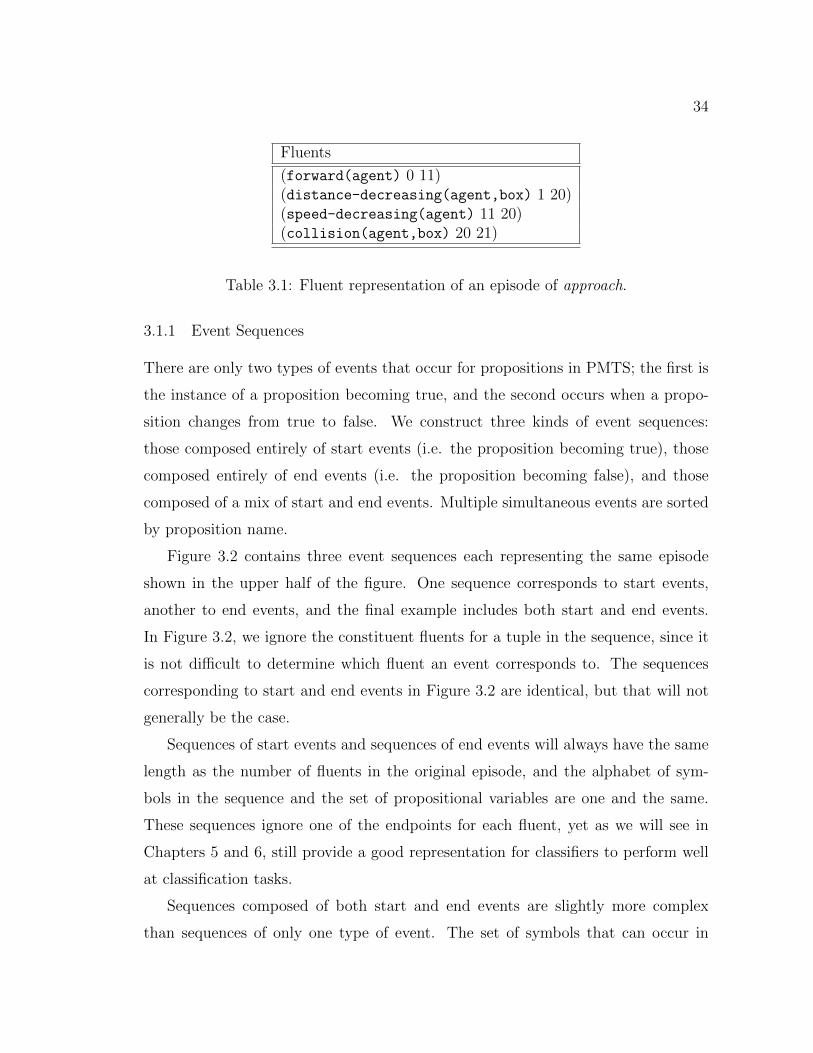
Fluents

(forward(agent) 0 11)(distance-decreasing(agent,box) 1 20)(speed-decreasing(agent) 11 20)(collision(agent,box) 20 21)

Table 3.1: Fluent representation of an episode of approach.

3.1.1 Event Sequences

There are only two types of events that occur for propositions in PMTS; the first is

the instance of a proposition becoming true, and the second occurs when a propo-

sition changes from true to false. We construct three kinds of event sequences:

those composed entirely of start events (i.e. the proposition becoming true), those

composed entirely of end events (i.e. the proposition becoming false), and those

composed of a mix of start and end events. Multiple simultaneous events are sorted

by proposition name.

Figure 3.2 contains three event sequences each representing the same episode

shown in the upper half of the figure. One sequence corresponds to start events,

another to end events, and the final example includes both start and end events.

In Figure 3.2, we ignore the constituent fluents for a tuple in the sequence, since it

is not difficult to determine which fluent an event corresponds to. The sequences

corresponding to start and end events in Figure 3.2 are identical, but that will not

generally be the case.

Sequences of start events and sequences of end events will always have the same

length as the number of fluents in the original episode, and the alphabet of sym-

bols in the sequence and the set of propositional variables are one and the same.

These sequences ignore one of the endpoints for each fluent, yet as we will see in

Chapters 5 and 6, still provide a good representation for classifiers to perform well

at classification tasks.

Sequences composed of both start and end events are slightly more complex

than sequences of only one type of event. The set of symbols that can occur in

35

the sequence is twice the size as the set of propositions, one symbol per proposition

for when it turns on (+) and one symbol per proposition for when it turns off (−).

Additionally, they will always be twice as long as the number of fluents in the episode

for the same reason. The resulting sequence for the episode in Table 3.1 is shown

in the lower half of Figure 3.2

Visual Schematic PMTS

Qualitative SequencesEvent Sequences Relational Sequences

start end both Allen CBA (Order 3)

f(a) f(a) f(a)+ (f(a) overlaps dd(a,b)) f(a) 110

dd(a,b) dd(a,b) dd(a,b)+ (f(a) meets sd(a)) dd(a,b) 011

sd(a) sd(a) f(a)− (dd(a,b) finishes-with sd(a)) sd(a) 001

c(a,b) c(a,b) sd(a)+ (f(a) before c(a,b)) f(a) 1100

dd(a,b)− (dd(a,b) meets c(a,b)) dd(a,b) 0110

sd(a)− (sd(a) meets c(a,b)) c(a,b) 0001

c(a,b)+ f(a) 100

c(a,b)− sd(a) 010

c(a,b) 001

dd(a,b) 110

sd(a) 010

c(a,b) 001

Keyc(a,b) collision(agent,box) f(a) forward(agent)

dd(a,b) distance-decreasing(agent,box) sd(a) speed-decreasing(agent)dd(a,b2) distance-decreasing(agent,box2) tl(a) turn-left(agent)di(a,b2) distance-increasing(agent,box2) tr(a) turn-right(agent)ds(a,b2) distance-stable(agent,box2)

Figure 3.2: The upper half of the figure is replicated from Figure 1.3(a) and showsan example of the approach activity. Underneath are all of the different sequencerepresentations for the example episode.

36

3.1.2 Relational Sequences

Relational sequences are composed of relationships between the fluents in an episode.

The most simple relationships contain two fluents, and can be described by the well-

known Allen relations (Allen, 1983). Allen recognized that, after eliminating sym-

metries, there are only seven relationships between two fluents, shown in Figure 2.1.

Allen relations capture all of the ordering relationships between the endpoints

of two fluents, but they do not easily extend to relationships between three or more

fluents. One way to describe all of the relationships between n fluents is to maintain

a n × n table of Allen relations, such that each row and column corresponds to a

single fluent from the PMTS and each cell stores the Allen relation between two

fluents (Winarko and Roddick, 2007; Hoppner, 2001a).

Alternatively, we could represent the original propositional data like the entries

in the upper half of Figure 3.2 as a bit array in which each row represents a logical

proposition, each column represents a moment in time, and each cell contains 1

or 0 depending on whether the corresponding proposition is true or false at that

moment. The corresponding bit array for the approach example in Figure 3.2 is

shown in Figure 3.3.

collision(agent, box) 00000000000000000001

distance− decreasing(agent, box) 01111111111111111110

forward(agent) 11111111111000000000

speed− decreasing(agent) 00000000000111111110

Figure 3.3: The bit array for the approach example in Figure 3.2

A related data structure, the compressed bit array (CBA), provides a canonical

representation of the complex patterns found in the PMTS. If we will be satisfied

with an ordinal time scale for patterns — a scale that preserves the order of changes

to a proposition’s status but not the durations of fluents — then we can compress

the bit array by removing identical consecutive columns, as shown in Figure 3.4.

The purpose of this compression is less to save space than to produce an abstraction

of the bit array in which patterns of changes that are identical but for their durations

37

are represented identically. The CBA corresponding to the dynamics in Figure 3.3

is shown in Figure 3.5.

1 1 1 1 1 1 1 1 0 0 0 0 0 0

0 0 0 0 1 1 1 1 1 1 1 1 1 1

1 1 0

0 1 1

Input Data CBA

p1p2

p1p2

Figure 3.4: Discarding all but one of identical columns (shown shaded) in a bit arrayproduces a compressed bit array (CBA).

collision(agent, box) 0001

distance− decreasing(agent, box) 0110

forward(agent) 1100

speed− decreasing(agent) 0010

Figure 3.5: The CBA representation for the approach example in Figure 3.2

It is important to note that the CBA representation conserves all of the Allen

relations present in the original PMTS. There is a direct mapping from the CBA

representation to the table representation outlined earlier, but we prefer the CBA

representation because it is easier to visualize the interactions between the proposi-

tions. The compressed bit array can be used to represent relationships between an

arbitrary number of fluents, known as the order of the CBA. CBAs generated from

pairs of fluents correspond directly with the Allen relations, and for simplicity, we

write these CBAs with the corresponding Allen relations.

In the previous discussion we described how to represent relations between flu-

ents, but not how to construct sequences from these relations. Now we present an

algorithm for generating an order k relational sequence from a PMTS composed

of the fluents F . Here we define k to be the number of fluents that participate in

each relationship varying from 2 . . . |F|. The first step is to enumerate all of the k-

combinations of fluents, of which there are(|F|

k

). A k-combination of fluents from F

is a set of k distinct fluents from F . Next the fluents in each k-combination are sorted

in order to generate a canonical representation of the CBA. Ordered fluents, also

38

known as normalized fluents, are sorted according to earliest start time (Winarko

and Roddick, 2007; Hoppner, 2001a). If two fluents start at the same time, they are

further sorted by earliest finish time, and if the start and end times are identical,

then they are sorted alphabetically by proposition name. A canonical representa-

tion of CBA ensures that we only work with one, not many, representations. Each

k-combination is a subset of the original set F , and can be written as a bit array.

Furthermore, this bit array can be compressed into a CBA via the process described

earlier. Finally, a tuple, containing the CBA as the label (or symbol) and the k

fluents that participate in the CBA, is appended to the sequence.

At this point, we have a sequence of tuples, one for each k-combination of fluents.

The tuples in this sequence lack any canonical order since until now they have just

been added to the sequence when they are discovered. As mentioned previously, we

hypothesize that activities have temporal order to them, and the resulting sequence

should try to preserve as much of that order as possible. Therefore, the tuples are

sorted by the earliest finishing CBA first, determined from the original fluents stored

as part of the tuple. Ties are broken by the earliest start time, then by individual

fluent start and end times, and if all other tie breakers fail we sort by proposition

names.

A qualitative sequence of CBA tuples can be shortened by defining a window

that determines how close any two fluents must be to consider one before the other.

This is known as the interaction window. There are two reasons why one might

define an interaction window. The first is that interactions between propositions

that are far apart in an activity are meaningless, and the second is that relational

sequences tend to be quite long and the interaction window is a heuristic to generate

smaller sequences. The interaction window is defined as follows. Assume that we

have two fluents (p1 s1 e1) and (p2 s2 e2) such that p1 and p2 are proposition names,

s1 and s2 are start times, e1 and e2 are end times, and e1 < e2. The two fluents

are said to interact if s2 ≤ e1 + w where w is the interaction window. If we set

w = 4 for the Allen sequence in Figure 3.2, then we would remove the relation

(forward(agent) before collision(agent,box)) ( (f(a) before c(a,b)) ) and

39

end up with a sequence with one less relation. The interaction window applies to

all of fluents within a CBA, and if any fluent is further than the interaction window

from all of the other fluents, then the CBA is disregarded.

Qualitative sequences reduce multivariate propositional time series to one di-

mensional sequences of relations between propositions. Sequences lose information

about the duration of the individual intervals, but retain information about the

start and end times of each interval relative to another, and preserve the temporal

order of CBAs. Assuming no pruning from an interaction window, the maximum

size of a sequence of order k CBAs generated from an episode containing n relations

is(nk

). Furthermore, if an episode has j propositions, then the alphabet size for the

symbols in the sequence is at least 7× (j2− j). it can be more if a proposition turns

on and off multiple times..

3.2 Real-Valued Variables

Variables within a time series often take on real values. Two such examples, common

to the types of activities we are interested in, are the distance between two moving

objects and the speed of an agent. In this dissertation, real-valued time series are

converted into collections of propositional time series. We will illustrate how this is

done with the time series called speed in Figure 3.6.

3.2.1 Preparation

We assume that there is error in the observations for our time series. This error could

come from faulty sensor readings on a robot or inaccurate physics approximations

in a simulated environment. If necessary, we first smooth the time series. Let X be

a univariate time series and let xi be one of the values of X. The smoothing process

works by modifying each value xi ∈ X, on the assumption that xi has an error

component that can be reduced by replacing xi by a weighted average of xi and its

neighbors. The effect of the moving averages smoothing technique is reduced error

so that sensors more closely approximate a smooth function. Although there are

40

Time

Speed

Figure 3.6: A time series showing the speed of an agent. The dashed line is thesmoothed version of the time series.

many ways to smooth univariate time series; Kalman filter (Kalman, 1960), kernel

smoothing (Hastie et al., 2001), etc., in this dissertation we employ a single, simple

technique. The moving averages smoothing algorithm is a type of mathematical

convolution governed by a single parameter k (Tukey, 1977). A new smoothed time

series is constructed by averaging all of the values within a sliding window of size

2k + 1.

More precisely, given a univariate time series X = x1, x2, . . . , xn and window size

k, we produce a smoothed time series Y = yk+1, . . . , . . . , yn−k such that each value

in Y is a weighted sum obtained by:

yt =1

2k + 1

k∑j=−k

yt+j t = k + 1, k + 2, . . . , n− k.

This technique is known as a “moving average” because each average is computed by

dropping the oldest value seen and including the next value. The average “moves”

through the time series computing yt until there are no new observations. Figure 3.6

demonstrates the effects smoothing the time series with a value of k = 25. The

jittery behavior of the speed variable is clearly removed. Selecting the “correct”

value of k hard. If k is too small then the jittery behavior remains, but if k is too

large then the shape of the curve could be altered. Figure 3.7 contains the original

41

time series speed and three different values of k, 5, 25, 100.

Time

Speed

Legend

k=25k=5

k=100

Original

Figure 3.7: The effects of the moving averages smoother on the original time seriesfor speed with three separate values of k.

The second step in the preparation of each univariate time series is standard-

ization. To standardize a time series, we first need to find the mean, x, and the

standard deviation, s, of the time series. We generate a new time series Z, such that

for each data point in the original time series we subtract the mean and divide by

the standard deviation:

zi =xi − xs

Each value in the resulting time-series is known as a z-score and it indicates how

many standard deviations above or below the mean the original observation was.

The resulting time-series will have a mean of zero and a standard deviation of one.

Standardizing time series does not change their shape. If two series do not look

like each other then standardizing them will not make them similar, and in this sense

standardizing cannot do any harm – but standardizing does remove differences due

to units of measurement. Standardizing two series makes them have the same mean,

and expresses each in standard deviation units. For instance, if X and Y are two

42

series and xi = myi for all xi and yi, then standardizing X and Y makes them

identical.

3.2.2 Symbolic Conversion

Lin et al. (2007) present an algorithm, called SAX, for converting a univariate real-

valued time series into a symbolic sequence. SAX produces a sequence of symbols,

S, given a series of z scores, Z, obtained by standardizing a series of reals, R. The

distribution of values in Z is assumed to be Gaussian, or Z ∼ N(0, 1). The claim

by the SAX authors that all time series have a Gaussian distribution is clearly

false, and it is unknown what effects this incorrect assumption has on performance.

Nevertheless, SAX provides a convenient method to convert real-valued time series

into symbols and overall performance is good, as seen in Chapters 5 and 6.

The SAX algorithm maps real values within intervals to symbols that identify

the intervals. The number of unique symbols generated by the SAX algorithm is

controlled by the parameter a. Selecting a determines how to select breakpoints

that divide the Gaussian distribution into a equally-sized areas. The assumption

of a Gaussian distribution allows us to determine the values of the breakpoints by

looking them up in a statistics textbook or in Table 3.2. We replace all of the

values in the standardized time series smaller than the smallest breakpoint with the

symbol a. Next we replace all of the values in the time series that are smaller than

the second smallest breakpoint with b, and so forth until all numbers are replaced

with symbols. The resulting SAX sequence is shown at the top of Figure 3.8 for

a = 3, and the bottom half presents the original time series with the breakpoints in

place.

The authors of the algorithm further show that the distance between two sym-

bolic sequences generated using SAX provides a lower bound on the distance between

the original two time series. This proof is an extension of the one that was generated

for the authors’ dimensionality reduction technique called PAA. We depart from the

original SAX algorithm at this point since we do not perform any dimensionality

reduction on our time series. Dimensionality reduction makes sense when all of the

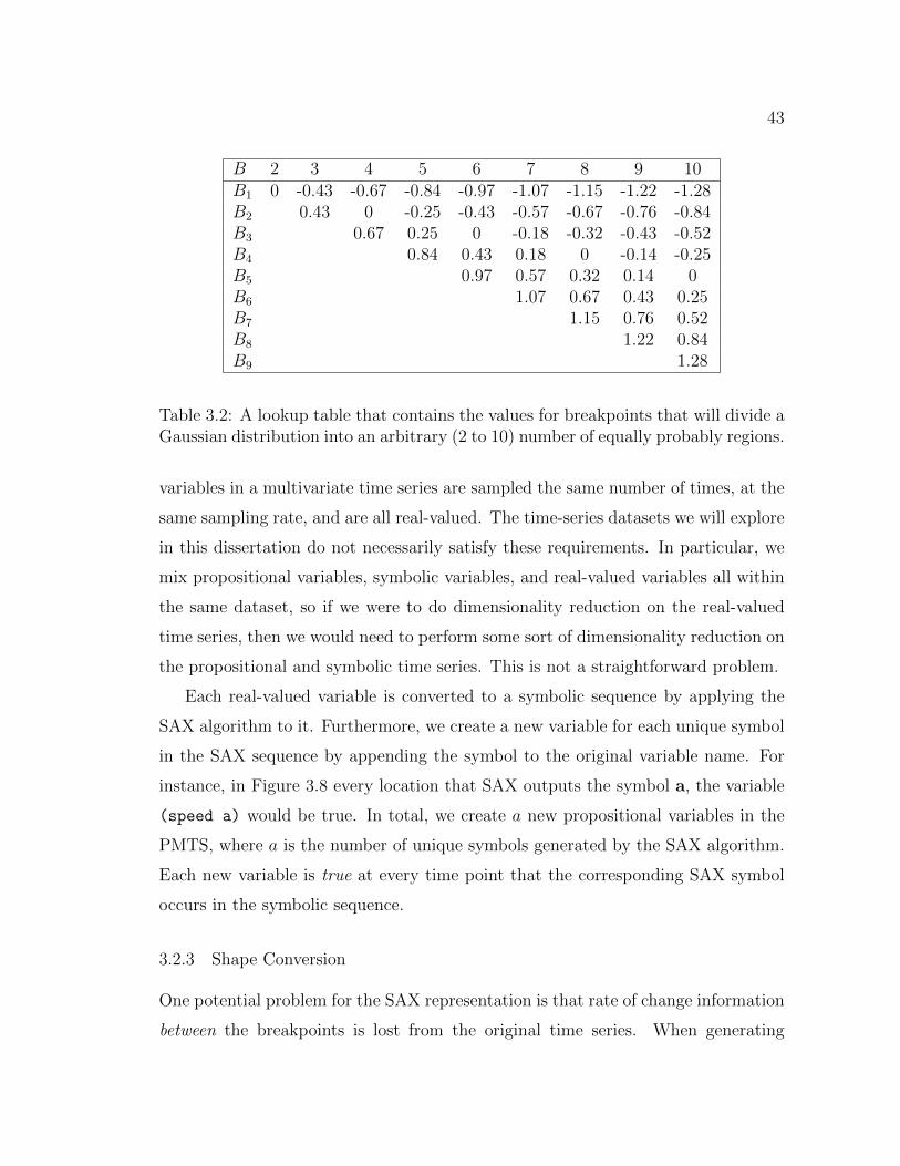
43

B 2 3 4 5 6 7 8 9 10B1 0 -0.43 -0.67 -0.84 -0.97 -1.07 -1.15 -1.22 -1.28B2 0.43 0 -0.25 -0.43 -0.57 -0.67 -0.76 -0.84B3 0.67 0.25 0 -0.18 -0.32 -0.43 -0.52B4 0.84 0.43 0.18 0 -0.14 -0.25B5 0.97 0.57 0.32 0.14 0B6 1.07 0.67 0.43 0.25B7 1.15 0.76 0.52B8 1.22 0.84B9 1.28

Table 3.2: A lookup table that contains the values for breakpoints that will divide aGaussian distribution into an arbitrary (2 to 10) number of equally probably regions.

variables in a multivariate time series are sampled the same number of times, at the

same sampling rate, and are all real-valued. The time-series datasets we will explore

in this dissertation do not necessarily satisfy these requirements. In particular, we

mix propositional variables, symbolic variables, and real-valued variables all within

the same dataset, so if we were to do dimensionality reduction on the real-valued

time series, then we would need to perform some sort of dimensionality reduction on

the propositional and symbolic time series. This is not a straightforward problem.

Each real-valued variable is converted to a symbolic sequence by applying the

SAX algorithm to it. Furthermore, we create a new variable for each unique symbol

in the SAX sequence by appending the symbol to the original variable name. For

instance, in Figure 3.8 every location that SAX outputs the symbol a, the variable

(speed a) would be true. In total, we create a new propositional variables in the

PMTS, where a is the number of unique symbols generated by the SAX algorithm.

Each new variable is true at every time point that the corresponding SAX symbol

occurs in the symbolic sequence.

3.2.3 Shape Conversion

One potential problem for the SAX representation is that rate of change information

between the breakpoints is lost from the original time series. When generating

44

3

-1

-0.5

0

0.5

1

1.5

2

2.5

Time

Speed

B3=0.67

B1=-0.67

dddddddddcccbbbbccccccccccccbbbbbbbbbbaaaaaaaaaaaaaaaaaaaaaaaaaaaaabbbbcccddd

B2=0.00

SAX

Figure 3.8: The time series for speed and corresponding SAX series of symbols.

symbols, the SAX algorithm relies entirely on which two breakpoints the recorded

value occurs between. Some derivative information is preserved by observing the

transitions between these symbols, but the question remains though as to whether

or not derivative information between the breakpoints is useful to the tasks outlined

in Chapter 1.

To explore the possibility performance can be improved by including the deriva-

tive information, we implemented a subset of the original shape definition library

(SDL) outlined in Agrawal et al. (1995), similar to Andre-Jonsson and Badal

(1997). We do not need the full expressivity of the original library and only en-

coded a subset of the primitive symbols. Converting from a real-valued time series

into symbols from our subset of SDL is accomplished in two steps. The first step is to

find the first difference of the time series which is the series of changes from one time

period to the next. For example consider the time series T = {1, 2, 4, 12, 10, 10, 8}.The first difference of T is the series T (1) = {1, 2, 8,−2, 0,−2}. Next we encode

each value in the first difference with a symbol from the set: up, down, stable. Up

corresponds to positive values in the first difference, down corresponds to negative

values, and stable means values that are approximately zero. In our example, the

symbolic sequence would be Ts = {up, up, up, down, stable, down}.As with the SAX algorithm, after running our SDL algorithm, we have a sequence

45

of symbolic values. So, we create three new propositional variables in the PMTS,

one for each variable and transition category label (up, down, stable). The new

variables are true at every time point that they occur in the symbolic sequence.

Figure 3.9 demonstrates the areas within the original speed time series that would

be encoded with the same symbol. The light gray regions represent periods of time

where the first derivative is stable, darker gray regions represent periods of time

where the first derivative is less than zero, and the darkest gray regions represent

periods of time where the first derivative is greater than zero.

3

-1

-0.5

0

0.5

1

1.5

2

2.5

Time

Speed

Figure 3.9: The time series for speed highlighted to show the symbols generatedthrough the conversion to our SDL.

The propositions constructed from the SDL conversion process aid performance

on the tasks outlined in Chapter 1. An analysis is included in Chapter 6.

3.3 Wrapping Up

In this chapter we outlined our qualitative sequence representation for propositional

multivariate time series. We provided additional algorithms for converting real-

valued univariate time series into multivariate propositional time series. We can

repeat this process for each real-valued variable within the original MTS. Depending

on the selected SAX alphabet size, a, each real-valued variable will result in a+3

new propositional variables in the final PMTS. Moving forward we explore how the

46

sequences will be used for recognizing activities.

47

CHAPTER 4

LEARNING AND INFERENCE

Recall the purpose of this dissertation: to design, develop, and evaluate computa-

tional algorithms that are able to recognize the behaviors of agents as they perform

and execute different activities. The previous chapter described the representations

of activities that we will be working with. In this chapter, we focus on the algorithms

that learn to recognize activities. The algorithms will be evaluated on two tasks:

classification and recognition. In the classification task, we are given an unlabeled

episode and must select the correct activity label, whereas in recognition we must

find episode boundaries and then determine which episode occurs if one occurs at

all.

To aid in both of these tasks, we describe and build an aggregate structure, called

a signature, from episodes of an activity. Episodes of an activity are represented as

sequences of tuples containing a symbol and the fluents that generated the symbol.

At its core the signature relies on sequence alignment to find similar subsequences

between it and another sequence. First we describe the process used to perform

sequence alignment. Next we discuss a novel algorithm that builds signatures from

episodes of an activity. Finally, we discuss several applications of signatures, such

as visualization and online activity recognition.

4.1 Sequence Similarity

In Chapter 3 we described two families of representations each composed of se-

quences of tuples. Each tuple is an ordered list containing a label (symbol) and the

set of fluents that participate in the label. In this section we ignore the fluents and

focus on the labels. We would like to identify similarities between sequences that

encode episodes from the same activity, for example we would like to identify the

48

similarities between the approach episodes described in Chapter 1. Furthermore, it

would be beneficial to use that measure of similarity to capture the distance from

one sequence to another. We would expect that episodes of the same activity have

small distances whereas two sequences from different activities would have larger

distances. A general solution to these tasks is to align the two sequences in such

a way as to maximize the overlap between them (de Carvalho Junior, 2002). We

choose to align the sequences because the tuples within the sequence are temporally

ordered and set intersection or simply counting the overlap would not take into

account this ordering.

We can easily visualize the alignment of two sequences by writing one sequence

on top of the other, as shown in Figure 4.1. The top sequence in Figure 4.1 is the

event sequence for the episode in Figure 1.3(c) and similarly the bottom sequence

is the event sequence for the episode in Figure 1.3(d). Spaces are inserted into the

top or bottom to break the sequences into smaller sequences so that the smaller

sequences have matching symbols. The resulting alignment ensures that the two

sequences are of equal length.

f(a) dd(a,b) dd(a,b2) − − − − sd(a) c(a,b)

l l l lf(a) dd(a,b) dd(a,b2) tr(a) tl(a) tr(a) di(a,b2) sd(a) −

Figure 4.1: An alignment between two sequences.

The objective of sequence alignment is to match as many symbols within the

sequences as possible. In the example, four symbols match; each highlighted with

a vertical bar. Spaces inserted into the alignment are represented as dashes. These

spaces produce gaps in the sequences, yet they are necessary to produce a good

alignment between the two sequences. Although not present in Figure 4.1 sym-

bols are sometimes substituted for each other. Visually, this would correspond to

one symbol being on top of another without a bar linking them. We can envision

instances where substitution would be useful, say when an agent approaches two dif-

ferent boxes in separate episodes of approach. In this case, the propositions would

almost completely match except for which box is being approached. Some of the

49

symbols in one episode could be substituted for others since the only differences

are minor. In general, this dissertation does not explore potential applications of

the substitution operator and effectively using the substitution operator is left for

future work (see Chapter 7).

One way to formalize the alignment between two sequences is to count the num-

ber of operations necessary to transform one sequence into the other. These oper-

ations include: insertion, deletion, and substitution. Assume we have two aligned

sequences X and Y; a gap in X corresponds to an insertion from Y into X, and a

gap in Y corresponds to a deletion from X. Substitution involves replacing a symbol

in one sequence with a symbol from the other sequence. The sequence of operations

to perform in order to convert one sequence into the other sequence is known as

the edit transcript. The sequence A can be converted into B in five steps: 1) insert

tr(a) after dd(a,b2); 2) insert an tl(a) after tr(a); 3) insert another tr(a) after

tl(a); 4) insert di(a,b2) after tl(a); 5) delete the final symbol c(a,b).

There are many possible alignments between two sequences, and each alignment

is scored according to the following procedure. Generally, we reward matches and

penalize mismatches. In the previous example, if we set the cost of performing an

operation (insertion, deletion) to -1, the cost of substitution to -1 and the reward

for matching to 2, then the alignment score would be 4× (2)+4× (−1)+1× (−1)+

0× (−1) = 3.

We define the similarity of two sequences to be the score for best alignment out

of all of the possible alignments between the two sequences. The similarity of two

sequences entirely depends on the amounts of rewards given for matches and the

costs assigned to the different operators for mismatches.

4.1.1 Needleman-Wunsch Algorithm

Needleman-Wunsch (Needleman and Wunsch, 1970) is the standard algorithm for

computing an optimal global alignment between two sequences. The algorithm

computes the similarity of two sequences X and Y with lengths m and n respectively.

The algorithm is based on dynamic programming, in that it builds up a complete

50

solution by examining and extending partial solutions. A partial solution involves

finding an optimal alignment between subsequences of the original sequences, i.e.

X[1 . . . i] and Y [1 . . . j].

The key recurrence in the sequence alignment problem is the observation that

the optimal alignment between the sequences X[1 . . .m] and Y [1 . . . n] is decided by

three values:

• the similarity of X[1 . . .m− 1] and Y [1 . . . n− 1] plus the cost of substituting

X[m] for Y [n]

• the similarity of X[1 . . .m− 1] and Y [1 . . . n] plus the cost of deleting X[m]

• the similarity of X[1 . . .m] and Y [1 . . . n− 1] plus the cost of inserting Y [n]

The cost of substituting X[m] for Y [n] is positive when the symbols match and

negative when they do not. The largest of three values in the recurrence is the

similarity score between X and Y . We can solve for the optimal similarity score

by constructing a (m + 1) × (n + 1) table S. Each cell in the similarity table

S[i, j] represents the similarity score between subsequences X[1 . . . i] and Y [1 . . . j].

Therefore S[i, j] denotes the minimum number of operations needed to transform

the first i symbols in X into the first j symbols in Y . Computing S[m,n] will give

the minimum number of operations to transform the sequences X and Y in their

entirety. We can compute S[m,n] by solving the more general problem S[i, j] for all

combinations of i and j. This is the standard dynamic programming solution and

there are three components to the solution.

First we must establish some base conditions, S[i, 0] = −i and S[0, j] = −j.These two base conditions capture the cost of inserting one complete sequence before

an empty sequence. The zero length sequence implied by both base conditions

restricts our choice of operations to insertion and deletion; either we insert the

symbols into the empty sequence or delete all of the symbols resulting in an empty

sequence.

51

Algorithm 1: SequenceAlignment

Input: sequences X,Y with lengths m,n

Output: (m+ 1)× (n+ 1) similarity table S

begin

for i=1 to m do

S[i][0]⇐ S[i− 1][0] + ins(X[i])

for i=1 to m do

S[i][0]⇐ S[i− 1][0] + del(Y[i])

for i=1 to m do

for j=1 to n do

diagonal ⇐ S[i− 1][j − 1] + sub(X[i], Y [j])

left ⇐ S[i][j − 1] + ins(X[i])

up ⇐ S[i− 1][j] + del(Y [j])

S[i][j]⇐ max(diagonal, left, up )end

Algorithm 1 provides the details for constructing the table S. The functions

sub(i, j), ins(i), and del(j) are the cost of substituting symbols X[i] and Y [j],

inserting symbol X[i], and deleting Y [j] respectively.

The table S is filled by row from left to right. The first row and first column

are filled in according to the base conditions, and the recurrence relation is used

to fill the table one row at a time. The cell S[m,n] contains the optimal similarity

score for the two sequences X and Y . Table 4.1 contains the similarity table for the

0 1 2 3 4 5∅ f(a) dd(a,b) dd(a,b2) sd(a) c(a,b)

0 ∅ 0 ← -1 ← -2 ← -3 ← -4 ← -51 f(a) ↑ -1 ↖ 2 ← 1 ← 0 ← -1 ← -22 dd(a,b) ↑ -2 ↑ 1 ↖ 4 ← 3 ← 2 ← 13 dd(a,b2) ↑ -3 ↑ 0 ↑ 3 ↖ 6 ← 5 ← 44 tr(a) ↑ -4 ↑ -1 ↑ 2 ↑ 5 ↑ 4 ↑ 35 tl(a) ↑ -5 ↑ -2 ↑ 1 ↑ 4 ↑ 3 ↑ 26 tr(a) ↑ -6 ↑ -3 ↑ 0 ↑ 3 ↑ 2 ↑ 17 di(a,b2) ↑ -7 ↑ -4 ↑ -1 ↑ 2 ↑ 1 ↑ 08 sd(a) ↑ -8 ↑ -5 ↑ -2 ↑ 1 ↖ 4 ← 3

Table 4.1: The similarity table S with arrows for tracing optimal alignments. Theoptimal alignment is highlighted by the light gray squares.

52

example shown in Figure 4.1.

Any similarity table also encodes the information necessary to determine the

optimal alignment. The optimal alignment is found by tracing a path in the table

from the last position back to the first position. The value in S[i, j] is determined

by the values in three surrounding cells (the recurrence relation). For example, if

S[i, j] = S[i − 1, j] + del(Y [j]), the trace reports a deletion of character Y [j] and

continues from cell S[i − 1, j], represented with arrows in Table 4.1. It is possible

to have more than one optimal alignment although our example only has one. All

optimal alignments can be found by tracing back all possible optimal paths through

the table S.

4.1.2 Optimizations

If we are only concerned with calculating the similarity score between two sequences,

then we do not need to store the entire table in memory. The similarity score is

stored in S[m,n] and the trace is not necessary to determine the score. As mentioned

previously, the score for any cell is determined by three other neighboring cells. As

the algorithm progresses by row, we need to store the previous row in order to access

two of the neighboring cells. The third neighbor is determined by the current row

and is always the last value that we calculated. This reduces the space cost from

n × m to 2n. This optimization is necessary in order to calculate some distances

between subsequences, because as we shall see in Chapters 5 and 6 we can generate

quite long sequences.

4.2 Signatures

The similarity score provides a mechanism to compare two sequences, but ultimately

we are interested in recognizing activities. We assume that we will have few to many

episodes of an activity, all represented as qualitative sequences. Signatures are an

aggregate structure constructed from examples of activities, designed to highlight

frequently occurring subsequences common to a majority of the examples.

53

Let S be a set of qualitative sequences with the same activity label. We define the

signature of the activity label, Sc, as an ordered sequence of weighted tuples. (The

only difference between a signature and a qualitative sequence is these weights.) In

the general case a single sequence can be considered a signature with each weight

set to 1. The signature learning algorithm, CAVE, is an incremental algorithm,

and works as follows: We select a sequence at random from S to serve as the

initial signature, Sc, and initialize all of its weights to 1. The signature, Sc, is

updated by combining it with the other sequences in S, processed one at a time. The

order that the sequences in S are processed is generally random. From a cognitive

science perspective, this just means that while learning about an activity, we cannot

guarantee the order that we will receive training episodes. In Chapter 7 we suggest

alternatives to processing sequences in a random order. A representative signature

constructed from the first four instances in Figure 1.3 is shown in Table 4.2.

Two problems are solved during the processing of the sequences in S. First,

the sequences are not identical, so Sc must be constructed to represent the most

frequent symbols in the sequences. The weights in Sc are used for this purpose.

Second, because a symbol can appear more than once in a sequence Si, there can

be more than one way to align Si with Sc. These problems are related because the

frequencies of symbols in Sc depend on how sequences are successively aligned with

it.

Updating the signature Sc with a sequence Si occurs in two phases. In the

first phase, Si is optimally aligned with Sc. The alignment algorithm, Needleman-

Wunsch, penalizes candidate alignments for symbols in Sc that are not matched by

symbols in Si, and rewards matches. Both the cost of insertion and the reward

for matching are determined by the weights stored with the signature as mentioned

above. Table 4.3 shows the signature from Table 4.2 aligned with the start event

sequence from the example in Figure 1.3(e). In the second phase, the weights in the

signature Sc are updated. If a relation in Si is aligned with one from Sc, then the

weight of this relation is incremented by one (e.g., the f(a) in Table 4.3). Otherwise

the weight of the relation is initialized to one (e.g., ds(a,b2) in Table 4.3) and it is

54

Symbols Weight

forward(agent) 4distance-decreasing(agent,box) 4distance-decreasing(agent,box2) 3distance-stable(agent,box2) 1turn-right(agent) 1turn-left(agent) 1turn-right(agent) 1distance-increasing(agent,box2) 1speed-decreasing(agent) 4distance-increasing(agent,box2) 1collision(agent,box) 3

Table 4.2: The signature constructed from the first four examples in Figure 1.3.

inserted into Sc at the location selected by the alignment algorithm.

Because the process of updating signatures does not remove anything from any

of the sequences in S, signatures become packed with large numbers of symbols

(propositions or Allen relations depending on the representation) that occur very

infrequently, and thus have low weights. Heuristics help reduce the number of low

frequency symbols occurring in each signature. We present one simple heuristic to

clean up the signature: After updating the signature t times, all of the relations

in the signature with weights less than or equal to n are removed. For example,

we set t = 10 and n = 3, meaning that the signature is pruned of all relations

occurring less than 4 times after a total of 10 training episodes. The signature is

again pruned after 20 training episodes, and so forth. The effects of pruning are

explored in Chapter 6.

In Table 4.4 we present signatures built from our examples of approach. In-

frequently occurring symbols, or symbols seen fewer than three times, have been

pruned from each of the signatures. The smallest signature is built from start event

sequences, and the longest signature is built from sequences composed of both start

and end events. In Figure 1.3 each example of approach has three red fluents cor-

responding to a shared pattern between the examples. This pattern is preserved in

55

Sc Aligned Si Aligned Sc Updated

f(a) f(a) f(a) 5dd(a,b) dd(a,b) dd(a,b) 5dd(a,b2) dd(a,b2) dd(a,b2) 4ds(a,b2) − ds(a,b2) 1tr(a) tr(a) tr(a) 2− ds(a,b2) ds(a,b2) 1

tl(a) tl(a) tl(a) 2tr(a) − tr(a) 1− dd(a,b) dd(a,b) 1

di(a,b2) di(a,b2) di(a,b2) 2sd(a) sd(a) sd(a) 5

di(a,b2) − di(a,b2) 1c(a,b) − c(a,b) 3

Keyc(a,b) collision(agent,box) f(a) forward(agent)

dd(a,b) distance-decreasing(agent,box) sd(a) speed-decreasing(agent)dd(a,b2) distance-decreasing(agent,box2) tl(a) turn-left(agent)di(a,b2) distance-increasing(agent,box2) tr(a) turn-right(agent)ds(a,b2) distance-stable(agent,box2)

Table 4.3: Updating the signature Sc. The leftmost column is the current signature(from Table 2). The second column is a sequence Si (from Table 1). The thirdcolumn is the optimal alignment of Si with Sc. The final column is the weights ofthe updated signature.

each of the signatures in Table 4.4. Each symbol with a weight of five corresponds

to some part of the original pattern, and only the signature constructed from CBAs

captures the entire pattern outlined in red with a single symbol (in Table 4.4 it is

the only CBA symbol with weight 5).

4.3 Visualizing Signatures

This section addresses two related challenges that remain after learning signatures

for activities using the methods developed in the previous section. The first is how

to visualize what CAVE has learned about activities, and the second is how to

visualize why a new episode should be labeled with a particular activity. Both of

these challenges are addressed by the visualization technique described next.

56

Event (starts) Event (ends) Event (both) Allen CBAf(a) 5 dd(a,b2) 3 f(a)+ 5 (f(a) c dd(a,b2)) 3 dd(a,b2) 0100

dd(a,b) 5 f(a) 5 dd(a,b)+ 5 (f(a) o dd(a,b)) 5 f(a) 1110 3dd(a,b2) 4 dd(a,b) 5 dd(a,b2)+ 4 (f(a) m sd(a)) 5 sd(a) 0001sd(a) 5 di(a,b2) 3 dd(a,b2)− 3 (dd(a,b) f sd(a)) 5 f(a) 110c(a,b) 3 sd(a) 5 f(a)− 5 (dd(a,b) m c(a,b)) 3 dd(a,b) 011 5

c(a,b) 3 sd(a)+ 5 (sd(a) m c(a,b)) 3 sd(a) 001c(a,b)+ 3 f(a) 1100dd(a,b)− 5 dd(a,b) 0110 3di(a,b2)− 3 c(a,b) 0001sd(a)− 5 f(a) 100c(a,b)− 3 sd(a) 010 3

c(a,b) 001dd(a,b) 110

sd(a) 010 3c(a,b) 001

Table 4.4: Signatures generated from training over the examples shown in Figure 1.3.Each signature is trained on the example episodes in order, and then we pruned allof the symbols seen fewer than three times.

Examples of an activity can be visualized by laying out constituent fluents on

a timeline; the signature of an activity, Sc, is not so easily visualized. Signatures

are made not of fluents but of tuples containing a symbol that could be a proposi-

tion name (event sequence), an Allen relation between fluents, or CBAs. Moreover,

signatures tend to be rather large until the low-weight symbols are pruned. Signa-

tures do not represent any single example of an activity, but rather are an aggregate

structure constructed from many examples of an activity. So signatures are too big

to visualize easily.

However, it is relatively straightforward to visualize the fit between a sequence

and a signature. Such a visualization shows whether the signature is a good fit to

the sequence, and which fluents in the sequence contribute most to the fit.

We developed a heat map representation of the alignment between a sequence,

Si, and a signature Sc. The heat map is a rendering of the original example as a

timeline with time flowing from left to right. Each proposition in the activity is

given its own row and the fluents for each particular proposition are rendered where

they occur in time. The color of the fluent conveys its importance; more important

fluents are darker and have a higher heat index.

In the discussions of representations and the learning algorithms, we ignored the

list of fluents attached to each symbol as part of the qualitative sequences. These

57

fluents become important now as we discuss how to determine the heat index of

an fluent. Let ρf = {τ1 . . . τN} be a set of tuples in the sequence Si that reference

the fluent f. When Si is aligned with a signature Sc, each tuple in ρf will either

match a symbol in Sc or it will not. The heat index for a fluent f is the sum of the

weights of the symbols in Sc that are matched by tuples in ρf . The heat indexes

for each interval in the original activity are normalized by the largest heat index

ensuring that heat index values range from zero to one. The heat index of an interval

determines its color in the heat map.

Signature Sequence(f(a) c dd(a,b2)) 3 (f(a) o dd(a,b))(f(a) o dd(a,b)) 5 (f(a) m sd(a))(f(a) m sd(a)) 5 (dd(a,b) f sd(a))

(dd(a,b) f sd(a)) 5 (f(a) b c(a,b))(dd(a,b) m c(a,b)) 3 (dd(a,b) m c(a,b))(sd(a) m c(a,b)) 3 (sd(a) m c(a,b))

Figure 4.2: A heat map generated from the approach signature trained on Allenrelations and the Allen sequence for episode (a) in Figure 1.3. The heat index foreach fluent is written on the fluent.

To illustrate why this is a good visualization technique, we present five heat maps,

one for each sequence representation (event and relational) on a single example of

approach. Each qualitative sequence is derived from the approach example shown in

Figure 1.3(e), and the signatures for each representation come from Table 4.4. We

chose this example because it highlights differences in the signatures that may not

have been apparent before, specifically how each signature handles the proposition

dd(a,b). This particular proposition is crucial to the activity of approaching a box.

In Figures 1.3(a)-(d), the proposition dd(a,b) only becomes true once, meaning

that once the agent starts towards the box, it does not falter. In Figure 1.3(e) it

becomes true twice, because the agent must navigate around a wall that is blocking

58

its path. This proposition is significant because it is common to every example of

approach, but in our example we have to distinguish between two fluents during

which the proposition is true.

Figure 4.3 contains each heat map. The heat map for the start event sequence

highlights the first fluent for proposition dd(a,b) because this type of sequence

focuses on start events and the first fluent happens to start when the rest of the

examples normally start, see Figures 1.3(a)-(d). The heat map for the end event

sequence shows that the alignment algorithm correctly identifies the second instance

of dd(a,b) which is expected since the proposition ends in the same order across

the examples in Figure 1.3. The heat map for the event sequence composed of both

start and end events highlights an interesting property of this type of sequence. We

have seen that the first instance of dd(a,b) is selected by the starts event sequence

(indicated by high intensity in the heat map) and the second instance of dd(a,b) is

selected by the ends event sequence (indicated by high intensity in the heat map).

Since start and end events are treated independently in the sequences of both starts

and end events, we see that the intensity is spread between both dd(a,b) fluents.

Some intensity was assigned to the first fluent because the start event matched, and

remaining intensity was given to the second fluent because the end event matched.

Our signatures are not perfect because some very intense fluents have no bearing

on the activity approach, and are considered noise fluents. Only the heat map for

the Allen relations representation correctly identifies the three fluents highlighted

in the original example, see Figure 1.3.

4.4 Finite State Machines

The qualitative sequence representations described in Chapter 3 are certainly not

the only way to represent propositional multivariate time series. Consider the first

example of approach replicated in Figure 4.4. The example is segmented into a

sequence of states such that each state is the current value of all of the propositions.

One could say that there are four states in Figure 4.4, in which different subsets of

59

Event (starts) Event(ends)

Event (both)

Allen CBA (order 3)

Figure 4.3: Heat maps generated by combining a sequence for Figure 1.3(e) withthe corresponding signature in Table 4.2.

the propositions are true (e.g., S1 = { forward(agent)}) and represent the sequence

as S1 → S2 → S3 → S4. A state in this sequence of states model is the same as a

column from the CBA representation discussed earlier.

S2 S3 S4S1

Figure 4.4: An example of the activity approach marked as sequence of states.

One way to use the sequences of states representation to recognize activities is to

construct a finite-state machine (FSM) to act as a recognizer. FSMs are a common

technique for modeling the behavior of a system and are represented by the tuple

(Σ,S, s0, δ,F) where: Σ is input alphabet , S is a finite number of states , s0 an initial

state, a δ is a non-deterministic state-transition function δ : S × Σ→ P(S), and F

60

is a set of final states. An example FSM is shown in Figure 4.5. The initial state

is filled in light gray, and nodes surrounded in double circles indicate final states.

Transitions are edges in the graph and are labeled with the input that induces the

transition. In general, inferring a FSM from positive an negative examples is a

known NP-complete problem (Gold, 1978), but we make no assertions about the

optimality of this FSM.

The conversion from a CBA into a FSM is straightforward, and Figure 4.5 con-

tains a CBA and the corresponding FSM. The input alphabet is a set containing

all possible columns in the CBA. Recall that the length of a column in the CBA

is equal to the number of propositions, therefore the size of the input alphabet is

exponential in the number of propositions. In the example, the alphabet size is

24 = 16 because we are only concerned with four of the propositions. The set of

states includes a state for each column in the CBA, as well as a start state. Each

state is identified by the column index as well as the column information. Since

there are exponentially many different inputs, we define a partial transition matrix.

The start state transitions to the state corresponding to the first column on input

that matches the first column. From there each state transitions to itself on input

that matches its corresponding column in the CBA, and each state transitions to

the state corresponding to next column on input that matches the next column.

Lastly, the final column in the CBA is added to the state of final states F . If we re-

ceive input in any state for which the transition is undefined, then we automatically

transition back to the start state.

With the example in Figure 4.5 we can recognize the approach activity as long as

it matches the example in Figure 4.4 exactly, but we know several more examples of

the approach activity, specifically those from (b) to (e) in Figure 1.3. We can build

a single FSM that accepts all of the examples by repeatedly converting from an

example into the CBA representation and finally into to same FSM with a different

branch from the start state. The resulting approach FSM can be seen in Figure 4.6.

To conserve space, the states and transitions are labeled with the propositions that

are true, and any other proposition not listed is assumed to be false. The result is

61

collision(agent,box) 0001

distance-decreasing(agent,box) 0110

forward(agent) 1100

speed-decreasing(agent) 0010

0110

0110

0101

0101

0101

1000

1000

0100

0110

0100

start

0100

Propositionsc(a,b)dd(a,b)f(a)sd(a,b)

Figure 4.5: An example of the conversion from a CBA into a FSM.

not a novel or all that interesting representation, but it is one that will recognize

a limited set of activities, specifically those that match a previously seen example.

What this representation lacks is any ability to generalize beyond the episodes it is

built from. Without additional knowledge, we do not know which propositions can

be safely ignored, and thus are left with an over-specialized FSM. In the next section

we discuss a mechanism to select propositions that are important and in addition

determine when those propositions are important, so as to reduce the state space.

Signatures constructed from qualitative sequences provide these mechanisms.

4.4.1 Signatures for Generalization

In this section we detail how a signature that maintains information about the

original episodes can be manipulated in order to construct a finite state machine

that generalizes better than the original.

Multiple Sequence Alignment

As discussed in previous sections, signatures are constructed from a set of qualitative

sequences. The signature maintains weights corresponding to the number of times

62

start

f(a)

f(a)

f(a)

f(a)

f(a) f(a)

f(a)

f(a)

f(a)

f(a)

f(a)

dd(a,b) f(a) dd(a,b)

f(a)

dd(a,b) f(a)

dd(a,b) sd(a)

dd(a,b)sd(a)

dd(a,b) sd(a)

c(a,b) c(a,b)

c(a,b)

f(a) dd(a,b)

dd(a,b2) f(a)

dd(a,b)dd(a,b2)

f(a)

dd(a,b) dd(a,b2)

f(a)

dd(a,b) ds(a,b2)

f(a)

dd(a,b)ds(a,b2)

f(a)

dd(a,b) ds(a,b2)

f(a)

dd(a,b) ds(a,b2)

sd(a)

dd(a,b)ds(a,b2)

sd(a)

dd(a,b) ds(a,b2)

sd(a)

dd(a,b) di(a,b2)

sd(a)

dd(a,b)di(a,b2)

sd(a)

dd(a,b) di(a,b2)

sd(a)

c(a,b) c(a,b)

c(a,b)

f(a)

dd(a,b) dd(a,b2)

f(a)

dd(a,b)dd(a,b2)

f(a)

dd(a,b) dd(a,b2)

f(a)

dd(a,b) dd(a,b2)

sd(a)

dd(a,b)dd(a,b2)

sd(a)

dd(a,b) dd(a,b2)

sd(a)

c(a,b) c(a,b)

c(a,b)

f(a)

dd(a,b) dd(a,b2)

f(a)

dd(a,b)dd(a,b2)

f(a)

dd(a,b) dd(a,b2)

f(a)

dd(a,b) dd(a,b2)

f(a) tr(a)

dd(a,b)dd(a,b2)

f(a)tr(a)

dd(a,b) dd(a,b2)

f(a) tr(a)

dd(a,b) f(a) tr(a)

dd(a,b)f(a)tr(a)

dd(a,b) f(a) tr(a)

dd(a,b) f(a) tl(a)

dd(a,b)f(a)tl(a)

dd(a,b) f(a) tl(a)

dd(a,b) f(a) tr(a)

dd(a,b)f(a)tr(a)

dd(a,b) f(a) tr(a)

dd(a,b) di(a,b2)

f(a) tr(a)

dd(a,b)di(a,b2)

f(a)tr(a)

dd(a,b) di(a,b2)

f(a) tr(a)

dd(a,b) di(a,b2)

sd(a)

dd(a,b)di(a,b2)

sd(a)

dd(a,b) di(a,b2)

sd(a)

f(a)

dd(a,b) dd(a,b2)

f(a)

dd(a,b)dd(a,b2)

f(a) dd(a,b) dd(a,b2)

f(a)

dd(a,b2) f(a) tr(a)

dd(a,b2)f(a)tr(a)

dd(a,b2) f(a) tr(a)

ds(a,b2) f(a) tr(a)

ds(a,b2)f(a)tr(a)

ds(a,b2) f(a) tr(a)

ds(a,b2) f(a)

ds(a,b2)f(a)

ds(a,b2) f(a)

ds(a,b2) f(a) tl(a)

ds(a,b2)f(a)tl(a)

ds(a,b2) f(a) tl(a)

dd(a,b) ds(a,b2)

f(a) tl(a)

dd(a,b)ds(a,b2)

f(a)tl(a)

dd(a,b) ds(a,b2)

f(a) tl(a)

dd(a,b) ds(a,b2)

f(a)

dd(a,b)ds(a,b2)

f(a)

dd(a,b) ds(a,b2)

f(a)

dd(a,b) di(a,b2)

sd(a)

dd(a,b)di(a,b2)

sd(a)

dd(a,b) di(a,b2)

sd(a)

Figure 4.6: The complete FSM for each approach episode in Figure 1.3.

that a symbol has been correctly aligned from the set of sequences. Another way

to view signatures is as a greedy heuristic that produces candidate solutions to the

multiple sequence alignment (MSA) problem. In the multiple sequence alignment

problem, we are presented with three or more sequences, and the task is to opti-

mally align all of the sequences with each other simultaneously. Finding an optimal

alignment for n sequences has been shown to be a NP-complete problem (Wang and

Jiang, 1994; Just, 2001), so for now we will be satisfied with signatures.

Signatures simply store the weight with each tuple in order to conserve space,

but we could maintain a solution to the current multiple sequence alignment of the

sequences encountered so far as a table. Each sequence would be given a row in the

table and each cell would contain the tuple corresponding the the type of sequence

(e.g. the name of a proposition for event sequences and the fluents that generated

the event). Table 4.5 contains the multiple sequence alignment for the five examples

from Figure 1.3. For demonstration purposes, we work with event sequences since

they have a smaller alphabet and smaller sequence size, but we are not restricted to

only event sequences. The sequences are aligned in order, so row one corresponds

to Figure 1.3(a), row two corresponds to Figure 1.3(b), and so forth. The totals at

63

the bottom of the table correspond to the weights that would be stored as part of

the signature (see Table 4.4).

Generalization

The signature and multiple sequence alignment table provide all of the information

necessary in order to determine which propositions and fluents can be ignored. First

we prune the multiple sequence alignment table by removing any columns from the

table that occur fewer than n times. For example, the table in the upper half of

Figure 4.7 contains the columns that occur three or more times in Table 4.5. All

others have been pruned away.

Each column that remains after pruning contains tuples from the original se-

quences, and each tuple consists of a symbol and the fluents that caused the sym-

bol’s generation. We can gather all of the fluents from a row in the MSA table (after

pruning) and reconstruct part of the original PMTS. It is assumed that through the

pruning process some of the fluents will be ignored. Figure 4.7 illustrates this idea.

Each cell in the table links to the original fluent that generated it. Green indicates

fluents that will are kept and the light blue fluents are ignored. In general, the set

of fluents kept will be the original set of fluents, but more often will contain a subset

of the original fluents. According to the signature, any fluents that are missing from

the reconstruction of the PMTS can be ignored.

The next step is to generate a FSM like in Figure 4.6, but the CBAs that will

be converted into the new FSM will be generated from pruned sets of fluents. An

example of the generalized FSM is shown in Figure 4.8. Since we only keep a subset

of the original fluents, each of the branches in Figure 4.8 tends to be shorter than

its corresponding branch in Figure 4.6.

We also introduce a slight relaxation to the FSM representation outlined earlier.

In all of the previous examples, the state and input specified which of the proposi-

tions must be true and which must be false. The relaxation that we propose is that

any proposition not listed as part of the state is ignored, i.e. the proposition can

be either true or false. The relaxed FSM (shown in Figure 4.8) will accept a more

64

f(a)

dd

(a,b

)sd

(a)

c(a,b

)

f(a)

dd

(a,b

)d

d(a

,b2)

ds(

a,b

2)

sd(a

)d

i(a,b

2)

c(a,b

)

f(a)

dd

(a,b

)d

d(a

,b2)

sd(a

)c(

a,b

)

f(a)

dd

(a,b

)d

d(a

,b2)

tr(a

)tl

(a)

tr(a

)d

i(a,b

2)

sd(a

)

f(a)

dd

(a,b

)d

d(a

,b2)

tr(a

)d

s(a,b

2)

tl(a

)d

d(a

,b)

di(

a,b

2)

sd(a

)

Tot

als

55

41

21

21

12

51

3

Tab

le4.

5:R

ewri

ting

the

sign

ature

asa

mult

iple

sequen

ceal

ignm

ent.

65

(f(a) [·]) (dd(a,b) [·]) (sd(a) [·]) (c(a,b) [·])(f(a) [·]) (dd(a,b) [·]) (dd(a,b2) [·]) (sd(a) [·]) (c(a,b) [·])(f(a) [·]) (dd(a,b) [·]) (dd(a,b2) [·]) (sd(a) [·]) (c(a,b) [·])(f(a) [·]) (dd(a,b) [·]) (dd(a,b2) [·]) (sd(a) [·])(f(a) [·]) (dd(a,b) [·]) (dd(a,b2) [·]) (sd(a) [·])

Totals 5 5 4 5 3

Figure 4.7: A demonstration of how a row in the pruned multiple sequence alignmenttable is mapped back to the original episode.

diverse set of episodes than the original FSM (shown in Figure 4.6), although not

every accepted episode will necessarily be an example of the activity the FSM was

designed to accept. In the next chapter we evaluate the performance of both FSMs

on a recognition task.

The general FSM is not directly produced from the signatures, but the signatures

provide a structured way to make the FSM more general by selectively ignoring

fluents that do not occur with high frequency.

4.5 Inferring Hidden State

In this section we revisit parts of the introduction in more detail. Specifically we

address the claims that our representation allows inference about the states of the

world that may not be observable. Based on previous research (Heider and Simmel,

1944; Blythe et al., 1999), researchers believe that humans infer affective states

given non-affective observables such as position and velocities by calling on their

own affective experiences. Observables cue, or cause to be retrieved from memory,

representations of the activity that include learned affective components, which

are inferred or “filled in” as interpretations of patterns of motion or other non-

66

start

f(a)

f(a)

f(a)

f(a)

f(a) f(a)

f(a)

f(a)

f(a)

f(a)

f(a)

dd(a,b) f(a) dd(a,b)

f(a)

dd(a,b) f(a)

dd(a,b) sd(a)

dd(a,b)sd(a)

dd(a,b) sd(a)

c(a,b) c(a,b)

c(a,b)

f(a) dd(a,b) dd(a,b2)

f(a)

dd(a,b)dd(a,b2)

f(a)

dd(a,b) dd(a,b2)

f(a)

dd(a,b) f(a)

dd(a,b)f(a)

dd(a,b) f(a)

dd(a,b) sd(a)

dd(a,b)sd(a)

dd(a,b) sd(a)

c(a,b) c(a,b)

c(a,b)

f(a)

dd(a,b) dd(a,b2)

f(a)

dd(a,b)dd(a,b2)

f(a)

dd(a,b) dd(a,b2)

f(a)

dd(a,b) dd(a,b2)

sd(a)

dd(a,b)dd(a,b2)

sd(a)

dd(a,b) dd(a,b2)

sd(a)

c(a,b) c(a,b)

c(a,b)

f(a)

dd(a,b) dd(a,b2)

f(a)

dd(a,b)dd(a,b2)

f(a)

dd(a,b) dd(a,b2)

f(a)

dd(a,b) f(a)

dd(a,b)f(a)

dd(a,b) f(a)

dd(a,b) sd(a)

dd(a,b)sd(a)

dd(a,b) sd(a)

f(a)

dd(a,b) dd(a,b2)

f(a)

dd(a,b)dd(a,b2)

f(a) dd(a,b) dd(a,b2)

f(a)

dd(a,b2) f(a)

dd(a,b2)f(a)

dd(a,b2) f(a)

f(a) f(a)

f(a)

sd(a) sd(a)

sd(a)

Figure 4.8: A general FSM for the approach activities in Figure 1.3

affective observables. We propose augmenting the cognitive faculties of an artificial

agent with the representations and algorithms discussed in this chapter and previous

chapters so that it can learn to recognize its own activities and the activities of

others.

Regardless of whether propositions are observable or not, they are treated the

same by the representation and signature learning algorithm. We assume that all

propositions will always be observable, but some episodes and qualitative sequences

of episodes have observable and unobservable propositions depending on who is

doing the observing. Assume that we have two agents in a simulation performing

activities, agent1 and agent2. When agent1 performs an activity it observes all of

the propositions, but if agent1 observes agent2 perform the same activity, agent1

67

cannot perceive the motor commands, emotional state, and intentional states of

agent2.

Our approach to inferring unobservable propositions is to have agents learn signa-

tures of their own behaviors, in which these propositions are not hidden. Therefore,

it has access to both observable aspects of activities such as location and motion,

and private aspects such as intentions, emotional states, and motor commands.

Then, when an agent observes another’s behavior, it matches the states of observ-

able propositions to signatures of its own behavior, and uses these to infer the states

of unobservable propositions in other’s behavior.

To illustrate, assume that the signatures in Table 4.4 were learned by an agent

and the observed behavior of another agent does not include proposition f(a) since

it corresponds to a motor command. Focusing on the signature from Allen relations,

the first agent would infer that the following hidden relations containing f(a) must

also be true: (f(a) contains dd(a,b2)) , (f(a) overlaps dd(a,b)) , and (f(a)

meets sd(a)) .

In general, signatures can contain many tuples constructed from hidden proposi-

tions. The most frequent of these tuples are the most likely to occur when observing

other agents perform the same activity that the signature is trained on. Therefore,

our agent selects the α most frequently occurring tuples with symbols constructed

from hidden propositions to be the inferred hidden state. In the previous example,

if we were to set α = 2, then we would remove the relation that occurs the least, in

this case (f(a) contains dd(a,b2)) .

4.6 Wrapping Up

In this chapter we described signatures, our aggregate structure that captures the

most frequently occurring patterns in the episodes provided as training data. We

rely on sequence alignment to find matching symbols in sequences generated from

episodes in order to construct this structure. Signatures can be used to generate

heat maps which are a convenient way to visualize the overlap between an activ-

68

ity and a specific episode. In online recognition of activities, signatures can be

employed to select important propositions that helps generalize FSM recognizers

constructed from training data. Finally, signatures contain the internal state that

can be projected onto other agents when they are perform an activity.

69

CHAPTER 5

RESULTS

In Chapter 3 we presented a novel representation for episodes of an activity, and in

Chapter 4 we introduced a new aggregate structure built from said episodes. In this

chapter we turn our focus to the performance of the representations and algorithm.

There are three tasks that evaluate performance; classification, recognition, and

inference. Classification is a forced choice test in which we are presented with an

episode and have to pick the correct activity label for that episode. In the recognition

task, the boundaries of the episode are not known. A test instance may contain an

episode for one, none, or all of the activities, and it is the job of the FSM recognizers

to report when, if at all, the activity occurs. The final task involves inferring the

internal state of agents participating in an activity. In this task, we assume that

some of the propositions are unobservable during classification and we must first

recognize what activity is taking place and secondly must infer the state of the

unobservable variables. The experiments are performed on two different datasets,

presented next.

5.1 Data Collection

We designed two simulation environments to collect episodes for different activities.

One of the simulation environments is three dimensional and requires a human user

in order to generate episodes for each activity, whereas the second simulation is two

dimensional and the agents all have limited cognitive function so they can operate

autonomously.

70

5.1.1 Wubble World

Wubble World (ww) is a virtual environment with simulated physics, in which soft-

bots, called wubbles, interact with objects (Kerr et al., 2008). Wubble World is

instrumented to collect distances, velocities, locations, colors, sizes, and other sen-

sory information and represent them with propositions such as Above(wubble,box)

(the wubble is above the box) and PVM(wubble) (the wubble is experiencing posi-

tive vertical motion). Wubble World was conceived as a language learning platform,

wherein wubbles would learn the meanings of words through interactions with chil-

dren (see Section 1.2).

We collected a dataset of different activities each of which consisting of several

episodes, e.g. several episodes of a wubble jumping over a box, jumping on a box,

approaching a box, pushing a box, moving around a box to the left, moving around

a box to the right. Episodes were generated by manually controlling a wubble to

repeatedly perform one of these activities. Each episode was unique, in that the

wubble would start closer or farther from the box, move more or less quickly, and

so on. There were 37 episodes labeled jump over, 20 episodes labeled jump on, and

25 episodes for each of the remaining activities.

Table 5.1 contains the average duration for the episodes broken down by activity.

The duration is number of samples taken over the course of the episode sampled

every 1/50th of a second. Most examples of the activities take roughly the same

amount of time to complete on average, but moving around a box to the left and

to the right take considerably longer than the others. The wubble moves slower in

these activities to avoid collisions with the box. The average number of fluents in

the approach activity is much lower than in the others. This probably has to do

with the complexity of the activity approach, and that it is intrinsically part of each

of the other activities.

71

Num Examples Time Num Fluents Allen CBAapproach 25 343.40 34.84 572.72 7,175.68jump-on 20 436.90 80.45 1,356.70 27,531.75

jump-over 37 350.14 51.35 1,156.51 17,211.32left 25 615.88 95.24 3,228.16 55,928.96

push 25 344.84 99.40 3,802.20 93,087.28right 25 629.68 95.04 3,276.44 61,431.36

Table 5.1: Average values for the episodes in the Wubble World dataset.

5.1.2 Wubble World 2D

Like Wubble World, Wubble World 2D (ww2d) is a virtual environment with simu-

lated physics. The purpose of ww2d is to address some of shortcomings of Wubble

World, specifically the wubbles’ lack of cognitive and emotional systems. The agents

in ww2d are distinguished from wubbles because of these additional systems. Wub-

ble World 2D was also designed to allow us to quickly create unique episodes for

individual behaviors inspired by the the original movies that were part of the re-

search conducted by Heider and Simmel (1944). A screenshot of the Wubble World

2D simulator is shown in Figure 5.1.

Figure 5.1: Screenshot of the Wubble World 2D simulator. The agent is the blackand red circle, and it can interact with food (the Red Cross symbol), the soccer ball.

72

Agents in the ww2d simulation are endowed with a cognitive system based on

a blackboard architecture (Corkill, 1991). Every agent has a limited perceptual

system comprised of a visual system with a 90◦ field of view and a limited range of

sight, an auditory system that provides omnidirectional sensing with a limited range,

and an olfactory system that is also omnidirectional and limited in range. Agents

have a fixed amount of energy that can be replenished by consuming food scattered

throughout the environment (indicated by the Red Cross symbol in Figure 5.1), and

expend energy by “running” or by colliding with other agents. All agents have the

ability to increase their speed in order to sprint, albeit for a short period of time

since doing so will drain the agent’s energy. Lastly, agents also have a primitive

two-dimensional computational model of emotion, inspired by the models found

in (Breazeal, 2003; Masuch et al., 2006). One dimension, called valence, loosely

corresponds to the happiness of the agent. The second dimension, called arousal,

loosely corresponds to the excitement level of the agent. The emotional system is

autonomic and over time tends towards a neutral emotional state.

Agents have competing goals, such as: wandering around, pursuing other agents,

fleeing from other agents, kicking inanimate objects, eating and defending food,

or sitting idly waiting for something to happen to them. The decision making

process and goal selection of an agent is guided by the sensory system as well as an

arbiter that selects between competing goals. At every moment in time the arbiter

determines the insistence of each goal. The insistence of a goal is affected by the

energy level, the arousal level, and valence of the agent as well as the currently

perceived state of the world. For instance, if a smaller agent happens to be in

front of an agent with bullying tendencies (an emergent feature), the bully will have

a high desire to pursue the smaller agent. The arbiter carries out the goal with

the highest insistence value. Goals are mapped into sequences of actions via a finite

state machine (FSM). Once the agent has selected a goal to achieve, it initializes the

corresponding prebuilt FSM and begins executing the commands that will achieve

the goal. Some FSMs, such as fighting, are very complex since they involve tracking

the opponent, whereas others, such as wandering, are very simple.

73

Like the original Wubble World, all of the interactions for an agent are recorded

for post-hoc analysis. Each agent has its own unique view of the world based on its

perceptual system. In WubbleWorld, wubbles had a global view of the world, but

in ww2d the agents have a egocentric view of the world, meaning that if the agent

cannot sense an object, nothing is recorded. An egocentric view of the world helps

focus the agent’s attention on the things within its sphere of influence and reduces

the number of variables recorded at any one time. At every time step we record

the current position, speed and heading of an agent, as well as the internal state of

the agent consisting of its energy level, arousal, valence, active goal, and the active

state of the executing FSM. For every other agent or object within our sensing area

we record the relative position, relative velocity, distance, whether or not there is

currently a collision between the agent and the object, and whether the object was

seen, smelt, or heard.

We collected a dataset of episodes of agents in ww2d performing several kinds

of activities: chasing another agent, fleeing from an aggressor, fighting with another

agent, kicking a ball, kicking a static object, and eating food to gain energy. Episodes

are generated automatically by limiting the active goals of the agent to elicit the

types of behavior we expected. Each episode was unique, in that the objects started

in random locations and wandered different amounts of until they found an object of

interest. We recorded 20 episodes for each activity. Table 5.2 contains the average

statistics by activity for the episodes in the ww2d dataset. Despite being 2D, the

interactions and examples of activities were much more complex than activities in

the original Wubble World. Variables are sampled every 1/80th of a second in

ww2d, much more frequently than in the Wubble World dataset. Each activity in

ww2d takes roughly the same amount of time to complete and more time is spent

performing an activity in ww2d than the activities from the Wubble World dataset.

The number of fluents are varied across activities, with the simplest in terms of

the average number of fluents activity being eating and the most complex being

when two agents fight. The last two columns contain the average number of tuples

in the Allen sequence and the CBA sequence respectively. The length of the Allen

74

Num Examples Time Num Fluents Allen CBAball 20 1,794.00 697.55 137,283.20 3,164,794.70

chase 20 1,454.15 366.55 41,906.10 934,204.90column 20 1,642.85 637.25 125,309.90 4,424,164.90

eat 20 1,429.75 130.80 6,069.80 146,095.65fight 20 1,549.50 1,319.65 527,603.75 12,835,156.20flee 20 1,533.10 337.00 36,758.45 708,719.05

Table 5.2: Average values by activity for the episodes in the Wubble World 2Ddataset.

sequences pushes the computational limits of the current system, and the sizes of the

CBA sequences make it impossible at this time to do much with them. Chapter 7

will address how we plan to handle very long sequences.

5.2 Classification

The CAVE algorithm was evaluated on its ability to correctly classify episodes in

Wubble World and Wubble World 2D. Classifying episodes is not trivial because

the episodes share propositions and fluents. They all involved the same objects,

movement, and similar perceptions.

Signatures learned by the CAVE algorithm function as classifiers as follows. Re-

call that S = {S1, . . . , Sk} is a set of qualitative sequences with the same activity

label; for example, all the sequences in S might be examples of jump over. Now

suppose we have N sets of qualitative sequences, Σ = {S1,S2, . . . ,SN} each of

which has a different activity label, and its own signature, derived as described in

Chapter 4. A novel, unlabeled sequence matches each signature to some degree,

determined by aligning it with each signature, as described earlier. The weights

stored with the signature correspond to the costs for insertion and deletion oper-

ators. Not all tuples stored in the signature are used to determine the distance

between the sequence and the signature. To avoid spurious results, we define the

exclusion percent to be the minimum percentage of the training data in which a

tuple must be successfully aligned in order to contribute to the sequence alignment.

This parameter is explored more formally in Chapter 6. Finally, the novel sequence

75

is given the activity label that corresponds to the signature it matches best.

We contrast the performance of the CAVE algorithm with a k-nearest neigh-

bor (k-NN) classifier using the same underlying representation of qualitative se-

quences (Wu et al., 2008). To select a class label for an episode, the k-NN classifier

calculates the distance between the episode and all training episodes (across all class

labels). Distances are determined by the similarity score outlined in Chapter 4, and

as in the CAVE algorithm, more similar sequences have lower distances. The k-NN

classifier selects the most frequently occurring class label among the k closest neigh-

bors of an unlabeled episode, and for the dissertation we decided to explore two

values of k. One of the values sets k = 1 and acts as a baseline for our algorithms.

In this case the k-NN classifier selects the class label for a sequence that matches the

sequence’s nearest neighbor, whereas in the CAVE algorithm we find the signature

that best matches the sequence. We also run all experiments with a k-NN classifier

with k = 10, and we prefer a weighted k-NN classifier because it weights each of the

closest neighbors by the distance to the unlabeled episode, so that closer neighbors

have more weight (Dudani, 1976). The class label with the most weight attached

to it is the label given to an unlabeled episode. In principle, we could optimize the

parameter setting for k, but that is not the primary concern here.

The performance of the CAVE algorithm and the k-NN classifiers is the average

number of correctly classified episodes in a K-fold cross validation (Cohen, 1995,

Chap. 6). Figure 5.2 illustrates the idea (albeit for only three folds). All of the

episodes for an activity are shuffled and then partitioned into K different sets. One

fold consists of selecting a set to be held aside as the test set while the remaining

sets are used to train classifiers. After training, performance is measured on the test

set and then both classifiers are reset. Each of the sets is selected to be the test set

exactly once. These experiments set K = 10.

5.2.1 Wubble World

The performance of the CAVE algorithm and the k-NN classifier is the percent of

correctly classified episodes in a 10-fold cross validation across 157 episodes and six

76

Fold 1

Fold 2

Fold 3

Figure 5.2: K-Folds partitioning into training and test sets. White boxes indicatetraining sets and the gray boxes represent the test set.

classes, shown in Table 5.3. We report average percent over the 10 folds M, and

the standard deviation, SD. The k-NN classifier performs better than the CAVE

classifier on all representations of the Wubble World data. The signatures for the

CAVE algorithm were trained without pruning and a tuple must have been aligned

in at least 50% of the episodes in order to be part of a classification.

1-NN 10-NN CAVEM SD M SD M SD

Event Sequence (starts) 96.67% 3.88 97.62% 3.11 60.15% 9.11Event Sequence (ends) 97.06% 3.13 96.90% 4.72 87.74% 8.20Event Sequence (both) 97.78% 2.87 98.12% 4.05 80.62% 9.98Allen Sequence 98.33% 3.75 97.03% 5.10 98.73% 2.70

Table 5.3: Classification on the Wubble World dataset. Results are reported froma 10-fold cross validation classification task.

The majority of the classification errors made by the CAVE classifier on start

event sequences involved mislabeling different activities as approach, shown in the

confusion matrix in Table 5.4. The first thing to note is that all of the activities

begin by doing what could be labeled as approach, for example when the wubble

jumps over a box, it must first move towards the box. So, mislabeling different

77

activities as approach is not that surprising since it is very similar to the other

activities. Additionally the signature for the approach activity is shorter than the

signatures for the other activities. This means that most episodes align well with

the signature for approach and since the distance function attempts to maximize the

amount of weight accounted for by the sequence, approach tends to do well.

Observedapproach jump-on jump-over left push right

Predicted

approach 25 0 0 0 0 0jump-on 17 3 0 0 0 0jump-over 9 0 28 0 0 0left 19 0 0 6 0 0push 21 0 0 0 4 0right 11 0 0 0 0 14

Table 5.4: The confusion matrix for the CAVE classifier on start event sequencesfrom the ww data.

The CAVE performance on Allen sequences is much higher than the others, and

we shall see that this remains consistent for most of the datasets. We will have more

to say on this in Chapter 6.

5.2.2 Wubble World 2D

In this section we present the performance of the CAVE algorithm and the k-NN

classifier as the average number of correctly classified episodes in a 10-fold cross

validation across 120 episodes and six classes, shown in Table 5.5.

Like before, the k-NN classifier performs as well or better than the CAVE clas-

sifier on all representations of the Wubble World 2D data, but this time across

the board all representations and classifiers perform very well on the ww2d dataset.

This is a surprising result considering that earlier we argued that the ww2d dataset

is more complex. We explore why performance is so high in the following section.

78

1-NN 10-NN CAVEM SD M SD M SD

Event Sequence (starts) 97.50% 4.03 98.33% 3.51 90.00% 6.57Event Sequence (ends) 95.00% 7.03 96.67% 4.30 87.50% 9.00Event Sequence (both) 96.67% 4.30 99.17% 2.64 92.50% 6.15Allen Sequence 99.17% 2.64 99.17% 2.64 95.00% 7.03

Table 5.5: Classification on the Wubble World 2D dataset. Results are reportedfrom a 10-fold cross validation classification task.

5.2.3 Discussion

Across the board k-NN has performed very well by making very few errors, but

is this because of the qualitative sequence representations or for some other rea-

son? Although the activities in Wubble World and Wubble world 2D share common

propositions, there do exist propositions that occur only in certain activities. For ex-

ample, in Wubble World the proposition Jump(wubble) only occurs in two activities,

namely jump over and jump on, and furthermore, the proposition On(wubble,box)

only occurs in jump on. Wubble World 2D is similar since other agents appear in

episodes of chase, flee, and fight, but activities like eat and kick do not involve

other agents only other objects. This makes classification easier since each classifier

relies on these propositions in its distance metric.

Another issue worth considering is what role does the order of the tuples in the

qualitative sequences play? We chose to use sequence alignment since we believe

that the order in which events (or relations) occur matters. To help determine if

order information is necessary for classification on these two datasets, we performed

another classification experiment. This time the sequences were shuffled before any

classification tasks were performed. By shuffling the sequences we reduce order

information that is part of the sequences since the ordering information is the basis

of classification. The results of this experiment are shown in Table 5.6. We can see

that the order is not doing most of the work.

A closer inspection of the episodes reveals a possible cause for this behavior.

Episodes that share a common label have a higher degree of overlap between the set

79

of propositions that become true within the episode on average, than episodes that

do not share a common label. This means that even after shuffling, on average, the

sequence alignment algorithm will be able to find some events that can be aligned.

Since episodes with a common label have more chance for these events to align, they

tend to be selected more frequently as nearest neighbors.

In general, all of the classifiers do very well at the classification task, but it is

partially because classification is not very hard on these datasets.

Wubble World Wubble World 2D

1-NN 10-NN 1-NN 10-NNM SD M SD M SD M SD

Event Sequence (starts) 74.47% 8.53 83.35% 8.11 97.50% 4.03 98.33% 3.51Event Sequence (ends) 78.50% 5.31 79.93% 5.74 95.83% 5.89 96.67% 5.83Event Sequence (both) 75.03% 9.01 81.81% 7.21 97.50% 4.03 97.50% 5.62Allen Sequence 84.08% 10.10 87.29% 6.36 99.17% 2.64 99.17% 2.64

Table 5.6: Classification results after shuffling the sequences. Results are reportedfrom a 10-fold cross validation classification task.

5.2.4 Learning Rate

Figure 5.3 shows a representative learning curve for the CAVE algorithm on Wubble

World training data. Episodes were represented with Allen relational sequences, and

signatures were learned for each activity one episode at a time. After presenting a

single training example consisting of an activity label and sequence pair, we tested

performance on the previous classification task.

The learning curve was generated by selecting five episodes from each type of

activity to function as the test set. The remainder of the episodes were used as the

training set to be presented one at a time to the signatures. In Figure 5.3 the x-axis

is the total number of training instances seen, and the y-axis marks the percent

correctly classified out of 30 episodes in the test set. The performance is averaged

over 20 different randomizations of the test set and training presentation order.

As the graph indicates, the signatures learn to classify the episodes in the test

set very quickly. Episodes in the test set are labeled with one of six possible class

80

Figure 5.3: Learning curve of the CAVE algorithm generated by presenting labeledtraining instances one at a time to corresponding signatures.

labels. After seeing 24 episodes (on average only four episodes per activity) the

CAVE agent is able to classify almost 70% of the test set correctly. This suggests

that the learned signatures quickly identify relations within the training episodes

that allow the algorithm to correctly classify activities.

5.3 Heat Maps

In Chapter 4, we presented a mechanism to visualize signatures, called heat maps.

The heat map representation highlights parts of an episode that align with a sig-

nature. Additionally, heat maps provide a way to visually illustrate differences

between episodes with the same or different activity labels. Here we present three

heat maps. Heat indexes are determined from a signature trained on relational se-

quences of jump over episodes. We generated a heat map for a jump over episode,

a jump on episode, and an approach episode. In each heat map, time runs from left

to right and darker fluents are aligned higher frequency tuples in the signature.

Figure 5.4(a) contains the heat map for the jump over episode. Looking at

the darker intervals as we move from left to right, we see that the wubble starts

out on the floor. From here the wubble begins moving forward while box0 is in

front of it. After some period of time, the wubble jumps, as indicated by the

proposition Jump(wubble). This results in the wubble moving upwards, towards

81

the ceiling, eventually passing above box0 before returning back to the ground.

This explanation and highlighted area matches the description of jump over given

in Chapter 1. Some intervals are white, and therefore uninteresting. These involve

propositions like moving towards and away from walls and other blocks in the room.

These can safely be ignored as they are not common to jump over episodes.

(a) (b)

Figure 5.4: (a) The heat map for a jump over episode aligned with a signaturetrained on jump over relational sequences. The heat map for a jump on episodealigned with a signature trained on jump over relational sequences.

Contrast the heat map for the jump over episode with the heat map for the jump

on episode in Figure 5.4. The heat map on the right is generated from one of the

episodes labeled jump on aligned with the signature from the class labeled jump

over. We expect to see some overlap between the signature and the episode since

the jump over activity and the jump on activity start similarly, with the wubble

on the ground, moving toward the box, before jumping into the air. The difference

occurs towards the end of each episode. In the case of jump over the wubble lands

back on the ground behind the box, whereas in the jump on activity the wubble

lands on top of the box. Most of the intervals that occur at the end in Figure 5.4(b)

cannot align with anything in the signature for jump over and are therefore white.

The benefit of the heat map is that we can quickly see which parts of the episode

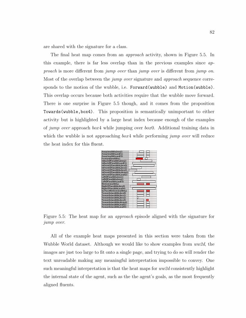
82

are shared with the signature for a class.

The final heat map comes from an approach activity, shown in Figure 5.5. In

this example, there is far less overlap than in the previous examples since ap-

proach is more different from jump over than jump over is different from jump on.

Most of the overlap between the jump over signature and approach sequence corre-

sponds to the motion of the wubble, i.e. Forward(wubble) and Motion(wubble).

This overlap occurs because both activities require that the wubble move forward.

There is one surprise in Figure 5.5 though, and it comes from the proposition

Towards(wubble,box4). This proposition is semantically unimportant to either

activity but is highlighted by a large heat index because enough of the examples

of jump over approach box4 while jumping over box0. Additional training data in

which the wubble is not approaching box4 while performing jump over will reduce

the heat index for this fluent.

Figure 5.5: The heat map for an approach episode aligned with the signature forjump over.

All of the example heat maps presented in this section were taken from the

Wubble World dataset. Although we would like to show examples from ww2d, the

images are just too large to fit onto a single page, and trying to do so will render the

text unreadable making any meaningful interpretation impossible to convey. One

such meaningful interpretation is that the heat maps for ww2d consistently highlight

the internal state of the agent, such as the the agent’s goals, as the most frequently

aligned fluents.

83

5.4 Recognition

In Chapter 4, we introduced a way to recognize activities as they occur by construct-

ing a finite state machine (FSM) with states and transitions that match the training

data. Signatures provided a way to selectively ignore some fluents and propositions

and allows the FSM to generalize to unseen episodes of an activity. We present

an experiment in which the FSMs described in Section 4.4.1 are used to recognize

activities. The experiment demonstrates that the FSMs from Section 4.4.1 have

higher recognition performance than FSMs induced directly from the training data.

The recognition task involves building a recognizer for each activity from training

episodes. The remaining episodes, which are not part of the training set, become test

episodes, and are “played” back to each FSM recognizer. Playing an episode involves

constructing the appropriate state for each moment in time during the episode and

updating the FSM accordingly. The recognizer either accepts or rejects the test

episode. We measure three different values: true positives, false positives, and true

negatives. True positives (tp) occur when a recognizer correctly accepts an episode.

A false positive (fp) occurs when a recognizer accepts an episode with a different

activity label, and a false negative (fn) occurs when the recognizer incorrectly rejects

an episode. These values are used to compute precision, recall and the F-measure.

The precision of a recognizer is the the number of episodes correctly identified out of

the total number of episodes accepted by the recognizer, and given by the formula:

Precision =tp

tp+ fp.

A recognizer that only correctly accepts activities from its class will have a

precision score of 1. A recognizer that accepts many more activities than it should

will have a lower precision score, and precision scores range from 0 to 1. The recall

of a recognizer is the number of episodes correctly identified out of the total number

of episodes with the same class label, given by the formula:

Recall =tp

tp+ fn.

84

Intuitively a recognizer can get a high recall by accepting every test episode

hoping that it shares the same class label of the recognizer, but this will reduce

the precision of the recognizer. Like precision, recall can vary from 0 to 1. Last is

the F-measure (van Rijsbergen, 1979) which is the harmonic mean of precision and

recall and also varies between 0 and 1:

F-measure = 2× precision× recall

precision + recall.

Similar to classification, we perform a K-fold cross validation on the training

data from ww and ww2d. This time we choose three values of K in order to vary

the amount of training data, and thus affect what is learned by the signature. We

exclude everything from the signature not seen in at least 80% of the training data, so

if a signature is trained on 20 episodes, any tuples seen fewer than sixteen times are

excluded from alignment. This is a very aggressive exclusion rate, but by excluding

most of the lower frequency tuples away from the signature, we end up with a more

general FSM recognizer.

We found that for the most part none of the recognizers built from just the

training data ever accepted an episode that it had not been trained on. The excep-

tion to this is the FSM for approach because it is a simple activity that occurs as a

component of the other activities. Without accepting a single episode from the test

set we cannot calculate the precision, recall, or F-measure. So, instead we focus on

the results generated by the signature based FSMs, presented in Figure 5.6. On the

left hand side are the plots containing the F-measures for 2-fold, 6-fold, and 10-fold

cross validations.

Overall it looks as though signatures constructed from event sequences ordered by

end times of the fluents are the best at pruning the FSM recognizer, but signatures

trained on sequences of Allen relations have high F-measures across most of the

activities. One consistent activity across all the Wubble World data is approach. The

F-measure consistently seems to be between 0.2 and 0.4 regardless of the sequence

representation. Recall that the F-measure is the harmonic mean of precision and

recall. The recall for the approach FSM is consistently high, but the precision is

85

always very low because the approach activity is performed whenever we do any

of the other activities. All Wubble World activities involve approaching the box,

and they differ in the interactions with the box. So, the FSM is not necessarily

incorrect all of the time, but rather the other activities contain or are composed

from an approach activity. Viewing an activity as composed of simple activities is

an important ability of our system and we discuss possible extensions to handle

hierarchical activities in Chapter 7.

FSM recognizers constructed from signatures trained on Wubble World 2D ac-

tivities do not fare as well across the board. Across all of the representations 6-folds

seems to produce the highest consistent F-measure. It appears as though Allen se-

quences do pretty well, and for 6 folds most of the activities can be recognized with

F-measures around 0.8, which is very high.

In most of the representations, it does not appear as though more training data

is helping the signature prune the FSM in order to get better performance. There

are two ways to interpret this; first, signatures do not need many training instances

before they successfully select which fluents can be ignored, and second the FSM

recognizers can only perform so well on this task. We saw evidence that signa-

tures need relatively few training instances before doing pretty well in Section 5.2.4,

and in Chapter 7 we address potential shortcomings in the FSM representation by

proposing alternative representations and learning algorithms for constructing more

general recognizers.

5.5 Inferring Hidden State

The next experiment demonstrates how well signatures can be used to infer un-

observable relations, e.g. relations that involve motor commands or propositions

corresponding to internal cognitive state. We focus on sequences of Allen relations

because the highest classification accuracy for the CAVE classifier came from sig-

natures trained on Allen sequences. Signatures are built from sequences in which

all of the relations are observable. There are two parts to this experiment. First

86

Wubble World Wubble World 2D

Event (start) K-Folds

F-Measure

2 6 100.0

0.2

0.4

0.6

0.8

1.0

K-Folds

F-Measure

2 6 10

0.0

0.2

0.4

0.6

0.8

1.0

Event (end) K-Folds

F-Measure

2 6 10

0.0

0.2

0.4

0.6

0.8

1.0

K-Folds

F-Measure

2 6 10

0.0

0.2

0.4

0.6

0.8

1.0

Event (both) K-Folds

F-Measure

2 6 10

0.0

0.2

0.4

0.6

0.8

1.0

K-Folds

F-Measure

2 6 10

0.0

0.2

0.4

0.6

0.8

1.0

Allen K-Folds

F-Measure

2 6 10

0.0

0.2

0.4

0.6

0.8

1.0

K-Folds

F-Measure

2 6 10

0.0

0.2

0.4

0.6

0.8

1.0

pushrightleftapproachjump-onjump-over

ballchasecolumneatfightflee

Figure 5.6: Results of the recognition task. The F-measures for varying amounts oftraining.

we test how well CAVE can classify episodes in which some of the propositions are

unobservable. Second we test the signatures’ ability to infer unobservable relations

87

in the proper order from sequences in which they have been removed. This is a

precision test.

ww ww2dM SD M SD

Allen Sequence 95.40% 5.17 70.83% 13.18

Table 5.7: Classification performance when some of the propositions are unobserv-able.

Table 5.7 contains the classification accuracy of the CAVE classifier on a 10-fold

cross-validation of the ww and ww2d datasets. Prior to testing each episode was

stripped of unobservable propositions. In ww, the unobservable propositions cor-

respond to motor commands such as Jump(wubble) and Forward(wubble), and in

ww2d the unobservable propositions correspond to the goals of the agent as well as

the internal affective state of the agent, i.e. valence(agent), energy(agent) and

goal(agent). The performance on ww datasets is relatively unaffected by the ab-

sence of internal propositions, but on the ww2d datasets it is a much larger problem.

The signatures learned from the ww2d rely less on the environment variables, such

as positions and distances, and contain many more unobservable propositions. Even

though performance is affected, CAVE still performs above 70% accuracy.

The second part of the experiment is to see if the inferred relations from the

signature can correctly capture the affective state, assuming that the episode has

been classified correctly. We again use the cross-validation experiment design. We

build signatures for each activity in each fold when all propositions are observable.

From each signature we select the α = 10 most frequent relations that contain at

least one of the unobservable propositions as the inferred relations. We also preserve

the order that relations occur within the signature so that the inferred relations can

be treated just like a qualitative sequence. An example from the activity chase

is shown in Table 5.8. We can see that a large number of the inferred relations

correspond to the current goals and states of the agent. Some subset of the inferred

relations occur in each of the test sequences, so we measure the alignment between

88

the inferred relations and those in the test sequence. We expect that the most

overlap will come from sequences that match the activity the signature was trained

on.

Inferred Relations((novel(agent1 agent2) s (goal(agent1) PursueGoal))) 18(((goal(agent1) PursueGoal) c (distance(agent1 agent2) 1))) 18(((goal(agent1) PursueGoal) c (arousal(agent1) up))) 18(((goal(agent1) PursueGoal) c (distance(agent1 agent2) down))) 18(((goal(agent1) PursueGoal) c (energy(agent1) stable))) 18(((goal(agent1) PursueGoal) c (valence(agent1) stable))) 18(((state(agent1) charge) c (arousal(agent1) up))) 17(((state(agent1) charge) c (distance(agent1 agent2) down))) 17(((state(agent1) charge) c (energy(agent1) stable))) 17(((goal(agent1) PursueGoal) c (heading(agent2) up))) 17

Table 5.8: The top 10 inferred relations and their weights in the signature for chasetrained on qualitative sequences of Allen relations

Table 5.9 shows the results on the ww dataset and Table 5.10 contains the results

on the ww2d dataset. The cells in each table contain the average amount of overlap

between the most frequent relations in the signature and the actual hidden relations

that occur in each episode from the test set. On average, 90% of the inferred

relations from the jump on signature correspond to hidden relations in unseen jump

on episodes. This means that, in expectation, if the agent were to correctly classify

a jump on episode, then 90% of its inferred relations would be present in the episode.

What if the agent classifies an episode incorrectly? How will this affect the ac-

curacy of inferred relations? Tables 5.9 and 5.10 shows the accuracy of inferred

relations for all pairs of activities. Along the diagonal are cases where the classifica-

tion of the activity is accurate, off-diagonal cases are incorrectly classified episodes.

For example, if the agent classifies a push as an approach then only 51% of the

inferred hidden relations will actually occur in the episode. (The fact that there is

any overlap at all is due to the overlap between the activities: in both cases the

agent approaches the box.)

This experiment confirms that if the agent can correctly classify the activity of

89

Signaturesapproach push jump on jump over left right

approach 0.62 0.19 0.18 0.06 0.30 0.34push 0.51 1 0.17 0.14 0.35 0.42

jump on 0.48 0.30 0.90 0.85 0.36 0.34jump over 0.44 0.46 0.68 1 0.36 0.32

left 0.34 0.54 0.19 0.20 0.99 0.98right 0.32 0.58 0.18 0.20 0.98 0.99

Table 5.9: A matrix showing the percent overlap between the α most frequent hiddenrelations in the signature and the hidden relations that exist in the test set, but arenot observable in the ww dataset.

another agent, it can select the α most frequent relations as inferred hidden relations,

and they will be correct with high probability.

Signaturescolumn ball chase flee fight eat

column 0.97 0.81 0.00 0.01 0.23 0.13ball 0.18 0.97 0.00 0.01 0.16 0.13

chase 0.01 0.07 0.98 0.05 0.04 0.02flee 0.05 0.17 0 0.97 0.06 0.11fight 0.13 0.19 0.63 0.06 0.96 0.19eat 0 0.02 0 0.03 0 0.97

Table 5.10: A matrix showing the percent overlap between the α most frequenthidden relations in the signature and the hidden relations that exist in the test set,but are not observable for the ww2d dataset.

5.6 Wrapping Up

In this chapter we focused on two datasets generated from virtual worlds. We

showed that the CAVE algorithm can learn to classify and recognize activities with

high accuracy in both of these domains. The question remains though if this is

due to the representations and algorithms or because of the way that we encoded

the sensors in the virtual worlds. In the next chapter, we explore this question

90

more thoroughly, and argue that the performance is due to the representations and

algorithms and not specific to these virtual worlds.

91

CHAPTER 6

APPLICATIONS TO DATA MINING

The previous chapter demonstrates that the qualitative sequences and signature

learning methods perform well at a variety of tasks, such as classification, infer-

ence, and recognition. In this chapter we extend the experiments to determine how

well the sequences and signatures perform on other datasets. In all of the previous

chapters, the data captured activities that software agents could perform in simu-

lation. In this chapter we turn our attention to datasets generated from different

processes. Furthermore, in the descriptions of the representations and algorithms

there were unanswered questions. For instance, which of the two methods we use

to convert real-valued time series into symbolic time series contributes more to the

overall performance of the system. We address this question as well as others in this

chapter.

6.1 Datasets

In addition to the Wubble World datasets, all experiments are carried out on five

other times series datasets. We introduce the other datasets in order to show that

the methods outlined in previous chapters will generalize and the results we showed

in the previous chapter is not an artifact of the way we encoded the simulations.

Some of the datasets are unique to this dissertation, e.g. the handwriting datasets,

and the other are representative of real-world datasets. Other datasets were included

that had similar properties to our simulation data. First they had to be multivariate,

since our representations and learning algorithms rely on multivariate time series.

Second, each dataset should capture some “activity,” for example in the handwriting

data an activity occurs when the subject writes down a specific letter. An episode

corresponds to a specific example of the letter written by a single person. The final

92

HW1 HW2 HW3

Classes 26. 26. 26.Examples 21.00 23.00 21.96

Time 69.61 124.58 66.59Fluents 33.02 38.04 32.52Allen 304.76 389.23 310.35CBA 930.03 954.30 931.09

Table 6.1: Average values for the episodes in the handwriting datasets.

property that we looked for is that there is difference between episodes of the same

activity, i.e. every character written by a person is not exactly the same. Each of

the datasets outlined here have all of these properties.

6.1.1 Handwriting

We created this dataset by collecting writing samples from three different subjects.

Each subject, identified as HW1, HW2, and HW3, contributed at least twenty ex-

amples of each character in the alphabet. The data was collected from a Wacom

Intuos3 pen tablet with custom software that sampled the coordinate information

of the stylus at regular intervals. Position information cannot be recorded while the

pen is not in contact with the table, but we can record that the pen was picked

up and where it was placed down next. Stroke information is important during the

conversion from real-valued time series into our symbolic SDL language. The stroke

provides markers so that the first difference is calculated correctly on the dataset.

Table 6.1 contains the average number of examples and other specifics about the

dataset for each subject1.

The training data for each subject is treated individually and we train signatures

for each character, for each subject. This way the system learns to classify and

recognize a specific subject’s writing style.

1For HW3, we were unable to recorded one example of the character ’p’ as the result of user

error during data gathering.

93

Num Examples Time Num Fluents Allen CBAabnormal 67 74.78 54.34 866.99 3,199.52normal 133 87.95 62.95 917.53 3,361.83

Table 6.2: Average values for the episodes in the ecg dataset.

Num Examples Time Num Fluents Allen CBAabnormal 127 137.99 66.57 965.45 3,736.33normal 1067 129.89 60.30 817.71 2,754.36

Table 6.3: Average values for the episodes in the wafer dataset.

6.1.2 ECG

The electrocardiogram (ecg) dataset contains measurements of cardiac electrical ac-

tivity as recorded from two electrodes at standardized locations on the body during

a single heartbeat, called lead0 and lead1 (Olszewski, 2001). The dataset was an-

alyzed by a domain expert and a label of normal or abnormal was assigned to an

episode in the dataset. Abnormal heartbeats are representative of a cardiac pathol-

ogy known as supraventricular premature beat. Full details on how the dataset was

gathered can be found in (Olszewski, 2001). Table 6.2 contains the averages for each

label.

6.1.3 Wafer

The wafer (wafer) dataset is a collection of time series datasets containing measure-

ments from vacuum-chamber sensors during the etching process applied to a silicon

wafer during the manufacture of semiconductor microelectronics (Olszewski, 2001).

Like the ecg dataset, each sample was analyzed by a domain expert and given a label

of normal or abnormal. The average values for different features of the dataset are

shown in Table 6.3. There are many more normal episodes than there are abnormal

episodes in this dataset, but we shall see that it does not impact performance.

6.1.4 Japanese Vowel

This dataset was generated from nine male speakers uttering two Japanese vowels

/ae/ successively (Kudo et al., 1999). The time-series are variable length ranging

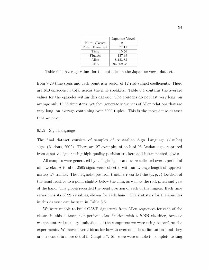
94

Japanese VowelNum. Classes 9.

Num. Examples 71.11Time 15.56

Fluents 137.39Allen 8,123.85CBA 295,862.28

Table 6.4: Average values for the episodes in the Japanese vowel dataset.

from 7-29 time steps and each point is a vector of 12 real-valued coefficients. There

are 640 episodes in total across the nine speakers. Table 6.4 contains the average

values for the episodes within this dataset. The episodes do not last very long, on

average only 15.56 time steps, yet they generate sequences of Allen relations that are

very long, on average containing over 8000 tuples. This is the most dense dataset

that we have.

6.1.5 Sign Language

The final dataset consists of samples of Australian Sign Language (Auslan)

signs (Kadous, 2002). There are 27 examples of each of 95 Auslan signs captured

from a native signer using high-quality position trackers and instrumented gloves.

All samples were generated by a single signer and were collected over a period of

nine weeks. A total of 2565 signs were collected with an average length of approxi-

mately 57 frames. The magnetic position trackers recorded the (x, y, z) location of

the hand relative to a point slightly below the chin, as well as the roll, pitch and yaw

of the hand. The gloves recorded the bend position of each of the fingers. Each time

series consists of 22 variables, eleven for each hand. The statistics for the episodes

in this dataset can be seen in Table 6.5.

We were unable to build CAVE signatures from Allen sequences for each of the

classes in this dataset, nor perform classification with a k-NN classifier, because

we encountered memory limitations of the computers we were using to perform the

experiments. We have several ideas for how to overcome these limitations and they

are discussed in more detail in Chapter 7. Since we were unable to complete testing

95

AuslanNum. Classes 95.

Num. Examples 27.00Time 47.29

Fluents 257.43Allen 24,594.60CBA 1,013,926.47

Table 6.5: Average values for the episodes in the Auslan dataset.

on this dataset, it is often left out of our analysis.

6.2 Classification

In this section we examine the performance of the representations and algorithms on

classification tasks. Experiments are performed on the two classifiers described in

Chapter 5, namely a k-NN classifier and a CAVE classifier. We split the classifiers

into separate sections because additional experiments are performed depending on

the classifier.

6.2.1 k-NN Classifier

We begin by establishing a baseline for each of our datasets. We perform the same

classification task, described in the previous chapter, on each dataset. The results

for a 10-fold cross validation are shown for 10-NN in Table 6.6. In general, classi-

fication accuracy is above 75%, and for the Wubble World, handwriting, and wafer

datasets we are performing well above 90% classification accuracy. The k-NN classi-

fier performs the worst on the vowel dataset which may be attributed to the density

of the data.

Based on the results in the Table 6.6, it does not appear to matter which rep-

resentation we construct a sequence from. For a given dataset, 10-NN performs

with roughly the same accuracy. This is confirmed with a two-way factorial analysis

of variance with repeated measures (Table 6.7). We chose to use a repeated mea-

sures design since each dataset was evaluated via a K-folds cross-validation (Cohen,

96

starts ends both Allen CBAM SD M SD M SD M SD M SD

ww 97.62 3.11 96.90 4.72 98.12 4.05 97.03 5.10ww2d 98.33 3.51 96.67 4.30 99.17 2.64 99.17 2.64HW1 98.27 1.42 97.63 1.76 98.53 1.21 97.88 1.91 96.99 2.12HW2 98.85 1.38 97.88 1.32 98.65 1.33 98.21 1.47 95.83 1.29HW3 96.67 2.80 96.92 2.15 96.79 1.71 94.61 2.38 92.23 2.62Auslan 84.07 1.76 80.25 2.23 84.88 2.22ecg 82.65 7.75 81.07 9.38 81.07 8.89 83.65 8.46 83.12 7.60wafer 97.15 2.03 96.99 1.54 97.40 1.88 97.74 1.27 97.57 0.84vowel 71.91 3.89 72.97 5.14 76.72 3.83 76.07 5.96

Table 6.6: Percent correct with a 10-NN classifier from a 10-fold cross validationclassification task.

1995)2.

Source df F p valueDataset 7 98.4444 < 0.0001Representation 3 0.1964 0.8989Dataset × Representation 21 0.3954 0.9967

Table 6.7: A two-way analysis of variance for dataset by representation shows onemain effect and no significant interaction effect.

The next thing to do is to place the results within some context. Table 6.8

contains the best published performance for datasets not constructed for this dis-

sertation. The k-NN classifier is outperformed in the Auslan and vowel datasets,

but performs as well or better on the ecg and wafer datasets.

Dataset Performance CitationAuslan 97.90% Kadous and Sammut (2005)vowel 96.50% Rodrıguez et al. (2005)ecg 70.97% Weng and Shen (2008)

wafer 98.64% Weng and Shen (2008)

Table 6.8: Best classification accuracy for several of our datasets.

In the previous chapter, we were able to show that classification on the Wubble

World datasets was not a challenging problem since we could shuffle the order of the

sequences and still perform quite well on the classification task. In Figure 6.1, we

2Auslan was not part of the analysis, nor was the CBA sequence representation.

97shuffling-anova By (activity, representation, fold) By (activity, representation): Graph BuilderPage 1 of 1

Representation

Allen both ends starts

Cla

ssifi

catio

n A

ccur

acy

(%)

0.1

0.2

0.3

0.4

0.5

0.6

0.7

0.8

0.9

1Legend

ecg

HW1

HW2

HW3

wafer

Graph Builder

Figure 6.1: Classification accuracy across activity by each representation after shuf-fling the sequences before training and testing.

see the classification accuracy of our k-NN classifier on each dataset after shuffling

the sequences prior to training and testing. For each dataset, the k-NN classifier is

still able to classify with high accuracy when it is trained on sequences of the Allen

relations. This is probably because Allen relations preserve order information, so

even after shuffling we can only match Allen relations if two propositions occurred

in the correct order in the same relationship. The k-NN classifier consistently per-

formed very poorly on the handwriting data. This is expected since it contains the

fewest variables (x and y) and each variable is guaranteed to occur in every episode

regardless of the character being written.

Ablation Study

In Chapter 3, we presented two methods for converting real-time time series into

symbolic time series. It was left as an open question which one of the two methods

contributes more to the classification accuracy. In this experiment we compare the

performance of our k-NN classifier in three different treatment conditions. The first

treatment is when the classifier is trained on episodes containing only SAX variables.

In the second treatment, the classifier is trained on episodes containing only SDL

variables. The final treatment condition and results are shown in Table 6.6. The

table contains the classification accuracy when both SAX and SDL variables are

98

present during training and testing. This type of experiment is sometimes called an

ablation experiment since we remove a component of the representation in order to

evaluate its role (Cohen, 1995).

The results after removing all SDL propositions are shown in Table 6.9, and

the results of removing the SAX variables are shown in Table 6.10. For the most

part, SAX appears to be contributing more to our classification accuracy than the

variables produced from the SDL conversion. Visually this can be confirmed by

Figure 6.2. The bar plots correspond to the difference in performance between the

k-NN classifier trained on sequences with both sets of variables and the performance

of the k-NN classifier with the SAX (or SDL) variables. Lower bars are better since

they represent a smaller difference in scores. The blue bars (corresponding to SAX

variables) are much smaller than the red bars for the handwriting datasets and

slightly smaller for the vowel datasets. This trend is reversed for the ecg dataset and

SDL has a smaller difference. In the wafer dataset both seem to contribute equally.

starts ends both AllenM SD M SD M SD M SD

HW1 98.08 2.87 97.37 2.10 97.88 2.79 96.09 3.36HW2 96.28 2.88 97.37 2.71 97.18 2.79 94.10 3.66HW3 96.47 2.48 96.02 2.00 96.60 2.58 93.52 2.16ecg 73.91 9.85 75.51 7.76 73.43 7.06 70.06 10.86wafer 95.73 1.01 95.73 1.01 95.73 1.01 96.81 1.25vowel 62.85 6.90 65.44 6.35 63.48 5.62 64.39 5.19

Table 6.9: Classification results for the k-NN classifier when only the variablesgenerated by the SAX process are available (SDL variables ablated).

We confirmed that SDL and SAX are significantly different with a three-way

analysis of variance with repeated measures. The classification accuracy was the

dependent variable and the factors were: the representation, the dataset, and the

conversion method (SAX, SDL, or SAX+SDL). We found two main effects of conver-

sion method and the dataset and a significant interaction effect between conversion

method and activity (Table 6.11). Figure 6.2 captures this. SAX performs signif-

icantly better than SDL on the handwriting and vowel datasets, but significantly

worse on the ecg datasets, hence the significant interaction effect. Using both SAX

99untitled 93: Graph Builder Page 1 of 1

Ablation Differences (Representation x Activity)

ecg HW1 HW2 HW3 vowel waferactivity

Representation

Allen both ends starts

Diff

eren

ce (%

)

-5

0

5

10

15

20

25

30

35

Allen both ends starts Allen both ends starts Allen both ends starts Allen both ends starts Allen both ends starts

Legend

SAX

SDL

Graph Builder

Figure 6.2: The difference in performance by representation and activity for thek-NN classifier trained with episodes containing both SAX and SDL variables con-trasted with the performance for the k-NN classifier trained with episodes containingonly SAX (or SDL) variables.

and SDL seems like the preferred way to go since that conversion method signifi-

cantly outperforms either method individually.

starts ends both AllenM SD M SD M SD M SD

HW1 69.42 4.75 71.35 6.44 70.32 4.17 66.99 4.53HW2 74.68 3.20 72.44 6.13 76.35 4.35 73.21 4.87HW3 65.39 6.37 65.72 4.70 66.23 5.86 63.15 6.09ecg 80.64 7.11 79.69 9.47 79.67 7.45 82.54 11.06wafer 95.90 1.69 95.23 1.25 96.40 1.68 97.99 1.45vowel 56.23 4.27 54.15 6.85 56.05 6.18 63.34 5.00

Table 6.10: Classification results for the k-NN classifier when only the variablesgenerated by the SDL process are available (SAX variables ablated).

6.2.2 CAVE

In this section we explore different facets of the CAVE algorithms. First we look at

CAVE performance on the classification task across multiple datasets, the results of

which are shown in Table 6.12. In all of the datasets we held the exclusion percentage

at 50% to establish a baseline. Recall that the exclusion percentage determines the

minimum weight values for tuples in the signature for inclusion. Effectively, the

exclusion percentage ignores low weight tuples without pruning them. The best

classification accuracy across all of the datasets comes from the CAVE classifier

trained on sequences of Allen relations. This is confirmed with a post-hoc analysis

100

Source df F p valueConversion Method 2 392.7431 < 0.0001Dataset 5 360.8100 0.0000Conversion Method × Activity 10 71.9144 < 0.0001Representation 3 0.1767 0.9123Conversion Method × Representation 6 0.5112 0.8003Dataset × Representation 15 1.1427 0.3110Conversion Method × Dataset × Representation 30 0.4204 0.9977

Table 6.11: A three-way analysis for the data shown in Figure 6.2.

on a two-way analysis of variance with repeated measures, the results of which are

shown in Table 6.13.

starts ends both Allen CBAM SD M SD M SD M SD M SD

ww 50.41% 14.01 82.89% 6.13 79.69% 9.37 98.89% 2.34ww2d 90.00% 6.57 87.50% 9.00 92.50% 6.15 95.00% 7.03HW1 93.21% 3.53 91.99% 3.94 91.73% 3.01 95.90% 2.25 92.37% 3.44HW2 79.17% 5.28 81.22% 7.66 80.90% 7.24 92.63% 4.28 82.24% 2.85HW3 76.82% 5.12 78.63% 4.29 80.93% 2.62 89.47% 3.33 88.96% 2.34Auslan 68.91% 2.46 61.16% 2.38 71.63% 2.38ecg 34.48% 4.57 37.48% 5.41 34.53% 2.88 61.99% 11.93 70.53% 9.83wafer 94.56% 2.58 94.22% 2.08 94.64% 3.06 91.11% 2.60vowel 39.97% 9.62 39.24% 3.61 41.36% 4.35 14.85% 6.49

Table 6.12: The classification results for the CAVE classifier on six different repre-sentations. Results are reported from a 10-fold cross validation classification task.

In general, the performance of the CAVE algorithm when trained on sequences

of Allen relations is worse than k-NN on the classification task. We will comment

more thoroughly on this in Section 6.3.

Source df F p valueDataset 5 171.9580 < 0.0001Representation 3 33.6624 < 0.0001Dataset × Representation 15 10.2374 < 0.001

Table 6.13: A two-way analysis of variance for dataset by representation shows twomain effects and a significant interaction effect.

101anova By (Exclude, Activity, Representation, fold) By (Exclude, Activity, Representation): Graph Builder Page 1 of 1

ecg HW1 HW2 HW3 wafer wwActivity

Exclude (%)

40 50 60 70 80 90

Cla

ssifi

catio

n A

ccur

acy

(%)

0.2

0.3

0.4

0.5

0.6

0.7

0.8

0.9

1

40 50 60 70 80 90 40 50 60 70 80 90 40 50 60 70 80 90 40 50 60 70 80 90 40 50 60 70 80 90

Legend

Allen

both

ends

starts

Graph Builder

Figure 6.3: Classification accuracy for each activity for different settings of theexclusion percentage.

Sensitivity

In this section we present two sensitivity analyses of the CAVE classifier. In the

first, we explore how classification accuracy changes as we modify the exclusion

percentage. We select seven values of the exclusion percentage and run the same

cross-validation task as before. Figure 6.3 contains the results of this experiment,

and demonstrates that it is not possible to select a single exclusion percentage that

will be optimal for all datasets and all representations. Selecting 50% to be the

exclusion percentage seems to be a consistent choice based on classification accuracy

across all activities for the Allen relations, which is confirmed by the analysis done

earlier in Table 6.13.

The second sensitivity analysis explores the relationship between the pruning

parameter and the time it takes to train a signature versus the performance of the

signature. In Chapter 4 we outlined a method to prune the signature during learning

in order to reduce the number of low frequency tuples in the signature. Pruning

works as follows: after updating the signature t times, all of the relations in the

signature with weights less than or equal to n are removed. In our experiment, we

set t = 10 and n = 3, meaning that the signature is pruned of all relations occurring

less than 4 times after a total of 10 training episodes. The signature is again pruned

after 20 training episodes, and so forth.

There are two conditions in this test. In the first condition, pruning is turned

102

off and the signature grows as large as necessary. In the The second condition the

signature is pruned during training. In both conditions, we measured the time it

takes to train a signature as well as the classification performance after training.

The results are shown in Table 6.14. Pruning saves a significant amount of time

during training without affecting performance.

Timingww HW1 HW2 HW3 ecg wafer

No Pruning 19750.88 91.44 124.47 104.23 12262.75 486858.05Pruning 8372.72 56.37 68.55 59.86 2288.15 28334.45

Performanceww HW1 HW2 HW3 ecg wafer

No Pruning 94.44 95.90 92.63 89.47 62.00 91.11Pruning 94.65 94.29 91.09 89.34 61.92 89.43

Table 6.14: The top part of the table contains the average number of millisecondsrequired to train a signature from sequences of Allen relations. The bottom partcontains the performance of the trained signatures in the two conditions.

6.3 Wrapping Up

There were a lot of results presented in this chapter so a recap is necessary. First

we found that both methods of classification perform well on our datasets and

real-world datasets generated by other authors. This result was tarnished slightly

because we found that classification on these datasets was not as difficult a task as

first envisioned. The classification accuracy of the k-NN classifier is independent of

the representation, therefore we can minimize the time spent in the k-NN classifier

by training it on event sequences rather than training it on relational sequences.

This is a surprising result considering that we found that Allen relations perform

significantly better than other relations for training signatures. In general, the k-NN

classifier outperforms the CAVE classifier on the datasets presented in this disser-

tation. If we were only interested in classification, then k-NN would be the obvious

choice since it performs better, but signatures do more than just classification, such

103

as inferring the hidden state and online recognition of activities. We answered the

question of which method for converting from real-valued time series into symbolic

time series is better for our applications, and it turns out that although SAX per-

forms better than SDL on more datasets, the one clear choice is to use both. Lastly,

the performance of the CAVE classifier is unaffected by pruning during training and

the amount of time spent training can be significantly reduced.

104

CHAPTER 7

CONCLUSIONS AND FUTURE WORK

The previous chapters describe novel representations and learning algorithms for

recognizing the activities that agents participate in and observe taking place. A

trained signature is able to identify when an activity occurs and can highlight what

parts of the corresponding time series are important observable or not. We also found

that signatures could be applied to more varied datasets that do not necessarily

include activities in which agents participate.

This work makes several contributions. Among them is a new sequence based

representation of multivariate time series. By transforming the time series into

sequences, we benefit from previous research with applications in everything from

biological sciences to natural language processing. We introduced two classes of

sequences, one based on events such as a propositional variable becoming true or

false and the other is based on the relationships between fluents.

Our work introduces a new aggregate structure called a signature that is useful

in a variety of tasks. Signatures are trained on qualitative sequences and capture

frequently occurring symbols in the sequence. When the sequences are constructed

from events, then the symbols are simply names of propositions, but when the

sequences are relational, then the symbol contains an Allen relation between two

fluents or a CBA between multiple fluents. The feature of signatures we explore most

in this dissertation is how it can be used as a classifier. We presented evidence that

the CAVE classifier, which is constructed from the signatures representing different

activities, performs very well at classification tasks, even in the absence of some

propositions. Furthermore, signatures provide a mechanism for inferring relations

and propositions that are only observable in certain occasions, for example, we

cannot access the internal state of another agent while watching them perform an

activity. Lastly, the signatures provide guidance on how to relax over-specified finite

105

state machines so that they can generalize to episodes not yet seen. Stored with

each signature is the original training episodes, and after pruning the signature, we

retain a subset of the original fluents for each episode, those that occur with the

most frequency. From the remaining fluents we construct a FSM that recognizes

episodes not yet seen.

7.1 Future Work

This dissertation presents important strides towards machine understanding of ac-

tivities in simulated environments. Furthermore, it posits a mechanism that would

allows an agent to reason about the intentions of other agents by using the premise

that the other agents would behave as it does. However, there is still much work

that needs to be done.

Currently we learn signatures of an activity in which all of the propositions are

grounded to a specific entity in the simulation. For example, every episode presented

as an example of the activity jump over contained the wubble interacting with the

exact same box in the simulation. So, the proposition Above(wubble,box0) corre-

sponds to precisely one box and currently, we would need to learn a different jump

over signature for each box. Arguably one of the most important areas for future

work is to develop signatures constructed from predicates instead of propositions.

This would be a huge benefit because it would allow us to learn a single signature

for the activity jump over and it would allow us to learn a different concept as well.

We could also learn about the set of objects that the agent can jump over.

Another issue is that signatures are an atomic unit. There does not exist a way

to describe an activity as a combination of multiple activities. For example, consider

the approach activity that caused most of our trouble in Chapter 5. Each ww activity

contained approach as a component to the activity and therefore each episode could

be classified or recognized as approach. An extension to this work is to determine

how signatures can be composed with other signatures in order to construct more

complex signatures, thus providing support for hierarchical activities.

106

In Chapter 6 we investigated the performance of methods for converting real-

valued time series into symbolic time series. We wanted to determine which allowed

us to perform better at classification tasks. We found that the inclusion of both con-

version methods resulted in the highest classification accuracy and that sometimes

one contributed more than the other. In some of the datasets SAX performed better

than SDL, and in others SDL performed better than SAX. The next step is to de-

termine what features of a dataset predict which of these representations will work

best. Additionally, these features may also help us predict performance as well. Re-

gardless, these two conversion methods are certainly not the only possibilities. We

mentioned that our time series do not conform to the assumptions of SAX, yet we

still perform well at classification tasks, so we need to evaluate other methods, like

Kohonen maps (Kohonen, 1995), and see if we can improve performance. Firoiu

and Cohen (1999) provide an additional method to “smooth” time series by fitting

lines piecewise to the time series. Further ablation experiments will determine the

affect on performance due to different conversion methods.

One of the most critical parts of the representations and algorithms is sequence

alignment. In this dissertation, we chose the brute force Needleman-Wunsch se-

quence alignment algorithm which stores a O(nm) table where m and n are the

lengths of the sequences (Needleman and Wunsch, 1970). One quick and necessary

enhancement is to develop the system around Hirschberg’s algorithm which can find

the optimal alignment in linear space (Hirschberg, 1975). More closely working with

computational biologists and researchers who regularly employ sequence algorithms

will help make the system overcome limitations on sequence length found in this

dissertation.

The algorithms presented that relax specialized FSMs in order to accept more

varied episodes can be improved. In general, finding a FSM with some small set

of states that agrees with all of the training data is a hard problem, known to

be NP-complete (Gold, 1978). So it remains to be seen how well we can do with

the generalized FSMs. In addition, we have not explored how to learn the FSM

transition probabilities in order to predict which states will come next. Transition

107

probabilities also provide a mechanism to estimate the probability of observing the

activity given the current state. Another area to be explored within the recognition

and our FSM representation is whether they can be used as part of the process that

infers the internal state of other agents. The benefit of moving the inference process

to the FSMs is that we can predict the current internal state of other agents as well

as future states. Right now, we can just retroactively look at an activity that occurs

and select a set of states that should have been true during the activity.

It has been observed that infants 14-15 months of age are more likely to imitate

intentional behaviors, and in some cases, having observed a failed action, the infants

will re-enact the successful version of the action if they have discerned the original

intent. It is unclear how our signatures/recognizers handle this type of scenario. In

terms of our FSM recognizers, we will develop a way to trigger when a recognizer

has almost completed and flag the time series as a failed attempt at the activity the

FSM is trained to recognize.

All of the training episodes for an activity contained just the activity and it

always executed to completion. How does the system behave when these assump-

tions are broken? For example, dogs often chase each other through the house, and

occasionally they stop mid chase by the water bowl in order to “refuel” before con-

tinuing the chase. In this episode, two separate activities occur and one interrupts

the other. None of our datasets contained this type of episodic structure, so first

we need to gather a dataset that does. Next we will train up signatures and see

if classification performance is affected, and examine how the sequence alignment

algorithm handles the interrupted activities.

7.2 Final Remarks

This dissertation represents an attempt to accomplish something that young chil-

dren do with relative ease, recognize what they are doing and what those around

them are doing. It is part of a shift in Artificial Intelligence, from highly trained

sophisticated systems that perform at levels equivalent to human experts on a sin-

108

gle task, but can do little else, to unsophisticated systems that do lots of different

things well, but is not an expert at any one task. This is one reason why we are not

concerned that the representation and algorithms presented in this dissertation do

not exceed the classification accuracy of every other algorithm in the field. These

representations and algorithms afford so much more than classification and that

makes them desirable.

109

REFERENCES

Agnew, Z. K., K. K. Bhakoo, and B. K. Puri (2007). The Human Mirror System:A Motor Resonance Theory of Mind-Reading. Brain research reviews, 54(2), pp.286–93.

Agrawal, R., G. Psaila, E. L. Wimmers, and M. Zaıt (1995). Querying Shapes ofHistories. Proceedings of the 21th International Conference on Very Large DataBases, pp. 502–514.

Agrawal, R. and R. Srikant (1994). Fast Algorithms for Mining Association Rules.In Proceedings of the 20th VLDB Conference.

Allen, J. F. (1983). Maintaining Knowledge About Temporal Intervals. Communi-cations of the ACM, 26(11), pp. 832–843.

Andre-Jonsson, H. and D. Z. Badal (1997). Using Signature Files for QueryingTime-Series Data. Lecture Notes in Computer Science, 1263, pp. 211–220.

Baker, C. L., R. Saxe, and J. B. Tenenbaum (2009). Action Understanding asInverse Planning. Cognition, 113(3), pp. 329–49.

Balasko, B., S. Nemeth, and J. Abonyi (2006). Qualitative Analysis of SegmentedTime-series by Sequence Alignment. In 7th International Symposium of Hungar-ian Researchers on Computational Intelligence. Budapest, Hungary.

Baldwin, D. A. and J. A. Baird (2001). Discerning Intentions in Dynamic HumanAction. Trends in Cognitive Sciences, 5, pp. 171–178.

Barrett, H., P. Todd, G. Miller, and P. Blythe (2005). Accurate Judgments of In-tention From Motion Cues Alone: A Cross-Cultural Study. Evolution and HumanBehavior, 26(4), pp. 313–331.

Batal, I., L. Sacchi, R. Bellazzi, and M. Hauskrecht (2009). Multivariate TimeSeries Classification with Temporal Abstractions. Florida Artificial IntelligenceResearch Society Conference.

Berndt, D. J. and J. Clifford (1994). Using Dynamic Time Warping to Find Patternsin Time Series. In AAAI-94 Workshop on Knowledge Discovery in Databases, pp.359–370.

Blythe, P. W., P. M. Todd, and G. F. Miller (1999). How Motion Reveals Intention:Categorizing Social Interactions. In Gigerenzer, G. and P. M. Todd (eds.) SimpleHeuristics That Make Us Smart, pp. 257–285. Oxford University Press, New York.

110

Bobick, A. F. and A. D. Wilson (1995). A State-Based Technique for the Sum-marization and Recognition of Gesture. In Proceedings of IEEE InternationalConference on Computer Vision, pp. 382–388.

Breazeal, C. (2003). Emotion and Sociable Humanoid Robots. International Journalof Human-Computer Studies, 59(1-2), pp. 119–155.

Breazeal, C., D. Buchsbaum, J. Gray, D. Gatenby, and B. Blumberg (2005). Learn-ing From and About Others: Towards Using Imitation to Bootstrap the SocialUnderstanding of Others by Robots. Artificial life, 11(1-2), pp. 31–62.

Buzan, D., S. Sclaroff, and G. Kollios (2004). Extraction and Clustering of MotionTrajectories in Video. In Proceedings of the 17th International Conference onPattern Recognition, 2004. ICPR 2004., pp. 521–524.

Chhieng, V. M. and R. K. Wong (2007). Adaptive Distance Measurement for TimeSeries Databases. In DASFAA, pp. 598–610.

Cohen, P. R. (1995). Empirical Methods for Artificial Intelligence. MIT Press.

Cohen, P. R. (2001). Fluent Learning: Elucidating the Structure of Episodes. Ad-vances in Intelligent Data Analysis, pp. 268–277.

Cohen, P. R., C. Sutton, and B. Burns (2002). Learning Effects of Robot Ac-tions using Temporal Associations. International Conference on Developmentand Learning.

Corkill, D. D. (1991). Blackboard Systems. AI Expert, 6(9), pp. 40–47.

Crick, C., M. Doniec, and B. Scassellati (2007). Who is IT? Inferring Role and Intentfrom Agent Motion. In Proceedings of the 6th IEEE International Conference onDevelopment and Learning, pp. 134–139.

Crick, C. and B. Scassellati (2008). Inferring Narrative and Intention from Play-ground Games. In Proceedings of the 7th IEEE Conference on Development andLearning, pp. 13–18.

Crick, C. and B. Scassellati (2010). Controlling a Robot with Intention Derivedfrom Motion. Topics in Cognitive Science, 2(1), pp. 114–126.

de Carvalho Junior, S. A. (2002). Sequence Alignment Algorithms. Master’s thesis,King’s College London.

Devisscher, M., B. D. Baets, I. Nopens, P. Control, J. Decruyenaere, and D. Benoit(2008). Pattern Discovery in Intensive Care Data Through Sequence Alignment ofQualitative Trends Data : Proof of Concept on a Diuresis Data Set. In Proceedings

111

of the ICML/UAI/COLT 2008 Workshop on Machine Learning for Health-CareApplications.

Dudani, S. A. (1976). The Distance-Weighted k-Nearest-Neighbor Rule. IEEETrans. Systems, Man, Cybernetics, 6(4), pp. 325–327.

Firoiu, L. and P. R. Cohen (1999). Abstracting from Robot Sensor Data usingHidden Markov Models. In Proceedings of the Sixteenth International Conferenceon Machine Learning, pp. 106–114.

Fleischman, M., P. Decamp, and D. K. Roy (2006). Mining Temporal Patterns ofMovement for Video Content Classification. Proceedings of the 8th ACM SIGMMInternational Workshop on Multimedia Information Retrieval.

Fu, A. W.-C., E. Keogh, L. Y. H. Lau, C. A. Ratanamahatana, and R. C.-W. Wong(2008). Scaling and time warping in time series querying. The VLDB Journal,17(4), pp. 899–921.

Galushka, M., D. Patterson, and N. Rooney (2006). Temporal Data Mining forSmart Homes. LNAI, 4008, pp. 85 – 108.

Gold, E. M. (1978). Complexity of Automaton Identification from Given Data.Information and Control, 37(3), pp. 302–320.

Großmann, A., M. Wendt, and J. Wyatt (2003). A Semi-supervised Method forLearning the Structure of Robot Environment Interactions. Lecture Notes inComputer Science, 2779, pp. 36–47.

Hastie, T., R. Tibshirani, and J. Friedman (2001). The Elements of StatisticalLearning. Springer.

Heider, F. and M. Simmel (1944). An Experimental Study of Apparent Behavior.The American Journal of Psychology, 57(2), p. 243.

Hirschberg, D. S. (1975). A Linear Space Algorithm for Computing Maximal Com-mon Subsequences. Communications of the ACM, 18(6), pp. 341–343.

Hoppner, F. (2001a). Discovery of Temporal Patterns - Learning Rules about theQualitative Behaviour of Time Series. In Proc. of the 5th European Conferenceon Principles and Practice of Knowledge Discovery in Databases, pp. 192 – 203.Springer, Freiburg, Germany.

Hoppner, F. (2001b). Learning Temporal Rules from State Sequences. Proceedingsof IJCAI Workshop on Learning from Temporal and Spatial Data, pp. 25–31.

112

Hoppner, F. and F. Klawonn (2002). Finding informative rules in interval sequences.Intelligent Data Analysis, 6, pp. 237–255.

Iacoboni, M., I. Molnar-Szakacs, V. Gallese, G. Buccino, J. C. Mazziotta, andG. Rizzolatti (2005). Grasping the Intentions of Others with One’s Own Mir-ror Neuron System. PLoS biology, 3(3), p. e79.

Just, W. (2001). Computational Complexity of Multiple Sequence Alignment withSP-Score. Journal of Computational Biology, 8(6), pp. 615–623.

Kadous, M. W. (2002). Temporal Classification: Extending the ClassificationParadigm to Multivariate Time Series. Ph.d., The University of New South Wales.

Kadous, M. W. and C. Sammut (2005). Classification of Multivariate Time Seriesand Structured Data Using Constructive Induction. Machine Learning, 58(2-3),pp. 179–216.

Kalman, R. E. (1960). A New Approach to Linear Filtering and Prediction Problems.Journal of Basic Engineering, 82(1), pp. 35–45.

Kam, P.-s. and A. W.-c. Fu (2000). Discovering Temporal Patterns for Interval-basedEvents. Lecture Notes in Computer Science, 1874, pp. 317–326.

Keogh, E. J. and M. J. Pazzani (2001). Derivative Dynamic Time Warping. InSIAM International Conference on Data Mining.

Kerr, W., P. Cohen, and Y.-h. Chang (2008). Learning and Playing in WubbleWorld. In Proceedings of the Fourth Artificial Intelligence and Interactive DigitalEntertainment Conference, pp. 66–71.

Kohonen, T. (1995). Self Organizing Maps. Springer.

Kudo, M., J. Toyama, and M. Shimbo (1999). Multidimensional Curve Classificationusing Passing-Through Regions. Pattern Recognition Letters, 20(11-13), pp. 1103–1111.

Lee, C. and Y. Xu (1996). Online, Interactive Learning of Gestures for Hu-man/Robot Interfaces. In Proceedings of IEEE International Conference onRobotics and Automation, April, pp. 2982–2987. IEEE.

Liao, T. W. (2005). Clustering of Time Series Data - A Survey. Pattern Recognition,38, pp. 1857–1874.

Lin, J., E. Keogh, S. Lonardi, and B. Chiu (2003). A Symbolic Representation ofTime Series, with Implications for Streaming Algorithms. DMKD ’03, pp. 2–11.

113

Lin, J., E. Keogh, L. Wei, and S. Lonardi (2007). Experiencing SAX: a NovelSymbolic Representation of Time Series. Data Mining and Knowledge Discovery,15, pp. 107–144.

Masuch, M., K. Hartman, and G. Schuster (2006). Emotional Agents for InteractiveEnvironments. In Fourth International Conference on Creating, Connecting andCollaborating through Computing (C5’06), pp. 96–102.

Mitsa, T. (2010). Temporal Data Mining. Chapman & Hall / CRC.

Morse, M. D. and J. M. Patel (2007). An Efficient and Accurate Method for Evalu-ating Time Series Similarity. In Proceedings of the 2007 ACM SIGMOD interna-tional conference on Management of data - SIGMOD ’07, p. 569. ACM Press.

Nathan, K., H. Beigi, G. Clary, and H. Maruyama (1995). Real-Time On-Line Un-constrained Handwriting Recognition Using Statistical Methods. In 1995 Inter-national Conference on Acoustics, Speech, and Signal Processing, pp. 2619–2622.

Needleman, S. B. and C. D. Wunsch (1970). A General Method Applicable to theSearch for Similarities in the Amino Acid Sequence of Two Proteins. Journal ofmolecular biology, 48(3), pp. 443–453.

Newtson, D. (1973). Attribution and the Unit of Perception of Ongoing Behavior.Journal of Personality and Social Psychology, 28(1), pp. 28–38.

Oates, T., L. Firoiu, and P. R. Cohen (1999). Clustering Time Series with HiddenMarkov Models and Dynamic Time Warping. In IJCAI-99 Workshop on SequenceLearning, pp. 17–21.

Oates, T., M. D. Schmill, and P. R. Cohen (2000). A Method for Clustering theExperiences of a Mobile Robot that Accords with Human Judgments. In AAAI-00.

Olszewski, R. (2001). Generalized Feature Extraction for Structural Pattern Recog-nition in Time-Series Data. Ph.D. thesis, Carnegie Mellon University.

Papapetrou, P., G. Kollios, S. Sclaroff, and D. Gunopulos (2009). Mining FrequentArrangements of Temporal Intervals. Knowl Inf Syst, pp. 1–39.

Pautler, D., B. Koenig, B.-k. Quek, and A. Ortony (2009). Inferring Intention andCausality from 2D Animations. Submitted.

Rodrıguez, J. J., C. J. Alonso, and J. A. Maestro (2005). Support Vector Machines ofInterval-Based Features for Time Series Classification. Knowledge-Based Systems,18, pp. 171–178.

114

Rosenstein, M. T. and P. R. Cohen (1999). Continuous Categories for a MobileRobot. Proceedings of the Sixteenth National Conference on Artificial Intelligence,pp. 634–640.

Sakoe, H. and S. Chiba (1978). Dynamic Programming Algorithm Optimization forSpoken Word Recognition. IEEE Transactions on Acoustics, Speech and SignalProcessing, 26(1), pp. 43–49.

Starner, T. E. (1995). Visual Recognition of American Sign Language Using HiddenMarkov Models. Ph.D. thesis, Massachusetts Institute of Technology.

Tukey, J. W. (1977). Exploratory Data Analysis. Addison-Wesley.

van Rijsbergen, C. J. (1979). Information Retrieval. University of Glasgow.

Vlachos, M., D. Gunopoulos, and G. Kollios (2002). Discovering Similar Multidi-mensional Trajectories. In 18th International Conference on Data Engineering(ICDE’02), pp. 673–684. San Jose, California.

Vlachos, M., M. Hadjieleftheriou, D. Gunopulos, and E. Keogh (2006). IndexingMultidimensional Time-Series. The VLDB Journal, 15(1), pp. 1–20.

Wang, L. and T. Jiang (1994). On the Complexity of Multiple Sequence Alignment.Journal of Computational Biology, 1(4), pp. 337–348.

Wang, Q., V. Megalooikonomou, and G. Li (2005). A symbolic representation of timeseries. In Proceedings of the Eighth International Symposium on Signal Processingand Its Applications, pp. 655–658.

Weng, X. and J. Shen (2008). Classification of Multivariate Time Series using Two-Dimensional Singular Value Decomposition. Knowledge-Based Systems, 21(7),pp. 535–539.

Winarko, E. and J. F. Roddick (2007). ARMADA – An Algorithm for DiscoveringRicher Relative Temporal Association Rules from Interval-Based Data. Data &Knowledge Engineering, 63, pp. 76–90.

Wu, S.-Y. and Y.-L. Chen (2009). Discovering Hybrid Temporal Patterns fromSequences Consisting of Point- and Interval-Based Events. Data & KnowledgeEngineering, 68(11), pp. 1309–1330.

Wu, X., V. Kumar, J. R. Quinlan, J. Ghosh, Q. Yang, H. Motoda, G. J. McLachlan,A. Ng, B. Liu, P. S. Yu, Z.-H. Zhou, M. Steinbach, D. J. Hand, and D. Steinberg(2008). Top 10 Algorithms in Data Mining. Knowledge and Information Systems,14(1), pp. 1–37.

115

Yang, K. and C. Shahabi (2004). A PCA-Based Similarity Measure for MultivariateTime Series. In Proc. Second ACM Int’l Workshop Multimedia Databases, pp.65–74.

Yang, K. and C. Shahabi (2007). An Efficient k Nearest Neighbor Search for Mul-tivariate Time Series. Information and Computation, 205(1), pp. 65–98.