Learning to Learn How to Learn: Self-Adaptive Visual Navigation using Meta-Learning Mitchell Wortsman 1 , Kiana Ehsani 2 , Mohammad Rastegari 1 , Ali Farhadi 1,2 , Roozbeh Mottaghi 1 1 PRIOR @ Allen Institute for AI, 2 University of Washington Abstract Learning is an inherently continuous phenomenon. When humans learn a new task there is no explicit distinc- tion between training and inference. As we learn a task, we keep learning about it while performing the task. What we learn and how we learn it varies during different stages of learning. Learning how to learn and adapt is a key property that enables us to generalize effortlessly to new settings. This is in contrast with conventional settings in machine learning where a trained model is frozen during inference. In this paper we study the problem of learn- ing to learn at both training and test time in the context of visual navigation. A fundamental challenge in naviga- tion is generalization to unseen scenes. In this paper we propose a self-adaptive visual navigation method (SAVN) which learns to adapt to new environments without any ex- plicit supervision. Our solution is a meta-reinforcement learning approach where an agent learns a self-supervised interaction loss that encourages effective navigation. Our experiments, performed in the AI2-THOR framework, show major improvements in both success rate and SPL for visual navigation in novel scenes. Our code and data are available at: https://github.com/allenai/savn. 1. Introduction Learning is an inherently continuous phenomenon. We learn further about tasks that we have already learned and can learn to adapt to new environments by interacting in these environments. There is no hard boundary between the training and the testing phases while we are learning and performing tasks: we learn as we perform. This stands in stark contrast with many modern deep learning techniques, where the network is frozen during inference. What we learn and how we learn it varies during differ- ent stages of learning. To learn a new task we often rely on explicit external supervision. After learning a task, we further learn as we adapt to new settings. This adaptation does not necessarily need explicit supervision; we often do this via interaction with the environment. Figure 1. Traditional navigation approaches freeze the model dur- ing inference (top row); this may result in difficulties generaliz- ing to unseen environments. In this paper, we propose a meta- reinforcement learning approach for navigation, where the agent learns to adapt in a self-supervised manner (bottom row). In this example, the agent learns to adapt itself when it collides with an object once and acts correctly afterwards. In contrast, a standard solution (top row) makes multiple mistakes of the same kind when performing the task. In this paper, we study the problem of learning to learn and adapt at both training and test time in the context of visual navigation; one of the most crucial skills for any vi- sually intelligent agent. The goal of visual navigation is to move towards certain objects or regions of an environment. A key challenge in navigation is generalizing to a scene that has not been observed during training, as the structure of the scene and appearance of objects are unfamiliar. In this paper we propose a self-adaptive visual navigation (SAVN) model which learns to adapt during inference without any explicit supervision using an interaction loss (Figure 1). Formally, our solution is a meta-reinforcement learn- ing approach to visual navigation, where an agent learns to adapt through a self-supervised interaction loss. Our approach is inspired by gradient based meta-learning al- gorithms that learn quickly using a small amount of data [13]. In our approach, however, we learn quickly using a 6750

Welcome message from author
This document is posted to help you gain knowledge. Please leave a comment to let me know what you think about it! Share it to your friends and learn new things together.
Transcript
Learning to Learn How to Learn:
Self-Adaptive Visual Navigation using Meta-Learning
Mitchell Wortsman1, Kiana Ehsani2, Mohammad Rastegari1, Ali Farhadi1,2, Roozbeh Mottaghi1
1 PRIOR @ Allen Institute for AI, 2 University of Washington
Abstract
Learning is an inherently continuous phenomenon.
When humans learn a new task there is no explicit distinc-
tion between training and inference. As we learn a task,
we keep learning about it while performing the task. What
we learn and how we learn it varies during different stages
of learning. Learning how to learn and adapt is a key
property that enables us to generalize effortlessly to new
settings. This is in contrast with conventional settings in
machine learning where a trained model is frozen during
inference. In this paper we study the problem of learn-
ing to learn at both training and test time in the context
of visual navigation. A fundamental challenge in naviga-
tion is generalization to unseen scenes. In this paper we
propose a self-adaptive visual navigation method (SAVN)
which learns to adapt to new environments without any ex-
plicit supervision. Our solution is a meta-reinforcement
learning approach where an agent learns a self-supervised
interaction loss that encourages effective navigation. Our
experiments, performed in the AI2-THOR framework, show
major improvements in both success rate and SPL for visual
navigation in novel scenes. Our code and data are available
at: https://github.com/allenai/savn.
1. Introduction
Learning is an inherently continuous phenomenon. We
learn further about tasks that we have already learned and
can learn to adapt to new environments by interacting in
these environments. There is no hard boundary between the
training and the testing phases while we are learning and
performing tasks: we learn as we perform. This stands in
stark contrast with many modern deep learning techniques,
where the network is frozen during inference.
What we learn and how we learn it varies during differ-
ent stages of learning. To learn a new task we often rely
on explicit external supervision. After learning a task, we
further learn as we adapt to new settings. This adaptation
does not necessarily need explicit supervision; we often do
this via interaction with the environment.
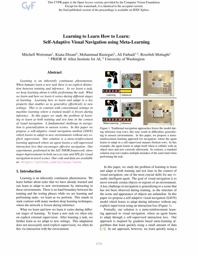
Figure 1. Traditional navigation approaches freeze the model dur-
ing inference (top row); this may result in difficulties generaliz-
ing to unseen environments. In this paper, we propose a meta-
reinforcement learning approach for navigation, where the agent
learns to adapt in a self-supervised manner (bottom row). In this
example, the agent learns to adapt itself when it collides with an
object once and acts correctly afterwards. In contrast, a standard
solution (top row) makes multiple mistakes of the same kind when
performing the task.
In this paper, we study the problem of learning to learn
and adapt at both training and test time in the context of
visual navigation; one of the most crucial skills for any vi-
sually intelligent agent. The goal of visual navigation is to
move towards certain objects or regions of an environment.
A key challenge in navigation is generalizing to a scene that
has not been observed during training, as the structure of
the scene and appearance of objects are unfamiliar. In this
paper we propose a self-adaptive visual navigation (SAVN)
model which learns to adapt during inference without any
explicit supervision using an interaction loss (Figure 1).
Formally, our solution is a meta-reinforcement learn-
ing approach to visual navigation, where an agent learns
to adapt through a self-supervised interaction loss. Our
approach is inspired by gradient based meta-learning al-
gorithms that learn quickly using a small amount of data
[13]. In our approach, however, we learn quickly using a
6750
small amount of self-supervised interaction. In visual navi-
gation, adaptation is possible without access to any reward
function or positive example. As the agent trains, it learns
a self-supervised loss that encourages effective navigation.
During training, we encourage the gradients induced by the
self-supervised loss to be similar to those we obtain from
the supervised navigation loss. The agent is therefore able
to adapt during inference when explicit supervision is not
available.
In summary, during both training and testing, the agent
modifies its network while performing navigation. This
approach differs from traditional reinforcement learning
where the network is frozen after training, and contrasts
with supervised meta-learning as we learn to adapt to new
environments during inference without access to rewards.
We perform our experiments using the AI2-THOR [23]
framework. The agent aims to navigate to an instance of
a given object category (e.g., microwave) using only vi-
sual observations. We show that SAVN outperforms the
non-adaptive baseline in terms of both success rate (40.8
vs 33.0) and SPL (16.2 vs 14.7). Moreover, we demonstrate
that learning a self-supervised loss provides improvement
over hand-crafted self-supervised losses. Additionally, we
show that our approach outperforms memory-augmented
non-adaptive baselines.
2. Related Work
Deep Models for Navigation. Traditional navigation meth-
ods typically perform planning on a given map of the
environment or build a map as the exploration proceeds
[26, 40, 21, 24, 9, 4]. Recently, learning-based navigation
methods (e.g., [50, 15, 27]) have become popular as they
implicitly perform localization, mapping, exploration and
semantic recognition end-to-end.
Zhu et al. [50] address target-driven navigation given a
picture of the target. A joint mapper and planner has been
introduced by [15]. [27] use auxiliary tasks such as loop
closure to speed up RL training for navigation. We differ
in our approach as we adapt dynamically to a novel scene.
[37] propose the use of topological maps for the task of
navigation. They explore the test environment for a long
period to populate the memory. In our work, we learn to
navigate without an exploration phase. [20] propose a self-
supervised deep RL model for navigation. However, no
semantic information is considered. [31] learn navigation
policies based on object detectors and semantic segmenta-
tion modules. We do not rely on heavily supervised detec-
tors and learn from a limited number of examples. [46, 44]
incorporate semantic knowledge to better generalize to un-
seen scenarios. Both of these approaches dynamically up-
date their manually defined knowledge graphs. However,
our model learns which parameters should be updated dur-
ing navigation and how they should be updated. Learning-
based navigation has been explored in the context of other
applications such as autonomous driving (e.g., [7]), map-
based city navigation (e.g., [5]) and game play (e.g., [43]).
Navigation using language instructions has been explored
by various works [3, 6, 17, 47, 29]. Our goal is different
since we focus on using meta-learning to more effectively
navigate new scenes using only the class label for the target.
Meta-learning. Meta-learning, or learning to learn, has
been a topic of continued interest in machine learning re-
search [41, 38]. More recently, various meta-learning tech-
niques have pushed the state of the art in low-shot problems
across domains [13, 28, 12].
Finn et al. [13] introduce Model Agnostic Meta-
Learning (MAML) which uses SGD updates to adapt
quickly to new tasks. This gradient based meta-learning ap-
proach may also be interpreted as learning a good parameter
initialization such that the network performs well after only
a few gradient updates. [25] and [48] augment the MAML
algorithm so that it uses supervision in one domain to adapt
to another. Our work differs as we do not use supervision
or labeled examples to adapt.
Xu et al. [45] use meta-learning to significantly speed up
training by encouraging exploration of the state space out-
side of what the actor’s policy dictates. Additionally, [14]
use meta-learning to augment the agent’s policy with struc-
tured noise. At inference time, the agent is able to better
adapt from a few episodes due to the variability of these
episodes. Our work instead emphasizes self-supervised
adaptation while executing a single visual navigation task.
Neither of these works consider this domain.
Clavera et al. [8] consider the problem of learning to
adapt to unexpected perturbations using meta-learning. Our
approach is similar as we also consider the problem of
learning to adapt. However, we consider the problem of
visual navigation and adapt via a self-supervised loss.
Both [18] and [48] learn an objective function. However,
[18] use evolutionary strategies instead of meta-learning.
Our approach for learning a loss is inspired by and simi-
lar to [48]. However, we adapt in the same domain without
explicit supervision while they adapt across domains using
a video demonstration.
Self-supervision. Different types of self-supervision have
been explored in the literature [1, 19, 11, 42, 49, 36, 34, 32].
Some works aim to maximize the prediction error in the rep-
resentation of future states [33, 39]. In this work, we learn
a self-supervised objective which encourages effective nav-
igation.
3. Adaptive Navigation
In this section, we begin by formally presenting the task
and our base model without adaptation. We then explain
how to incorporate adaptation and perform training and test-
ing in this setting.
6751
LSTM
Turn
Left
Look
Down
Move
Forward
…
Image
Feature
ResNet18 (Frozen)Current
observation
Glove Embedding
1×"## FC
Tile
$ = #
Concatenated
policy and
hidden states
&×(()* + ,)
()*×.×. ,/×.×.
,/×.×.
Laptop
Target
Object Class
$ = )
$ = *
Navigation-Gradient (Training only)
Forward Pass
Interaction-Gradient (Training and Inference)
Pointwise
Conv
Pointwise
Conv
1D Temporal
Conv
LSTM LSTM
01 2$
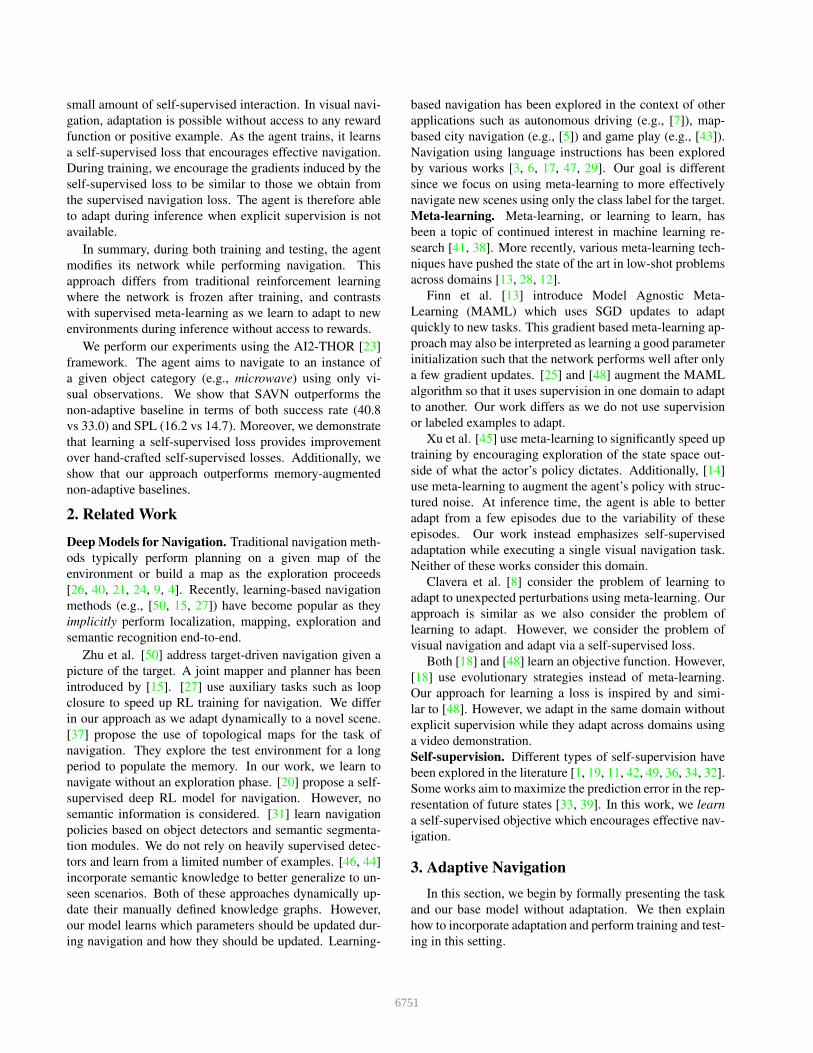
Figure 2. Model overview. Our network optimizes two objective functions, 1) self-supervised interaction loss Lφint and 2) navigation loss
Lnav. The inputs to the network at each time t are the egocentric image from the current location and word embedding of the target object
class. The network outputs a policy πθ(st). During training, the interaction and navigation-gradients are back-propagated through the
network, and the parameters of the self-supervised loss are updated at the end of each episode using navigation-gradients. At test time the
parameters of the interaction loss remain fixed while the rest of the network is updated using interaction-gradients. Note that the green
color in the figure represents the intermediate and final outputs.
3.1. Task Definition
Given a target object class, e.g. microwave, our goal is
to navigate to an instance of an object from this class using
only visual observations.
Formally, we consider a set of scenes S = {S1, ..., Sn}and target object classes O = {o1, ..., om}. A task τ ∈ Tconsists of a scene S, target object class o ∈ O, and initial
position p. We therefore denote each task τ by the tuple
τ = (S, o, p). We consider disjoint sets of scenes for the
training tasks Ttrain and testing tasks Ttest. We refer to the
trial of a navigation task as an episode.
The agent is required to navigate using only the egocen-
tric RGB images and the target object class (the target object
class is given as a Glove embedding [35]). At each time t
the agent takes an action a from the action set A until the
termination action is issued by the agent. We consider an
episode to be successful if, within certain number of steps,
the agent issues a termination action when an object from
the given target class is sufficiently close and visible. If
a termination action is issued at any other time, then the
episode concludes and the agent has failed.
3.2. Learning
Before we discuss our self-adaptive approach we begin
with an overview of our base model and discuss deep rein-
forcement learning for navigation in a traditional sense.
We let st, the egocentric RGB image, denote the agent’s
state at time t. Given st and the target object class, the net-
work (parameterized by θ) returns a distribution over the
actions which we denote πθ(st) and a scalar vθ(st). The
distribution πθ(st) is referred to as the agent’s policy while
vθ(st) is the value of the state. Finally, we let π(a)θ (st) de-
note the probability that the agent chooses action a.
We use a traditional supervised actor-critic navigation
loss as in [50, 27] which we denote Lnav. By minimiz-
ing Lnav, we maximize a reward function that penalizes the
agent for taking a step while incentivizing the agent to reach
the target. The loss is a function of the agent’s policies, val-
ues, actions, and rewards throughout an episode.
The network architecture is illustrated in Figure 2. We
use a ResNet18 [16] pretrained on ImageNet [10] to extract
a feature map for a given image. We then obtain a joint
feature-map consisting of both image and target information
and perform a pointwise convolution. The output is then
flattened and given as input to a Long Short-Term Memory
network (LSTM). For the remainder of this work we refer to
the LSTM hidden state and agent’s internal state represen-
tation interchangeably. After applying an additional linear
layer we obtain the policy and value. In Figure 2 we do not
show the ReLU activations we use throughout, or reference
the value vθ(st).
3.3. Learning to Learn
In visual navigation there is ample opportunity for the
agent to learn and adapt by interacting with the environ-
ment. For example, the agent may learn how to handle ob-
stacles it is initially unable to circumvent. We therefore pro-
pose a method in which the agent learns how to adapt from
interaction. The foundation of our method lies in recent
works which present gradient based algorithms for learning
to learn (meta-learning).
Background on Gradient Based Meta-Learning. We rely
on the meta-learning approach detailed by the MAML algo-
rithm [13]. The MAML algorithm optimizes for fast adap-
tation to new tasks. If the distribution of training and test-
6752
ing tasks are sufficiently similar then a network trained with
MAML should quickly adapt to novel test tasks.
MAML assumes that during training we have access to a
large set of tasks Ttrain where each task τ ∈ Ttrain has a small
meta-training dataset Dtrτ and meta-validation set Dval
τ . For
example, in the problem of k-shot image classification, τ is
a set of image classes and Dtrτ contains k examples of each
class. The goal is then to correctly assign one of the class
labels to each image in Dvalτ . A testing task τ ∈ Ttest then
consists of unseen classes.
The training objective of MAML is given by
minθ
∑
τ∈Ttrain
L(
θ − α∇θL(
θ,Dtrτ
)
,Dvalτ
)
, (1)
where the loss L is written as a function of a dataset and
the network parameters θ. Additionally, α is the step size
hyper-parameter, and ∇ denotes the differential operator
(gradient). The idea is to learn parameters θ such that they
provide a good initialization for fast adaptation to test tasks.
Formally, Equation (1) optimizes for performance on Dvalτ
after adapting to the task with a gradient step on Dtrτ . In-
stead of using the network parameters θ for inference on
Dvalτ , we use the adapted parameters θ − α∇θL (θ,D
trτ ). In
practice, multiple SGD updates may be used to compute the
adapted parameters.
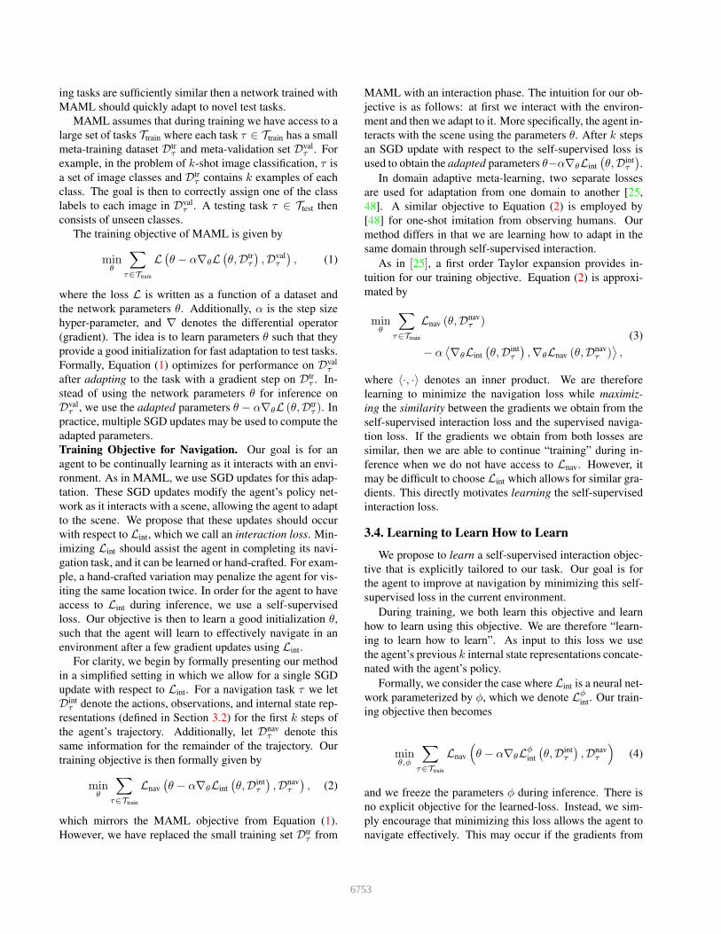
Training Objective for Navigation. Our goal is for an
agent to be continually learning as it interacts with an envi-
ronment. As in MAML, we use SGD updates for this adap-
tation. These SGD updates modify the agent’s policy net-
work as it interacts with a scene, allowing the agent to adapt
to the scene. We propose that these updates should occur
with respect to Lint, which we call an interaction loss. Min-
imizing Lint should assist the agent in completing its navi-
gation task, and it can be learned or hand-crafted. For exam-
ple, a hand-crafted variation may penalize the agent for vis-
iting the same location twice. In order for the agent to have
access to Lint during inference, we use a self-supervised
loss. Our objective is then to learn a good initialization θ,
such that the agent will learn to effectively navigate in an
environment after a few gradient updates using Lint.
For clarity, we begin by formally presenting our method
in a simplified setting in which we allow for a single SGD
update with respect to Lint. For a navigation task τ we let
Dintτ denote the actions, observations, and internal state rep-
resentations (defined in Section 3.2) for the first k steps of
the agent’s trajectory. Additionally, let Dnavτ denote this
same information for the remainder of the trajectory. Our
training objective is then formally given by
minθ
∑
τ∈Ttrain
Lnav
(
θ − α∇θLint
(
θ,Dintτ
)
,Dnavτ
)
, (2)
which mirrors the MAML objective from Equation (1).
However, we have replaced the small training set Dtrτ from
MAML with an interaction phase. The intuition for our ob-
jective is as follows: at first we interact with the environ-
ment and then we adapt to it. More specifically, the agent in-
teracts with the scene using the parameters θ. After k steps
an SGD update with respect to the self-supervised loss is
used to obtain the adapted parameters θ−α∇θLint
(
θ,Dintτ
)
.
In domain adaptive meta-learning, two separate losses
are used for adaptation from one domain to another [25,
48]. A similar objective to Equation (2) is employed by
[48] for one-shot imitation from observing humans. Our
method differs in that we are learning how to adapt in the
same domain through self-supervised interaction.
As in [25], a first order Taylor expansion provides in-
tuition for our training objective. Equation (2) is approxi-
mated by
minθ
∑
τ∈Ttrain
Lnav (θ,Dnavτ )
− α⟨
∇θLint
(
θ,Dintτ
)
,∇θLnav (θ,Dnavτ )
⟩
,
(3)
where 〈·, ·〉 denotes an inner product. We are therefore
learning to minimize the navigation loss while maximiz-
ing the similarity between the gradients we obtain from the
self-supervised interaction loss and the supervised naviga-
tion loss. If the gradients we obtain from both losses are
similar, then we are able to continue “training” during in-
ference when we do not have access to Lnav. However, it
may be difficult to choose Lint which allows for similar gra-
dients. This directly motivates learning the self-supervised
interaction loss.
3.4. Learning to Learn How to Learn
We propose to learn a self-supervised interaction objec-
tive that is explicitly tailored to our task. Our goal is for
the agent to improve at navigation by minimizing this self-
supervised loss in the current environment.
During training, we both learn this objective and learn
how to learn using this objective. We are therefore “learn-
ing to learn how to learn”. As input to this loss we use
the agent’s previous k internal state representations concate-
nated with the agent’s policy.
Formally, we consider the case where Lint is a neural net-
work parameterized by φ, which we denote Lφint. Our train-
ing objective then becomes
minθ,φ
∑
τ∈Ttrain
Lnav
(
θ − α∇θLφint
(
θ,Dintτ
)
,Dnavτ
)
(4)
and we freeze the parameters φ during inference. There is
no explicit objective for the learned-loss. Instead, we sim-
ply encourage that minimizing this loss allows the agent to
navigate effectively. This may occur if the gradients from
6753
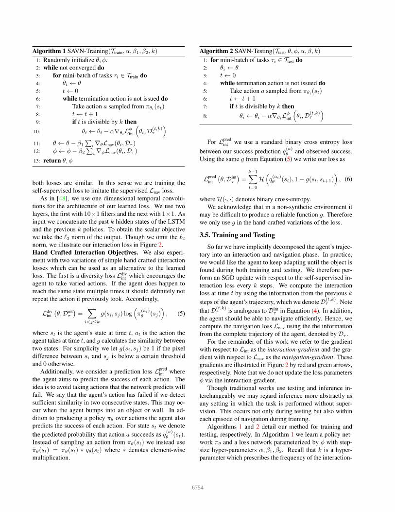
Algorithm 1 SAVN-Training(Ttrain, α, β1, β2, k)
1: Randomly initialize θ, φ.
2: while not converged do
3: for mini-batch of tasks τi ∈ Ttrain do
4: θi ← θ
5: t← 06: while termination action is not issued do
7: Take action a sampled from πθi(st)8: t← t+ 19: if t is divisible by k then
10: θi ← θi − α∇θiLφint
(
θi,D(t,k)τ
)
11: θ ← θ − β1
∑
i∇θLnav(θi,Dτ )12: φ← φ− β2
∑
i∇φLnav(θi,Dτ )
13: return θ, φ
both losses are similar. In this sense we are training the
self-supervised loss to imitate the supervised Lnav loss.
As in [48], we use one dimensional temporal convolu-
tions for the architecture of our learned loss. We use two
layers, the first with 10×1 filters and the next with 1×1. As
input we concatenate the past k hidden states of the LSTM
and the previous k policies. To obtain the scalar objective
we take the ℓ2 norm of the output. Though we omit the ℓ2norm, we illustrate our interaction loss in Figure 2.
Hand Crafted Interaction Objectives. We also experi-
ment with two variations of simple hand crafted interaction
losses which can be used as an alternative to the learned
loss. The first is a diversity loss Ldivint which encourages the
agent to take varied actions. If the agent does happen to
reach the same state multiple times it should definitely not
repeat the action it previously took. Accordingly,
Ldivint
(
θ,Dintτ
)
=∑
i<j≤k
g(si, sj) log(
π(ai)θ (sj)
)
, (5)
where st is the agent’s state at time t, at is the action the
agent takes at time t, and g calculates the similarity between
two states. For simplicity we let g(si, sj) be 1 if the pixel
difference between si and sj is below a certain threshold
and 0 otherwise.
Additionally, we consider a prediction loss Lpredint where
the agent aims to predict the success of each action. The
idea is to avoid taking actions that the network predicts will
fail. We say that the agent’s action has failed if we detect
sufficient similarity in two consecutive states. This may oc-
cur when the agent bumps into an object or wall. In ad-
dition to producing a policy πθ over actions the agent also
predicts the success of each action. For state st we denote
the predicted probability that action a succeeds as q(a)θ (st).
Instead of sampling an action from πθ(st) we instead use
πθ(st) = πθ(st) ∗ qθ(st) where ∗ denotes element-wise
multiplication.
Algorithm 2 SAVN-Testing(Ttest, θ, φ, α, β, k)
1: for mini-batch of tasks τi ∈ Ttest do
2: θi ← θ
3: t← 04: while termination action is not issued do
5: Take action a sampled from πθi(st)6: t← t+ 17: if t is divisible by k then
8: θi ← θi − α∇θiLφint
(
θi,D(t,k)τ
)
For Lpredint we use a standard binary cross entropy loss
between our success prediction q(a)θ and observed success.
Using the same g from Equation (5) we write our loss as
Lpredint
(
θ,Dintτ
)
=
k−1∑
t=0
H(
q(at)θ (st), 1− g(st, st+1)
)
, (6)
whereH(·, ·) denotes binary cross-entropy.
We acknowledge that in a non-synthetic environment it
may be difficult to produce a reliable function g. Therefore
we only use g in the hand-crafted variations of the loss.
3.5. Training and Testing
So far we have implicitly decomposed the agent’s trajec-
tory into an interaction and navigation phase. In practice,
we would like the agent to keep adapting until the object is
found during both training and testing. We therefore per-
form an SGD update with respect to the self-supervised in-
teraction loss every k steps. We compute the interaction
loss at time t by using the information from the previous k
steps of the agent’s trajectory, which we denoteD(t,k)τ . Note
that D(t,k)τ is analogous to Dint
τ in Equation (4). In addition,
the agent should be able to navigate efficiently. Hence, we
compute the navigation loss Lnav using the the information
from the complete trajectory of the agent, denoted by Dτ .
For the remainder of this work we refer to the gradient
with respect to Lint as the interaction-gradient and the gra-
dient with respect to Lnav as the navigation-gradient. These
gradients are illustrated in Figure 2 by red and green arrows,
respectively. Note that we do not update the loss parameters
φ via the interaction-gradient.
Though traditional works use testing and inference in-
terchangeably we may regard inference more abstractly as
any setting in which the task is performed without super-
vision. This occurs not only during testing but also within
each episode of navigation during training.
Algorithms 1 and 2 detail our method for training and
testing, respectively. In Algorithm 1 we learn a policy net-
work πθ and a loss network parameterized by φ with step-
size hyper-parameters α, β1, β2. Recall that k is a hyper-
parameter which prescribes the frequency of the interaction-
6754
! = #
! = $
! = %&
Bowl
Ou
r M
eth
od
No
n-A
da
pti
ve
Ba
seli
ne
Navigate to Television Navigate to Bowl Navigate to Lamp
! = #
! = $
! = %&
Bowl
! = #
! = $%$
! = &
TV
Lamp
! = #
! = $
! = %&
Lamp
! = #
! = $%
! = &&
(a) (b) (c)
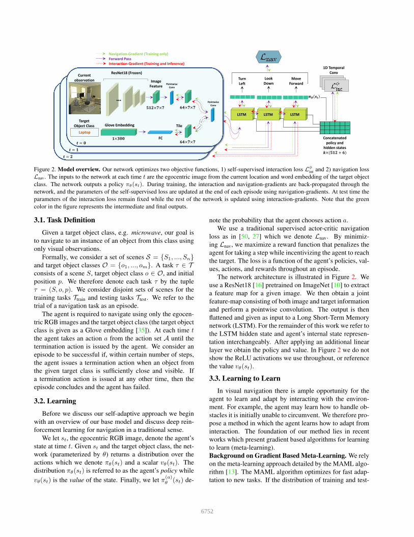
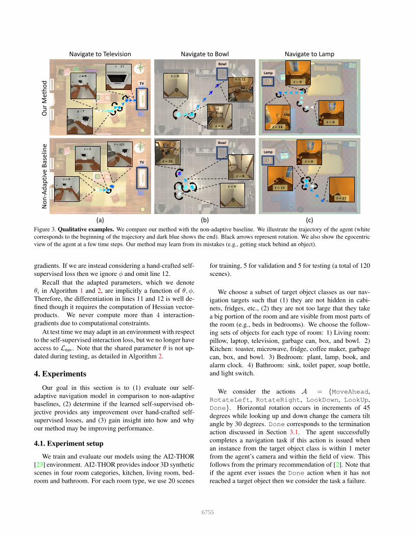
Figure 3. Qualitative examples. We compare our method with the non-adaptive baseline. We illustrate the trajectory of the agent (white
corresponds to the beginning of the trajectory and dark blue shows the end). Black arrows represent rotation. We also show the egocentric
view of the agent at a few time steps. Our method may learn from its mistakes (e.g., getting stuck behind an object).
gradients. If we are instead considering a hand-crafted self-
supervised loss then we ignore φ and omit line 12.
Recall that the adapted parameters, which we denote
θi in Algorithm 1 and 2, are implicitly a function of θ, φ.
Therefore, the differentiation in lines 11 and 12 is well de-
fined though it requires the computation of Hessian vector-
products. We never compute more than 4 interaction-
gradients due to computational constraints.
At test time we may adapt in an environment with respect
to the self-supervised interaction loss, but we no longer have
access to Lnav. Note that the shared parameter θ is not up-
dated during testing, as detailed in Algorithm 2.
4. Experiments
Our goal in this section is to (1) evaluate our self-
adaptive navigation model in comparison to non-adaptive
baselines, (2) determine if the learned self-supervised ob-
jective provides any improvement over hand-crafted self-
supervised losses, and (3) gain insight into how and why
our method may be improving performance.
4.1. Experiment setup
We train and evaluate our models using the AI2-THOR
[23] environment. AI2-THOR provides indoor 3D synthetic
scenes in four room categories, kitchen, living room, bed-
room and bathroom. For each room type, we use 20 scenes
for training, 5 for validation and 5 for testing (a total of 120
scenes).
We choose a subset of target object classes as our nav-
igation targets such that (1) they are not hidden in cabi-
nets, fridges, etc., (2) they are not too large that they take
a big portion of the room and are visible from most parts of
the room (e.g., beds in bedrooms). We choose the follow-
ing sets of objects for each type of room: 1) Living room:
pillow, laptop, television, garbage can, box, and bowl. 2)
Kitchen: toaster, microwave, fridge, coffee maker, garbage
can, box, and bowl. 3) Bedroom: plant, lamp, book, and
alarm clock. 4) Bathroom: sink, toilet paper, soap bottle,
and light switch.
We consider the actions A = {MoveAhead,
RotateLeft, RotateRight, LookDown, LookUp,
Done}. Horizontal rotation occurs in increments of 45
degrees while looking up and down change the camera tilt
angle by 30 degrees. Done corresponds to the termination
action discussed in Section 3.1. The agent successfully
completes a navigation task if this action is issued when
an instance from the target object class is within 1 meter
from the agent’s camera and within the field of view. This
follows from the primary recommendation of [2]. Note that
if the agent ever issues the Done action when it has not
reached a target object then we consider the task a failure.
6755
4.2. Implementation details
We train our method and baselines until the success rate
saturates on the validation set. We train one model across
all scene types with an equal number of episodes per type
using 12 asynchronous workers. For Lnav, we use a re-
ward of 5 for finding the object and -0.01 for taking a
step. For each scene we randomly sample an object from
the scene as a target along with a random initial position.
For our interaction-gradient updates we use SGD and for
our navigation-gradients we use Adam [22]. For step size
hyper-parameters (α, β1, β2 in Algorithm 1) we use 10−4
and for k we use 6. Recall that k is the hyper-parameter
which prescribes the frequency of interaction-gradients. We
experimented with a schedule for k but saw no significant
improvement in performance.
For evaluation we perform inference for 1000 different
episodes (250 for each scene type). The scene, initial state
of the agent and the target object are randomly chosen. All
models are evaluated using the same set. For each training
run we select the model that performs best on the validation
set in terms of success.
4.3. Evaluation metrics
We evaluate our method on unseen scenes using both
Success Rate and Success weighted by Path Length (SPL).
SPL was recently proposed by [2] and captures informa-
tion about navigation efficiency. Success is defined as1N
∑N
i=1 Si and SPL is defined as 1N
∑N
i=1 SiLi
max(Pi,Li),
where N is the number of episodes, Si is a binary indicator
of success in episode i, Pi denotes path length and Li is the
length of the optimal trajectory to any instance of the target
object class in that scene. We evaluate the performance of
our model both on all trajectories and trajectories where the
optimal path length is at least 5. We denote this by L ≥ 5(L refers to optimal trajectory length).
4.4. Baselines
We compare our models with the following baselines:
Random agent baseline. At each time step the agent ran-
domly samples an action using a uniform distribution.
Nearest neighbor (NN) baseline. At each time step we
select the most similar visual observation (in terms of Eu-
clidean distance between ResNet features) among scenes
in training set which contain an object of the class we are
searching for. We then take the action that is optimal in the
train scene when navigating to the same object class.
No adaptation (A3C) baseline. The architecture for the
baseline is the same as ours, however there is no interaction-
gradient and therefore no interaction loss. The training ob-
jective for this baseline is then minθ∑
τ∈TtrainLnav (θ,Dτ )
which is equivalent to setting α = 0 in Equation (4). This
baseline is trained using A3C [30].
All L ≥ 5SPL Success SPL Success
Random 3.64(0.6) 8.0(1.3) 0.1(0.1) 0.28(0.1)NN 6.09 7.90 1.38 1.66
No Adapt (A3C) 14.68(1.8) 33.04(3.5) 11.69(1.9) 21.44(3.0)Scene Priors [46] 15.47(1.1) 35.13(1.3) 11.37(1.6) 22.25(2.7)Ours - prediction 14.36(1.1) 38.06(2.9) 12.61(1.3) 26.41(2.4)Ours - diversity 15.12(1.5) 39.52(3.0) 13.38(1.4) 27.66(3.5)Ours - SAVN 16.15(0.5) 40.86(1.2) 13.91(0.5) 28.70(1.5)
Table 1. Quantitative results. We compare variations of our
method with random, nearest neighbor and non-adaptive base-
lines. We consider two evaluation metrics, Success Rate and SPL.
We provide results for all targets ‘All’ and a subset of targets whose
optimal trajectory length is greater than 5. We report the average
over 5 training runs with standard deviations shown in sub-scripted
parentheses.
4.5. Results
Table 1 summarizes the results of our approach and the
baselines. We consider three variations of our method,
which include SAVN (learned self-supervised loss) and the
hand-crafted prediction and diversity loss alternatives.
Our learned self-supervised loss outperforms all base-
lines by a large margin in terms of both success rate and
SPL metrics. Most notably, we observe about 8% abso-
lute improvement in success and 1.5 in SPL over the non-
adaptive (A3C) baseline. The self-supervised objective not
only learns to navigate more effectively but it also learns to
navigate efficiently.
The models trained with hand-crafted exploration losses
outperform our baselines by large margins in success, how-
ever, the SPL performance is not as impressive as with the
learned loss. We hypothesize that minimizing these hand-
crafted exploration losses are not as conducive to efficient
navigation.
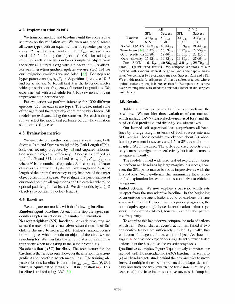
Failed actions. We now explore a behavior which sets
us apart from the non-adaptive baseline. In the beginning
of an episode the agent looks around or explores the free
space in front of it. However, as the episode progresses, the
non-adaptive agent might issue the termination action or get
stuck. Our method (SAVN), however, exhibits this pattern
less frequently.
To examine this behavior we compute the ratio of actions
which fail. Recall that an agent’s action has failed if two
consecutive frames are sufficiently similar. Typically, this
will occur if an agent collides with an object. As shown in
Figure 4, our method experiences significantly fewer failed
actions than the baseline as the episode progresses.
Qualitative examples. Figure 3 qualitatively compares our
method with the non-adaptive (A3C) baseline. In scenario
(a) our baseline gets stuck behind the box and tries to move
forward multiple times, while our method adapts dynami-
cally and finds the way towards the television. Similarly in
scenario (c), the baseline tries to move towards the lamp but
6756
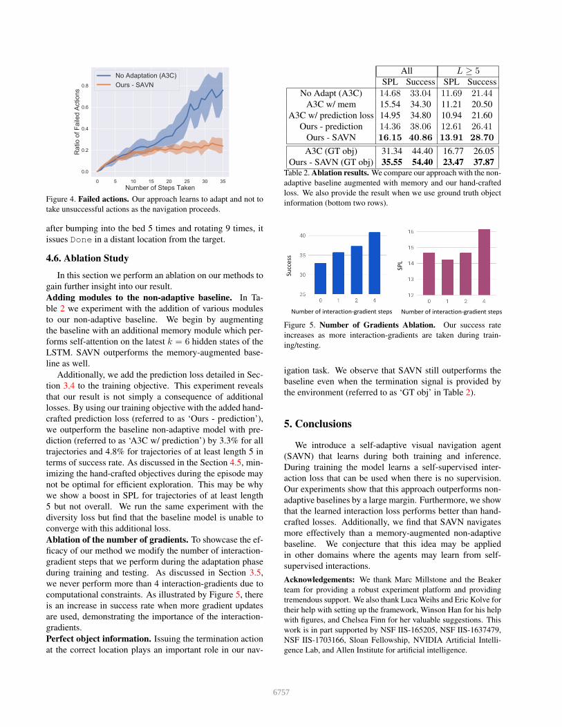
Figure 4. Failed actions. Our approach learns to adapt and not to
take unsuccessful actions as the navigation proceeds.
after bumping into the bed 5 times and rotating 9 times, it
issues Done in a distant location from the target.
4.6. Ablation Study
In this section we perform an ablation on our methods to
gain further insight into our result.
Adding modules to the non-adaptive baseline. In Ta-
ble 2 we experiment with the addition of various modules
to our non-adaptive baseline. We begin by augmenting
the baseline with an additional memory module which per-
forms self-attention on the latest k = 6 hidden states of the
LSTM. SAVN outperforms the memory-augmented base-
line as well.
Additionally, we add the prediction loss detailed in Sec-
tion 3.4 to the training objective. This experiment reveals
that our result is not simply a consequence of additional
losses. By using our training objective with the added hand-
crafted prediction loss (referred to as ‘Ours - prediction’),
we outperform the baseline non-adaptive model with pre-
diction (referred to as ‘A3C w/ prediction’) by 3.3% for all
trajectories and 4.8% for trajectories of at least length 5 in
terms of success rate. As discussed in the Section 4.5, min-
imizing the hand-crafted objectives during the episode may
not be optimal for efficient exploration. This may be why
we show a boost in SPL for trajectories of at least length
5 but not overall. We run the same experiment with the
diversity loss but find that the baseline model is unable to
converge with this additional loss.
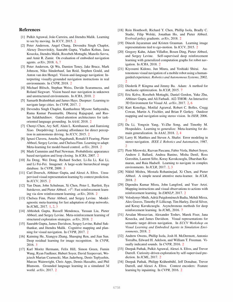
Ablation of the number of gradients. To showcase the ef-
ficacy of our method we modify the number of interaction-
gradient steps that we perform during the adaptation phase
during training and testing. As discussed in Section 3.5,
we never perform more than 4 interaction-gradients due to
computational constraints. As illustrated by Figure 5, there
is an increase in success rate when more gradient updates
are used, demonstrating the importance of the interaction-
gradients.
Perfect object information. Issuing the termination action
at the correct location plays an important role in our nav-
All L ≥ 5SPL Success SPL Success
No Adapt (A3C) 14.68 33.04 11.69 21.44A3C w/ mem 15.54 34.30 11.21 20.50
A3C w/ prediction loss 14.95 34.80 10.94 21.60
Ours - prediction 14.36 38.06 12.61 26.41Ours - SAVN 16.15 40.86 13.91 28.70
A3C (GT obj) 31.34 44.40 16.77 26.05
Ours - SAVN (GT obj) 35.55 54.40 23.47 37.87Table 2. Ablation results. We compare our approach with the non-
adaptive baseline augmented with memory and our hand-crafted
loss. We also provide the result when we use ground truth object
information (bottom two rows).
Success
Numberofinteraction-gradientsteps
SPL
Numberofinteraction-gradientsteps
Figure 5. Number of Gradients Ablation. Our success rate
increases as more interaction-gradients are taken during train-
ing/testing.
igation task. We observe that SAVN still outperforms the
baseline even when the termination signal is provided by
the environment (referred to as ‘GT obj’ in Table 2).
5. Conclusions
We introduce a self-adaptive visual navigation agent
(SAVN) that learns during both training and inference.
During training the model learns a self-supervised inter-
action loss that can be used when there is no supervision.
Our experiments show that this approach outperforms non-
adaptive baselines by a large margin. Furthermore, we show
that the learned interaction loss performs better than hand-
crafted losses. Additionally, we find that SAVN navigates
more effectively than a memory-augmented non-adaptive
baseline. We conjecture that this idea may be applied
in other domains where the agents may learn from self-
supervised interactions.
Acknowledgements: We thank Marc Millstone and the Beaker
team for providing a robust experiment platform and providing
tremendous support. We also thank Luca Weihs and Eric Kolve for
their help with setting up the framework, Winson Han for his help
with figures, and Chelsea Finn for her valuable suggestions. This
work is in part supported by NSF IIS-165205, NSF IIS-1637479,
NSF IIS-1703166, Sloan Fellowship, NVIDIA Artificial Intelli-
gence Lab, and Allen Institute for artificial intelligence.
6757
References
[1] Pulkit Agrawal, Joao Carreira, and Jitendra Malik. Learning
to see by moving. In ICCV, 2015. 2
[2] Peter Anderson, Angel Chang, Devendra Singh Chaplot,
Alexey Dosovitskiy, Saurabh Gupta, Vladlen Koltun, Jana
Kosecka, Jitendra Malik, Roozbeh Mottaghi, Manolis Savva,
and Amir R. Zamir. On evaluation of embodied navigation
agents. arXiv, 2018. 6, 7
[3] Peter Anderson, Qi Wu, Damien Teney, Jake Bruce, Mark
Johnson, Niko Sunderhauf, Ian Reid, Stephen Gould, and
Anton van den Hengel. Vision-and-language navigation: In-
terpreting visually-grounded navigation instructions in real
environments. In CVPR, 2018. 2
[4] Michael Blosch, Stephan Weiss, Davide Scaramuzza, and
Roland Siegwart. Vision based mav navigation in unknown
and unstructured environments. In ICRA, 2010. 2
[5] Samarth Brahmbhatt and James Hays. Deepnav: Learning to
navigate large cities. In CVPR, 2017. 2
[6] Devendra Singh Chaplot, Kanthashree Mysore Sathyendra,
Rama Kumar Pasumarthi, Dheeraj Rajagopal, and Rus-
lan Salakhutdinov. Gated-attention architectures for task-
oriented language grounding. In AAAI, 2018. 2
[7] Chenyi Chen, Ary Seff, Alain L. Kornhauser, and Jianxiong
Xiao. Deepdriving: Learning affordance for direct percep-
tion in autonomous driving. In ICCV, 2015. 2
[8] Ignasi Clavera, Anusha Nagabandi, Ronald S Fearing, Pieter
Abbeel, Sergey Levine, and Chelsea Finn. Learning to adapt:
Meta-learning for model-based control. arXiv, 2018. 2
[9] Mark Cummins and Paul Newman. Probabilistic appearance
based navigation and loop closing. In ICRA, 2007. 2
[10] Jia Deng, Wei Dong, Richard Socher, Li-Jia Li, Kai Li,
and Li Fei-Fei. Imagenet: A large-scale hierarchical image
database. In CVPR, 2009. 3
[11] Carl Doersch, Abhinav Gupta, and Alexei A. Efros. Unsu-
pervised visual representation learning by context prediction.
In ICCV, 2015. 2
[12] Yan Duan, John Schulman, Xi Chen, Peter L. Bartlett, Ilya
Sutskever, and Pieter Abbeel. rl2: Fast reinforcement learn-
ing via slow reinforcement learning. arXiv, 2016. 2
[13] Chelsea Finn, Pieter Abbeel, and Sergey Levine. Model-
agnostic meta-learning for fast adaptation of deep networks.
In ICML, 2017. 1, 2, 3
[14] Abhishek Gupta, Russell Mendonca, Yuxuan Liu, Pieter
Abbeel, and Sergey Levine. Meta-reinforcement learning of
structured exploration strategies. arXiv, 2018. 2
[15] Saurabh Gupta, James Davidson, Sergey Levine, Rahul Suk-
thankar, and Jitendra Malik. Cognitive mapping and plan-
ning for visual navigation. In CVPR, 2017. 2
[16] Kaiming He, Xiangyu Zhang, Shaoqing Ren, and Jian Sun.
Deep residual learning for image recognition. In CVPR,
2016. 3
[17] Karl Moritz Hermann, Felix Hill, Simon Green, Fumin
Wang, Ryan Faulkner, Hubert Soyer, David Szepesvari, Wo-
jciech Marian Czarnecki, Max Jaderberg, Denis Teplyashin,
Marcus Wainwright, Chris Apps, Demis Hassabis, and Phil
Blunsom. Grounded language learning in a simulated 3d
world. arXiv, 2017. 2
[18] Rein Houthooft, Richard Y. Chen, Phillip Isola, Bradly C.
Stadie, Filip Wolski, Jonathan Ho, and Pieter Abbeel.
Evolved policy gradients. arXiv, 2018. 2
[19] Dinesh Jayaraman and Kristen Grauman. Learning image
representations tied to ego-motion. In ICCV, 2015. 2
[20] Gregory Kahn, Adam Villaflor, Bosen Ding, Pieter Abbeel,
and Sergey Levine. Self-supervised deep reinforcement
learning with generalized computation graphs for robot nav-
igation. In ICRA, 2018. 2
[21] Kiyosumi Kidono, Jun Miura, and Yoshiaki Shirai. Au-
tonomous visual navigation of a mobile robot using a human-
guided experience. Robotics and Autonomous Systems, 2002.
2
[22] Diederik P. Kingma and Jimmy Ba. Adam: A method for
stochastic optimization. In ICLR, 2015. 7
[23] Eric Kolve, Roozbeh Mottaghi, Daniel Gordon, Yuke Zhu,
Abhinav Gupta, and Ali Farhadi. AI2-THOR: An Interactive
3D Environment for Visual AI. arXiv, 2017. 2, 6
[24] Kurt Konolige, Motilal Agrawal, Robert C. Bolles, Cregg
Cowan, Martin A. Fischler, and Brian P. Gerkey. Outdoor
mapping and navigation using stereo vision. In ISER, 2006.
2
[25] Da Li, Yongxin Yang, Yi-Zhe Song, and Timothy M.
Hospedales. Learning to generalize: Meta-learning for do-
main generalization. In AAAI, 2018. 2, 4
[26] Larry H. Matthies and Steven A. Shafer. Error modeling in
stereo navigation. IEEE J. Robotics and Automation, 1987.
2
[27] Piotr Mirowski, Razvan Pascanu, Fabio Viola, Hubert Soyer,
Andrew J. Ballard, Andrea Banino, Misha Denil, Ross
Goroshin, Laurent Sifre, Koray Kavukcuoglu, Dharshan Ku-
maran, and Raia Hadsell. Learning to navigate in complex
environments. In ICLR, 2017. 2, 3
[28] Nikhil Mishra, Mostafa Rohaninejad, Xi Chen, and Pieter
Abbeel. A simple neural attentive meta-learner. In ICLR,
2018. 2
[29] Dipendra Kumar Misra, John Langford, and Yoav Artzi.
Mapping instructions and visual observations to actions with
reinforcement learning. In EMNLP, 2017. 2
[30] Volodymyr Mnih, Adria Puigdomenech Badia, Mehdi Mirza,
Alex Graves, Timothy P. Lillicrap, Tim Harley, David Silver,
and Koray Kavukcuoglu. Asynchronous methods for deep
reinforcement learning. In ICML, 2016. 7
[31] Arsalan Mousavian, Alexander Toshev, Marek Fiser, Jana
Kosecka, and James Davidson. Visual representations for
semantic target driven navigation. In ECCV Workshop on
Visual Learning and Embodied Agents in Simulation Envi-
ronments, 2018. 2
[32] Andrew Owens, Phillip Isola, Josh H. McDermott, Antonio
Torralba, Edward H. Adelson, and William T. Freeman. Vi-
sually indicated sounds. In CVPR, 2016. 2
[33] Deepak Pathak, Pulkit Agrawal, Alexei A. Efros, and Trevor
Darrell. Curiosity-driven exploration by self-supervised pre-
diction. In ICML, 2017. 2
[34] Deepak Pathak, Philipp Krahenbuhl, Jeff Donahue, Trevor
Darrell, and Alexei A. Efros. Context encoders: Feature
learning by inpainting. In CVPR, 2016. 2
6758
[35] Jeffrey Pennington, Richard Socher, and Christopher D.
Manning. Glove: Global vectors for word representation.
In EMNLP, 2014. 3
[36] Lerrel Pinto, Dhiraj Gandhi, Yuanfeng Han, Yong-Lae Park,
and Abhinav Gupta. The curious robot: Learning visual rep-
resentations via physical interactions. In ECCV, 2016. 2
[37] Nikolay Savinov, Alexey Dosovitskiy, and Vladlen Koltun.
Semi-parametric topological memory for navigation. In
ICLR, 2018. 2
[38] Jurgen Schmidhuber, Jieyu Zhao, and Marco Wiering. Shift-
ing inductive bias with success-story algorithm, adaptive
levin search, and incremental self-improvement. Machine
Learning, 1997. 2
[39] Bradly C. Stadie, Sergey Levine, and Pieter Abbeel. Incen-
tivizing exploration in reinforcement learning with deep pre-
dictive models. arXiv, 2015. 2
[40] Sebastian Thrun. Learning metric-topological maps for in-
door mobile robot navigation. Artificial Intelligence, 1998.
2
[41] Sebastian Thrun and Lorien Pratt. Learning to Learn: Intro-
duction and Overview. 1998. 2
[42] Xiaolong Wang and Abhinav Gupta. Unsupervised learning
of visual representations using videos. In ICCV, 2015. 2
[43] Yuxin Wu and Yuandong Tian. Training agent for first-
person shooter game with actor-critic curriculum learning.
In ICLR, 2017. 2
[44] Yi Wu, Yuxin Wu, Aviv Tamar, Stuart J. Russell, Georgia
Gkioxari, and Yuandong Tian. Learning and planning with a
semantic model. arXiv, 2018. 2
[45] Tianbing Xu, Qiang Liu, Liang Zhao, and Jian Peng. Learn-
ing to explore with meta-policy gradient. In ICML, 2018.
2
[46] Wei Yang, Xiaolong Wang, Ali Farhadi, Abhinav Gupta, and
Roozbeh Mottaghi. Visual semantic navigation using scene
priors. In ICLR, 2019. 2, 7
[47] Haonan Yu, Haichao Zhang, and Wei Xu. Interactive
grounded language acquisition and generalization in a 2d
world. In ICLR, 2018. 2
[48] Tianhe Yu, Chelsea Finn, Annie Xie, Sudeep Dasari, Tian-
hao Zhang, Pieter Abbeel, and Sergey Levine. One-shot im-
itation from observing humans via domain-adaptive meta-
learning. In RSS, 2018. 2, 4, 5
[49] Richard Zhang, Phillip Isola, and Alexei A. Efros. Colorful
image colorization. In ECCV, 2016. 2
[50] Yuke Zhu, Roozbeh Mottaghi, Eric Kolve, Joseph J Lim, Ab-
hinav Gupta, Li Fei-Fei, and Ali Farhadi. Target-driven vi-
sual navigation in indoor scenes using deep reinforcement
learning. In ICRA, 2017. 2, 3
6759
Related Documents

![Adaptive Gradient-Based Meta-Learning Methods · Meta-learning, or learning-to-learn (LTL) [52], has recently re-emerged as an important direction for developing algorithms for multi-task](https://static.cupdf.com/doc/110x72/5f87539ff07709589b5cf0df/adaptive-gradient-based-meta-learning-methods-meta-learning-or-learning-to-learn.jpg)