Learning temporal Bayesian networks for power plant diagnosis

Learning Temporal Bayesian Networks for

Power Plant Diagnosis

Pablo Hernandez-Leal1, L. Enrique Sucar1, Jesus A. Gonzalez1, Eduardo F.Morales1, and Pablo H. Ibarguengoytia2

1 National Institute of Astrophysics, Optics and ElectronicsTonantzintla, Puebla, Mexico2 Electrical Research InstituteCuernavaca, Morelos, Mexico

Abstract. Diagnosis in industrial domains is a complex problem, be-cause it includes uncertainty management and temporal reasoning. Dy-namic Bayesian Networks (DBN) can deal with this type of problem.However, they usually lead to complex models. Temporal Nodes BayesianNetworks (TNBNs) are an alternative to DBNs for temporal reasoning,that result in much simpler and efficient models in certain domains. How-ever, methods for learning this type of models from data have not beendeveloped. In this paper, we propose a learning algorithm to obtain thestructure and temporal intervals for TNBNs from data. The method hasthree phases: (i) obtain an initial interval approximation, (ii) learn thenetwork structure based on the intervals, and (iii) refine the intervals foreach temporal node. The number of possible sets of intervals is obtainedfor each temporal node based on a clustering algorithm and the set ofintervals that maximizes the prediction accuracy is selected. We appliedthe algorithm to learn a TNBN for predicting errors in a combined cyclepower plant. The proposed algorithm obtains a simple model with highpredictive accuracy.

1 Introduction

Power plants and their effective operation are vital to the development of in-dustries, schools, and even for our houses, for this reason they maintain strictregulations and quality standards. However, problems may appear and whenthese happen, human operators have to take decisions relying mostly on theirexperience to determine the best recovery action with very limited help from thesystem. In order to provide useful information to the operator, different modelshave been developed that can deal with the industrial diagnosis. These modelsmust manage uncertainty because real world information is usually imprecise,incomplete, and with errors (noisy). Furthermore, they must manage temporalreasoning, since the timing of occurrence of the events is an important piece ofinformation.

Bayesian Networks [9] are an alternative to deal with uncertainty that hasproven to be successful in various domains. Nevertheless, these models cannot

deal with temporal information. An extension of BNs called Dynamic BayesianNetworks, can deal with temporal information. DBNs can be seen as multipleslices of a static BN over time, with links between adjacent slices. Nonetheless,these models can become quite complex, in particular, when only a few importantevents occur over time.

Temporal Nodes Bayesian Networks (TNBNs) [1] are another extension ofBayesian Networks. They belong to a class of temporal models known as EventBayesian Networks [5]. TNBNs were proposed to manage uncertainty and tem-poral reasoning. In a TNBN, each Temporal Node has intervals associated toit. Each node represents an event or state change of a variable. An arc betweentwo Temporal Nodes corresponds to a causal–temporal relation. One interestingproperty of this class of models, in contrast to Dynamic Bayesian Networks, isthat the temporal intervals can differ in number and size.

TNBNs had been used in diagnosis and prediction of temporal faults in asteam generator of a fossil power plant [1]. However, one problem that appearswhen using TNBNs is that no learning algorithm exists, so, the model has to beobtained from external sources (i.e., a domain expert). This can be a hard andprone to error task. In this paper, we propose a learning algorithm to obtain thestructure and the temporal intervals for TNBNs from data, and apply it to thediagnosis of a combined cycle power plant.

The learning algorithm consists of three phases. In the first phase, we ob-tain an approximation of the intervals. F this, we apply a clustering algorithm.T we convert these clusters into initial intervals. For the second phase, the BNstructure is obtained with a structure learning algorithm [2]. The last step is per-formed to refine the intervals for each Temporal Node. Our algorithm obtainsthe number of possible sets of intervals for each configuration of the parents byclustering the data based on a Gaussian mixture model. It then selects the setof intervals that maximizes the prediction accuracy. We applied the proposedmethod to fault diagnosis in a subsystem of a power plant. The data was ob-tained from a power plant simulator. The structure and intervals obtained bythe proposed algorithm are compared to a uniform discretization and k-meansclustering algorithm; the results show that our approach creates a simpler TNBNwith high predictive accuracy.

2 Related Work

Bayesian Networks (BN) have been applied to industrial diagnosis [6] However,static BNs are not suited to deal with temporal information. For this reasonDynamic Bayesian Networks [3] were created. In a DBN, a copy of a base modelis done for each time stage. These copies are linked via a transition network whichis usually connected through links only allowing connections between consecutivestages (Markov property). The problem is that DBNs can become very complex;and this is unnecessary when dealing with problems for which there are only afew changes for each variable in the model. Moreover, DBNs are not capable of

managing different levels of time granularity. They a fixed time interval betweenstages.

In TNBN, each variable represents an event or state change. S only oneor a few instances of each variable are required. Assuming there is one or afew changes of a variable state in the temporal range of interest, n copies ofthe model are needed, and no assumption about the Markovian nature of theprocess is done. TNBNs can deal with multiple granularity, because the numberand the size of the intervals for each node can be different.

There are several methods to learn BNs from data [8]. Unfortunately, thealgorithms used to learn BNs cannot deal with the problem of learning temporalintervals. S these cannot be applied directly to learn TNBNs. To the best ofour knowledge, there is only one previous work that attempts to learn a TNBN.Liu et al. [7] proposed a method to build a TNBN from a temporal probabilistic

database. The method obtains the structure from a set of temporal dependen-cies in a probabilistic temporal relational model (PTRM). In order to build theTNBN, they obtain a variable ordering that maximizes the set of conditional in-dependence relations implied by a dependency graph obtained from the PTRM.Based on this order, a directed acyclic graph corresponding to the implied in-dependence relations is obtained, which represents the structure of the TNBN.The previous work assumes a known probabilistic temporal–relational modelfrom the domain of interest, which is not always the case. Building this PTRMcould be as difficult as building a TNBN. In contrast, our approach constructsthe TNBN directly from data, which in many applications is readily available orcan be generated, for instance, using a simulator.

3 Temporal Nodes Bayesian Networks

A Temporal Nodes Bayesian Network (TNBN) [1, 5] is composed by a set ofTemporal Nodes (TNs). TNs are connected by edges. Each edge represents acausal-temporal relationship between TNs. There is at most one state changefor each variable (TN) in the temporal range of interest. The value taken by thevariable represents the interval in which the event occurs. Time is discretized ina finite number of intervals, allowing a different number and duration of inter-vals for each node (multiple granularity). Each interval defined for a child noderepresents the possible delays between the occurrence of one of its parent events(cause) and the corresponding child event (effect). Some Temporal Nodes do nothave temporal intervals. These correspond to Instantaneous Nodes. Formally:

Definition 1. A TNBN is defined as a pair B = (G,Θ). G is a Directed

Acyclic Graph, G = (V,E). G is composed of V, a set of Temporal and In-

stantaneous Nodes; E a set of edges between Nodes. The Θ component corre-

sponds to the set of parameters that quantifies the network. Θ contains the values

Θvi = P (vi|Pa(vi)) for each vi ∈ V; where Pa(vi) represents the set of parents

of vi in G.

Definition 2. A Temporal Node, vi, is defined by a set of states S, each state is

defined by an ordered pair S = (λ, τ), where λ is the value of a random variable

and τ = [a, b] is the interval associated, with initial value a and final value b, thatcorresponds to the time interval in which the state change occurs. In addition,

each Temporal Node contains an extra default state s = (’no change’, ∅), whichhas no interval associated. If a Node has no intervals defined for all its states

then it receives the name of Instantaneous Node.

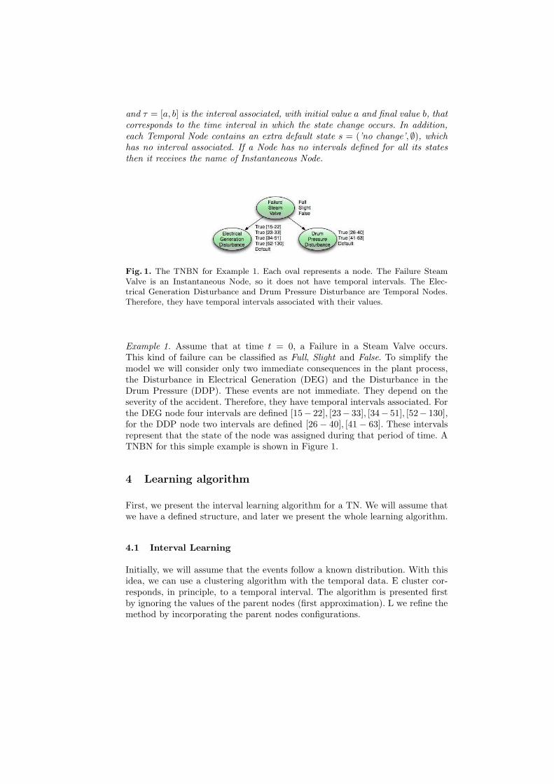
Fig. 1. The TNBN for Example 1. Each oval represents a node. The Failure SteamValve is an Instantaneous Node, so it does not have temporal intervals. The Elec-trical Generation Disturbance and Drum Pressure Disturbance are Temporal Nodes.Therefore, they have temporal intervals associated with their values.

Example 1. Assume that at time t = 0, a Failure in a Steam Valve occurs.This kind of failure can be classified as Full, Slight and False. To simplify themodel we will consider only two immediate consequences in the plant process,the Disturbance in Electrical Generation (DEG) and the Disturbance in theDrum Pressure (DDP). These events are not immediate. They depend on theseverity of the accident. Therefore, they have temporal intervals associated. Forthe DEG node four intervals are defined [15− 22], [23− 33], [34− 51], [52− 130],for the DDP node two intervals are defined [26 − 40], [41− 63]. These intervalsrepresent that the state of the node was assigned during that period of time. ATNBN for this simple example is shown in Figure 1.

4 Learning algorithm

First, we present the interval learning algorithm for a TN. We will assume thatwe have a defined structure, and later we present the whole learning algorithm.

4.1 Interval Learning

Initially, we will assume that the events follow a known distribution. With thisidea, we can use a clustering algorithm with the temporal data. E cluster cor-responds, in principle, to a temporal interval. The algorithm is presented firstby ignoring the values of the parent nodes (first approximation). L we refine themethod by incorporating the parent nodes configurations.

4.2 First approximation: independent variables

Our approach uses a Gaussian mixture model (GMM) to perform an approxi-mation of the data. Therefore, we can use the Expectation-Maximization (EM)algorithm [4]. EM works iteratively using two steps: (i) The E-step tries to guess

the parameters of the Gaussian distributions, (ii) the M-step updates the pa-rameters of the model based on the previous step. By applying EM, we obtain anumber of Gaussians (clusters), specified by their mean and variance. For now,assume that the number of temporal intervals (Gaussians), k, is given. For eachTN, we have a dataset of points over time, and these are clustered using GMM,to obtain k Gaussian distributions. Based on the parameters of each Gaussian,each temporal interval is initially defined by: [µ− σ, µ+ σ].

Now we will deal with the problem of finding the number of intervals. Theideal solution has to fulfill two conditions: (i) The number of intervals must besmall, in order to reduce the complexity of the network, and (ii) the intervalsshould yield good estimations when performing inference over the network. Basedon the above, our approach uses the EM algorithm with the parameter for thenumber of clusters in the range from 1 to ℓ, where ℓ is the highest value (for theexperiments in this paper we used ℓ = 3).

To select the best set of intervals, an evaluation is done over the network,which is an indirect measure of the quality of the intervals. In particular, weused the Relative Brier Score to measure the predictive accuracy of the network.The selected set of intervals for each TN, are those that maximize the RelativeBrier Score. The Brier Score is defined as BS =

∑n

i=1 (1− Pi)2, where Pi is

the marginal posterior probability of the correct value of each node given theevidence. The maximum brier score is BSmax =

∑n 1

2. The Relative Brier Score(RBS) is defined as: RBS (in %) = (1 − BS

BSmax

) × 100. This RBS is used toevaluate the TNBN instantiating a random subset of variables in the model,predicting the unseen variables, and obtaining the RBS for these predictions.

4.3 Second approximation: considering the network topology

Now we will construct a more precise approximation. For this, we use the con-figurations of the parent nodes. The number of configurations of each node i isqi =

∏Xt∈Pa(i) |st| (the product of the number of states of the parents nodes).

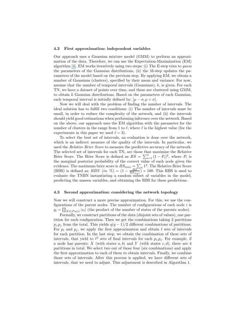
Formally, we construct partitions of the data (disjoint sets of values), one par-tition for each configuration. Then we get the combinations taking 2 partitionspi,pj from the total. This yields q(q − 1)/2 different combinations of partitions.For pi and pj, we apply the first approximation and obtain ℓ sets of intervalsfor each partition. In the last step, we obtain the combination of these sets ofintervals, that yield to ℓ2 sets of final intervals for each pi,pj . For example, ifa node has parents: X (with states a, b) and Y (with states c, d), there are 4partitions in total. We select two out of those four (six combinations) and applythe first approximation to each of them to obtain intervals. Finally, we combinethose sets of intervals. After this process is applied, we have different sets ofintervals, that we need to adjust. This adjustment is described in Algorithm 1.

Algorithm 1 Algorithm to adjust the intervals.

Require: Array of intervals setsEnsure: Array of intervals adjusted1: for Each set of intervals s do

2: sortIntervalsByStart(s)3: while Interval i is contained in Interval j do

4: tmp=AverageInterval(i,j)5: s.replaceInterval(i,j,tmp)6: end while

7: for k = 0 to number of intervals in set s-1 do

8: Interval[k].end=(Interval[k].end + Interval[k+1].start)/29: end for

10: end for

Algorithm 1 performs two nested loops. For each set of final intervals, we sortthe intervals by their starting point. T we check if there is an interval containedin another interval. While this is true, the algorithm obtains an average interval,taking the average of the start and end points of the intervals and replacing thesetwo intervals with the new one. Next, we refine the intervals to be continuousby taking the mean of two adjacent values.

As in the first approximation, the best set of intervals for each TN is selectedbased on the predictive accuracy in terms of the RBS. However, when a TN hasas parents other Temporal Nodes (an example of this situation is illustrated inFigure 3), the state of the parent nodes is not initially known. So, we cannotdirectly the second approximation. In order to solve this problem, the intervalsare selected sequentially in a top–down fashion according to the TNBN structure.That is, we first select the intervals for the nodes in the second level of thenetwork (the root nodes are instantaneous by definition in a TNBN [1]). Oncethese are defined, we know the values of the parents of the nodes in the 3rd level,so we can find their intervals; and so on, until the leaf nodes are reached.

4.4 Pruning

Taking the combinations and joining the intervals can become computationallytoo expensive. The number of sets of intervals per node is in O(q2ℓ2), for thisreason we used two pruning techniques for each TN to reduce the computationtime.

The first pruning technique discriminates the partitions that provide littleinformation to the model. For this, we count the number of instances in each

partition, and if it is greater than a value β = Number of instancesNumber of partitions×2

the con-

figuration is used, if not it is discarded. A second technique is applied when thefinal intervals for each combination are being obtained. If the final set of intervalscontains only one interval (no temporal information) or more than α (producinga complex network), the set of intervals is discarded. For our experiments, weused α = 4.

4.5 Structural Learning

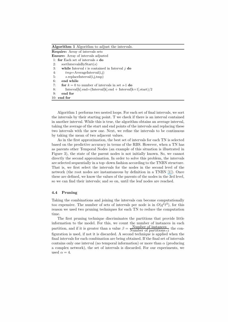
Algorithm 2 Algorithm to obtain the initial intervals

Require: Sorted Points Pi obtained by k-means algorithm, An array of continuousvalues data from Node n, min minimum value of data, max maximum value ofdata.

Ensure: Array of intervals for a Node n.1: Interval[0].start=min,Interval[0].end=average(point[0],point[1])2: for i=0 to size(Pi)-1 do

3: Interval[i+1].start=average(point[i],point[i+1]) ,4: Interval[i+1].end=average(point[i+1],point[i+2])5: end for

6: Interval[i].start=average(point[i],point[i+1]),Interval[i].end=max

Now we present the complete algorithm that learns the structure and theintervals of the TNBN. First we perform an initial discretization of the temporalvariables based on a clustering algorithm (k-means), the obtained clusters areconverted into intervals according to the process shown in Algorithm 2. With thisprocess, we obtain an initial approximation of the intervals for all the TemporalNodes, and we can perform a standard BN structural learning. We used the K2algorithm [2]. T algorithm has as a parameter an ordering of the nodes. Forlearning TNBN, we can exploit this parameter and define an order based ondomain information.

When a structure is obtained, we can apply the interval learning algorithmdescribed in Section 4.1. Moreover, this process of alternating interval learningand structure learning may be iterated until convergence. (With interval learningwe obtain intervals for each TN, and we can apply the K2 structure algorithm,then with the structure, we can perform the interval learning again.)

5 Application to Power Plant Diagnosis

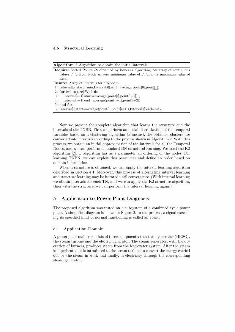
The proposed algorithm was tested on a subsystem of a combined cycle powerplant. A simplified diagram is shown in Figure 2. In the process, a signal exceed-ing its specified limit of normal functioning is called an event.

5.1 Application Domain

A power plant mainly consists of three equipments: the steam generator (HRSG),the steam turbine and the electric generator. The steam generator, with the op-eration of burners, produces steam from the feed-water system. After the steamis superheated, it is introduced to the steam turbine to convert the energy carriedout by the steam in work and finally, in electricity through the correspondingsteam generator.

Fig. 2. Schematic description of a power plant showing the feedwater and main steamsubsystems. Ffw refers to feedwater flow, Fms refers to main stream flow, dp refers todrum pressure, dl refers to drum level.

The HRSG consists of a huge boiler with an array of tubes, the drum andthe circulation pump. The feed-water flows through the tubes receiving the heatprovided by the gases from the gas turbine and the burners. Part of the watermass becomes steam and is separated from the water in a special tank calledthe drum. Here, water is stored to provide the boiler tubes with t appropriatevolume of liquid that will be evaporated and steam is stored to be sent to thesteam turbine.

From the drum, water is supplied to the rising water tubes called waterwalls by means of the water recirculation pump, where it will be evaporated,and water-steam mixture reaches the drum. From here, steam is supplied to thesteam turbine. The conversion of liquid water to steam is carried out at a specificsaturation condition of pressure and temperature. In this condition, water andsaturated steam are at the same temperature. This must be the stable condi-tion where the volume of water supply is commanded by the feed-water controlsystem. Furthermore, the valves that allow the steam supply to the turbine arecontrolled in order to manipulate the values of pressure in the drum. The levelof the drum is one of the most important variables in the generation process. Adecrease of the level may cause that not enough water is supplied to the risingtubes and the excess of heat and lack of cooling water may destroy the tubes.On the contrary, an excess of level in the drum may drag water as humidity inthe steam provided to the turbine and cause a severe damage in the blades. Inboth cases, a degradation of the performance of the generation cycle is observed.

Even with a very well calibrated instrument, controlling the level of the drumis one of the most complicated and uncertain processes of the whole generationsystem. This is because the mixture of steam and water makes very difficult thereading of the exact level of mass.

5.2 Experiments and Results

For obtaining the data used in the experiments, we used a full scale simulatorof the plant, then we simulate two failures randomly: failure in the Water Valveand failure in the Steam Valve. These types of failures are important because,they may cause disturbances in the generation capacity and the drum.

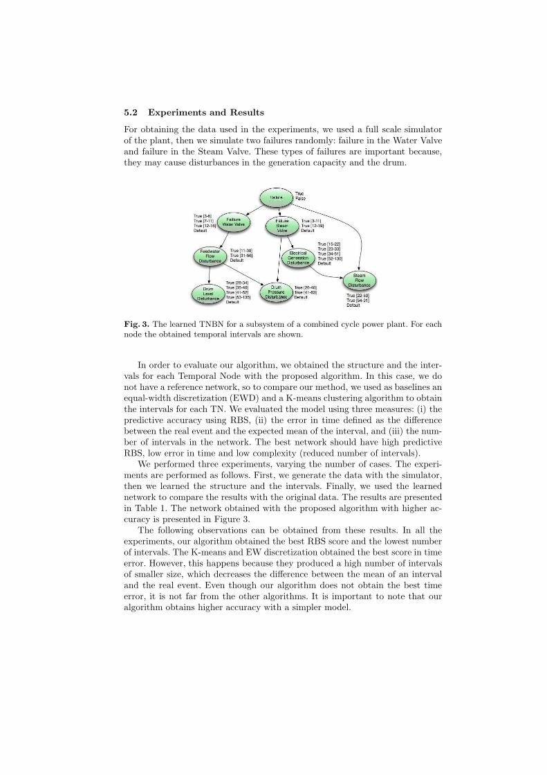
Fig. 3. The learned TNBN for a subsystem of a combined cycle power plant. For eachnode the obtained temporal intervals are shown.

In order to evaluate our algorithm, we obtained the structure and the inter-vals for each Temporal Node with the proposed algorithm. In this case, we donot have a reference network, so to compare our method, we used as baselines anequal-width discretization (EWD) and a K-means clustering algorithm to obtainthe intervals for each TN. We evaluated the model using three measures: (i) thepredictive accuracy using RBS, (ii) the error in time defined as the differencebetween the real event and the expected mean of the interval, and (iii) the num-ber of intervals in the network. The best network should have high predictiveRBS, low error in time and low complexity (reduced number of intervals).

We performed three experiments, varying the number of cases. The experi-ments are performed as follows. First, we generate the data with the simulator,then we learned the structure and the intervals. Finally, we used the learnednetwork to compare the results with the original data. The results are presentedin Table 1. The network obtained with the proposed algorithm with higher ac-curacy is presented in Figure 3.

The following observations can be obtained from these results. In all theexperiments, our algorithm obtained the best RBS score and the lowest numberof intervals. The K-means and EW discretization obtained the best score in timeerror. However, this happens because they produced a high number of intervalsof smaller size, which decreases the difference between the mean of an intervaland the real event. Even though our algorithm does not obtain the best timeerror, it is not far from the other algorithms. It is important to note that ouralgorithm obtains higher accuracy with a simpler model.

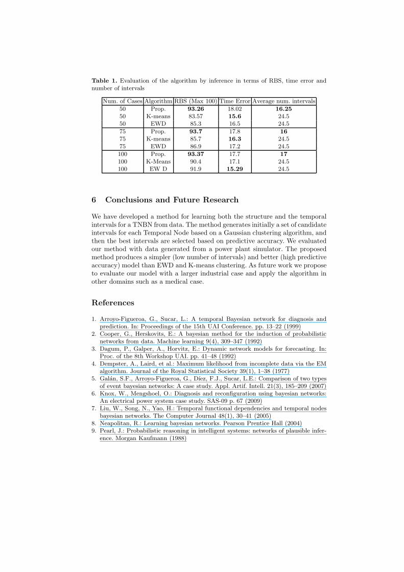
Table 1. Evaluation of the algorithm by inference in terms of RBS, time error andnumber of intervals

Num. of Cases Algorithm RBS (Max 100) Time Error Average num. intervals

50 Prop. 93.26 18.02 16.25

50 K-means 83.57 15.6 24.550 EWD 85.3 16.5 24.5

75 Prop. 93.7 17.8 16

75 K-means 85.7 16.3 24.575 EWD 86.9 17.2 24.5

100 Prop. 93.37 17.7 17

100 K-Means 90.4 17.1 24.5100 EW D 91.9 15.29 24.5

6 Conclusions and Future Research

We have developed a method for learning both the structure and the temporalintervals for a TNBN from data. The method generates initially a set of candidateintervals for each Temporal Node based on a Gaussian clustering algorithm, andthen the best intervals are selected based on predictive accuracy. We evaluatedour method with data generated from a power plant simulator. The proposedmethod produces a simpler (low number of intervals) and better (high predictiveaccuracy) model than EWD and K-means clustering. As future work we proposeto evaluate our model with a larger industrial case and apply the algorithm inother domains such as a medical case.

References

1. Arroyo-Figueroa, G., Sucar, L.: A temporal Bayesian network for diagnosis andprediction. In: Proceedings of the 15th UAI Conference. pp. 13–22 (1999)

2. Cooper, G., Herskovits, E.: A bayesian method for the induction of probabilisticnetworks from data. Machine learning 9(4), 309–347 (1992)

3. Dagum, P., Galper, A., Horvitz, E.: Dynamic network models for forecasting. In:Proc. of the 8th Workshop UAI. pp. 41–48 (1992)

4. Dempster, A., Laird, et al.: Maximum likelihood from incomplete data via the EMalgorithm. Journal of the Royal Statistical Society 39(1), 1–38 (1977)

5. Galan, S.F., Arroyo-Figueroa, G., Dıez, F.J., Sucar, L.E.: Comparison of two typesof event bayesian networks: A case study. Appl. Artif. Intell. 21(3), 185–209 (2007)

6. Knox, W., Mengshoel, O.: Diagnosis and reconfiguration using bayesian networks:An electrical power system case study. SAS-09 p. 67 (2009)

7. Liu, W., Song, N., Yao, H.: Temporal functional dependencies and temporal nodesbayesian networks. The Computer Journal 48(1), 30–41 (2005)

8. Neapolitan, R.: Learning bayesian networks. Pearson Prentice Hall (2004)9. Pearl, J.: Probabilistic reasoning in intelligent systems: networks of plausible infer-

ence. Morgan Kaufmann (1988)