Learning Signaling Network Structures with Sparsely Distributed Data

Learning signaling network structures with sparselydistributed data

Citation Sachs, Karen et al. “Learning Signaling Network Structures withSparsely Distributed Data.” Journal of Computational Biology16.2 (2010): 201-212. © 2009 Mary Ann Liebert, Inc.

As Published http://dx.doi.org/10.1089/cmb.2008.07TT

Publisher Mary Ann Liebert, Inc.

Version Final published version

Accessed Thu Sep 29 03:34:29 EDT 2011

Citable Link http://hdl.handle.net/1721.1/60319

Terms of Use Article is made available in accordance with the publisher's policyand may be subject to US copyright law. Please refer to thepublisher's site for terms of use.

Detailed Terms

JOURNAL OF COMPUTATIONAL BIOLOGY

Volume 16, Number 2, 2009

© Mary Ann Liebert, Inc.

Pp. 201–212

DOI: 10.1089/cmb.2008.07TT

Learning Signaling Network Structures

with Sparsely Distributed Data

KAREN SACHS,1 SOLOMON ITANI,2 JENNIFER CARLISLE,2 GARRY P. NOLAN,1

DANA PE’ER,4 and DOUGLAS A. LAUFFENBURGER3

ABSTRACT

Flow cytometric measurement of signaling protein abundances has proved particularly

useful for elucidation of signaling pathway structure. The single cell nature of the data

ensures a very large dataset size, providing a statistically robust dataset for structure

learning. Moreover, the approach is easily scaled to many conditions in high throughput.

However, the technology suffers from a dimensionality constraint: at the cutting edge,

only about 12 protein species can be measured per cell, far from sufficient for most

signaling pathways. Because the structure learning algorithm (in practice) requires that

all variables be measured together simultaneously, this restricts structure learning to the

number of variables that constitute the flow cytometer’s upper dimensionality limit. To

address this problem, we present here an algorithm that enables structure learning for

sparsely distributed data, allowing structure learning beyond the measurement technology’s

upper dimensionality limit for simultaneously measurable variables. The algorithm assesses

pairwise (or n-wise) dependencies, constructs “Markov neighborhoods” for each variable

based on these dependencies, measures each variable in the context of its neighborhood,

and performs structure learning using a constrained search.

Key words: Bayesian networks, flow cytometry, graphical models, proteomics, signaling path-

ways.

1. INTRODUCTION

SIGNALING PATHWAYS PRESENT THE CELL’S FIRST line of response to environmental factors. Learning

the structure of biomolecular pathways such as signaling pathways is an important task, leading to

greater understanding of pathway interactions, improved insight into misregulated (disease) states, and

increased ability to intervene towards therapeutic ends. We have previously demonstrated the ability to

1Department of Microbiology and Immunology, Baxter Laboratory in Genetic Pharmacology, Stanford University

School of Medicine, Stanford, California.2Department of Electrical Engineering and Computer Science, Massachusetts Institute of Technology, Cambridge,

Massachusetts.3Department of Biological Engineering, Massachusetts Institute of Technology, Cambridge, Massachusetts.4Biological Sciences, Columbia University, New York, New York.

201

202 SACHS ET AL.

elucidate signaling pathway structure from single cell flow cytometric measurements, using Bayesian

network structure learning (Sachs et al., 2005). Bayesian networks are probabilistic models that represent

statistical dependencies among variables of interest, in our case, biomolecules such as proteins. They can

be used to perform structure learning, the elucidation of influence connections among variables, which

can reveal the underlying structure of signaling pathways. While most measurements of signaling pathway

molecules consist of bulk analysis—measurements performed on lysates from a large number of cells—

flow cytometry enables measurement of signaling pathway molecules in individual cells, yielding large

datasets. However, the flow cytometer is restricted in the number of biomolecules it can profile per sample

(actually per cell). Due to limitations of the technology, at best, approximately 12 protein species can be

profiled simultaneously.

In juxtaposition to this technical constraint, signaling pathways may contain dozens, hundreds or even

thousands of relevant proteins, depending on the scope of the pathway under consideration. In light

of this, a dimensionality constraint of 12 constitutes a serious limitation. Furthermore, the majority of

research labs have a much more limited measurement capability, with a maximum measured set size of

approximately 4, rendering structure learning impractical. We address this limitation here, by proposing

the Markov Neighborhood algorithm, a novel algorithm which relies on overlapping measurements of

subsets of the variables of interest. This algorithm is motivated by the problem described above, stemming

from a technical constraint of flow cytometry. But it applies equally well in any situation in which the

measurement technology is limited in dimensionality (e.g., automated microscopy), resulting in sparsely

distributed data. The algorithm integrates measured subsets into one global model. We present results

applying this algorithm to the problem of learning an eleven variable pathway from flow cytometry data

with an upper measurement limit of four molecules per experiment.

2. BACKGROUND

Below, we present background useful for understanding the problem at hand and our proposed solution.

We describe flow cytometry, introduce Bayesian networks, and provide an overview of our algorithm.

2.1. Flow cytometry

In flow cytometry, molecules of interest are bound by antibodies attached to a fluorophore, labeling each

profiled signaling molecule with a different color. Cells thus stained pass in a thin stream of fluid through

the beam of a laser or series of lasers, and absorb light, causing them to fluoresce. The emitted light is

detected and recorded, providing a readout of fluorescence, and, therefore, of the relative abundance of

the detected molecules (Herzenberg and Sweet, 1976; Perfetto et al., 2004).

Profiling thousands of cells per minute, the flow cytometer quickly provides a large and statistically robust

dataset, suitable for structure learning of the underlying signaling pathway influence structure. Furthermore,

it is easily scaled to perform measurements on many conditions in a high throughput, 96-well format.

The flow cytometer, however, suffers from a dimensionality constraint. Because of crowding in the

emission spectrum of the fluorophores, it becomes difficult to cleanly measure the abundance of many

colors, limiting the number of total colors that can be used. The constraint on the number of colors depends

on various parameters (such as the number and wavelength of the the lasers with which the flow cytometer is

equipped), such that the actual constraint varies from facility to facility. Many flow cytometers can handle

approximately four colors. At the cutting edge (using four to five lasers), approximately 12 signaling

molecules can be profiled in each individual cell (Krutzik et al., 2004; Krutzik and Nolan, 2003; Perez

et al., 2004; Perez and Nolan, 2002, 2006).

2.2. Bayesian networks

Bayesian networks (Pearl, 1988), represent probabilistic dependence relationships among multiple inter-

acting components (in our case, activated signaling proteins), illustrating the effects of pathway components

upon each other in the form of an influence diagram—a graph (G), and a joint probability distribution. In

LEARNING SIGNALING NETWORK STRUCTURES 203

the graph, the nodes represent variables (the biomolecules) and the edges represent dependencies (or more

precisely, the lack of edges indicate a conditional independency) (Pearl, 1988). Each directed edge originates

at the parent variable and ends at the child. For each variable, a conditional probability distribution (CPD)

quantitatively describes the form and magnitude of its dependence on its parent(s).

Bayesian networks have been used extensively in biology, to model regulatory pathways in both the

genetic (Hartemink et al., 2001; Friedman et al., 2000; Friedman, 2004) and the signaling pathway domain

(Sachs et al., 2002; Sachs et al., 2005; Woolf et al., 2005). The structure learning task consists of searching

the space of possible structures to find the one that bests reflects probabilistic relationships in a biological

dataset. Under appropriate conditions (such as the availability of (perturbational) data) and assumptions,

a causal model interpretation can be applied, indicating that the parent of a variable in the learned graph

causally influences the variable’s quantity (directly or indirectly) (Pearl and Verma, 1991; Heckerman et al.,

1999). Within this framework, structure learning can be used to elucidate the structure of interactions in

regulatory pathways.

Simultaneous measurements. Dependencies such as correlations can be assessed with pairwise mea-

surements, and in fact it is reasonable to assume that variables are correlated with each of their parents.

Why then is it not possible to determine the pathway influence structure based on pairwise measurements?

Why the requirement for simultaneous measurements of the variables?

The answer is that Bayesian network models represent global, beyond pairwise relationships. This may

be, for instance, a complex interaction by which three parents regulate a child variable—one parent

may only exert its effect when the other two parents are present, an interaction that cannot be detected

with pairwise measurements. Alternatively, the dependence of two variables may diminish when a third

variable is considered (the third variable renders the first two conditionally independent), as seen for

instance in the structure A ! B ! C , in which, in spite of a path of influence from A to C , A and

C are conditionally independent given B . The Bayesian network can elucidate complex, global influence

relationships, but this ability comes at a price, requiring a large number of datapoints of simultaneously

measured variables.

Learning pathway structure with missing data. Learning pathway structure from measured subsets

can be seen as a missing data problem. For each datapoint, a subset of the measurements are available (the

subset that is measured) while the remaining variables are missing. In Bayesian networks, missing data

can be handled readily (Friedman, 1998); however, when a lot of the data is missing, these approaches will

not perform well. Since we are interested in scaling up the number of modeled variables by a substantial

amount, a different approach must be used.

2.3. Algorithm overview

In this paper, we describe a biologically motivated approach to scaling up the number of variables

that can be considered for structure learning. The algorithm starts with a set of preliminary experiments

which determine which subsets may be useful, such subsets are termed “Markov neighborhoods,” with

one such neighborhood defined for each variable (Fig. 1). The neighborhood for each variable is de-

termined based on statistical dependencies detected between it and other variables, in the preliminary

experiments. We call these Markov neighborhoods, as we expect them to roughly contain a variable’s

Markov blanket, which consists of its parents, children, and other co-parents of its children. Specifically,

their primary intended goal is to provide an accurate set of candidate parents for the variable. Next,

the neighborhood of each variable is profiled with flow cytometric measurements. The size of each

neighborhood is far smaller than the total number of variables, rendering it more suitable for simultaneous

measurement by flow cytometry. Finally, Bayesian network structure learning is performed, with the search

constrained to allow only parent sets that have been simultaneously measured along with the child variable

(Fig. 2).

Pruning neighborhoods exceeding maximum measurable size. What happens when a neighborhood

exceeds the maximally measurable set size? In this case, the neighborhood may be pruned if conditions

permit (Fig. 3). Consider variable X with neighborhood size exceeding the maximum permitted size m

(i.e., number of neighborhood members exceeds m � 1). When this occurs, pruning proceeds as follows:

X plus m � 1 of its neighborhood members are measured simultaneously. The subgraph including only

X and its measured neighborhood members is learned, and examined for conditional independencies. If

204 SACHS ET AL.

FIG. 1. A depiction of Markov neighborhoods for three variables. The figure shows the conceptual (unknown)

underlying set of all influence interactions. Variables circled in red are among those considered for structure learning.

An initial set of pairwise or n-wise experiments are performed. Based on those experiments, statistical dependence

is assessed between each variable pair or variable set. For each variable, a neighborhood is selected (depicted as

black circles), containing all variables with which it shares a high statistical dependence. Additionally, perturbation

parents—variables which demonstrate influence based on perturbation data, but which do not necessarily show strong

statistical dependence—may be added to the neighborhoods (depicted as black squares). These are considered ancestors

whose “path distance” may be so large as to diminish detectable statistical dependence. The neighborhood for each

variable contains its set of heuristically chosen candidate parents.

the subgraph reveals a conditional independence between X and any members of its neighborhood, then

the neighborhood may be pruned of the variable demonstrating this conditional independence with X ,

as long as the conditioning variable is present. For instance, if the subgraph Z ! Y ! X is found,

demonstrating that X and Z are conditionally independent given Y , then Z may be pruned from the

X’s neighborhood, as long as Y is retained. The next set of m variables can then be selected from the

pruned algorithm, iterating until the neighborhood has shrunk sufficiently, or until no more conditional

independencies can be found. In the latter case, the relationship between X and its parents may be

undiscoverable by the algorithm. Alternatively, to conserve resources and reduce the number of required

experiments, the neighborhood may be pruned heuristically, by selecting neighborhood members based

on the strength of statistical dependencies. This method has the obvious advantage of requiring fewer

experiments.

Minimizing the number of measurements. When all variables are simultaneously observable, the

number of necessary experiment is equal to the number of conditions employed. When overlapping subsets

must be used, as in this algorithm, the number of experiments grows, adding cost and complexity to the

LEARNING SIGNALING NETWORK STRUCTURES 205

FIG. 2. Overview of the Markov neighborhood algorithm. Using a set of preliminary pariwise or n-wise

measurements, a neighborhood is defined for each variable, which includes all variables demonstrating sufficiently

high correlation (note that any metric of statistical dependence may be employed), such that they may be considered

candidate parents. Next, experiments are performed in which each variable is measured with all members of its Markov

neighborhood. In some cases, neighborhoods may need to be pruned to fit the measurement constraints of the flow

cytometer (not shown; see Fig. 3). Each experiment measures a subset of the total set of variables. Finally, Bayesian

network structure learning is performed with a constrained search, in which {child, parent} sets may only be considered

if the child and all parents have been measured simultaneously.

FIG. 3. Neighborhood pruning. Shown is the first step in neighborhood pruning. Assuming a measurable set size

of four, target variable C is measured with three members of its neighborhood. A subgraph among these variables

is learned. If the structure returned demonstrates a conditional independence, the neighborhood may be pruned. For

instance, if the subgraph A ! B ! C is returned, A may be pruned from the neighborhood, as long as B is retained.

The procedure then iterates, selecting, for example, C along with B , D, and E . Pruning can continue until the

neighborhood size shrinks to four total variables, or until all possibilities for finding conditional independencies have

been exhausted. Alternatively, to conserve resources and reduce the number of required experiments, the neighborhood

may be pruned heuristically, by selecting the three top neighborhood members and pruning the remaining members.

206 SACHS ET AL.

data gathering process. In the extreme case, if all possible subsets were measured, for n variables and

subset size m, the number of experiments is . n

m/. In the example presented in this work, n D 11 and

m D 4, for a total of 330 experiments, a prohibitively large number. Constructing neighborhoods based on

a small set of preliminary experiments yields a dramatic reduction in the number of needed measurements,

enabling the use of this algorithm in real-life practical studies.

3. THE MARKOV NEIGHBORHOOD ALGORITHM

Below, we formally describe the algorithm, including motivation, justifications, and several optional

modifications. The specifics of implementations will depend on the simplicity of the domain as well as

the desired degree of resource investment, with the more involved options requiring a larger number of

experiments.

The main incentive for this algorithm is the recovery of the structure of large networks of proteins from

limited measurement sets. In parallel, the number of experiments should be kept to a minimum. In this

section, we present an algorithm for structure learning from small data sets. In addition, we present several

additional modifications of the algorithm that offer better accuracy in exchange for a higher amount of

experiments. Finally, we discuss the algorithm and study why we believe it might give good results in

general.

3.1. Algorithm description

The most basic form of the algorithm has three main steps: Determining the neighborhoods of variables,

running constrained BN learning on measurements of those neighborhoods, and pruning the resulting graph

for parasitical edges. A more detailed description is as follows:

Algorithm. Markov Neighbor Algorithm

0: Start with N variables (proteins) fx1; : : : ; xN g, a set of conditions C , and a limit on the number of variables measured in one

experiment de such that de > 2.

1: [Probing experiments] Collect data from experiments such that for every condition c and pair of variables (xi ; xj ), there is an

experiment measuring xi and xj at the same time under condition c.

2: Call subroutine ‘detect Neighborhoods’ to recover the Markov neighborhood N.xi / for each variable xi .

3: Call subroutine ‘Perturbation Parents’ and add resulting parents of xi to N.xi /.

4: If a certain neighborhood is larger than the number of variables that can be measured under one experiment (9 i W jN.xi /j > de):

5: Prune that neighborhood down to the admissible size by removing the variables with the weakest correlation, or using

subroutine ‘Neighborhood Conditional Independencies’.

6: Alternatively, a set of experiments each measuring xi with a different subgroup of variables from N.xi / can be run.

7: [Neighborhood experiments] Collect data from experiments such that for every condition c and variable xi , there is an experiment

measuring xi and N.xi / at the same time under condition c. Call the experiments available E1; : : : ; EM .

8: Use Bayesian Network learning algorithm with the search constrained to graphs where 8 xi , 9j W �.xi / 2 Ej . Call the resulting

graph G.

9: [Ranking Edge Confidence] Find the edges in G that incur the least decrease in the Bayesian cost function when deleted, and

remove them from G.

The BN step is a regular BN search that is done in a restricted space, since to score a certain child/parent

set in the BN algorithm, we need them to be measured together. Thus the search is restricted to graphs

whose child/parent sets are measured in at least one of the neighborhoods. Since we are considering

a smaller search space, it might appear that the quality of the results is strongly compromised. In the

following section, we show that this doesn’t have to be the case.

Detecting Neighborhoods and deciding on which variables to include in a certain neighborhood is at the

heart of the MN algorithm. It can be accomplished in a number of alternate ways. The most basic subroutine

determines the variables that are most “indicative” of each xi and adds them to xi ’s neighborhood. We

include a variable xj in xi ’s neighborhood if under any condition, there is a strong dependence between

xj and xi :

LEARNING SIGNALING NETWORK STRUCTURES 207

Subroutine. Detect Neighborhoods

0: Start with a collection of experiments such that for every condition c 2 C and pair of variables (xi ; xj ), there is an experiment

measuring xi and xj at the same time under condition c.

1: Discretize the variables xi into L levels.a

2: For each c 2 C , and pairs of variables xi and xj (i ¤ j ):

3: Consider the experiment measuring xi and xj under c and compute OP.Xi /, the empirical marginal of Xi .

4: For l 2 f1; : : : ; Lg,

5: Compute OP.Xi jXj D l/.

6: Next l .

7: Let Vc.xi ; xj / D maxl Œl1.OP.Xi /; OP.Xi jXj D l//�; where l1.:; :/ is the l1 distance function.

8: Next c.

9: Let V.xi ; xj / D maxc ŒVc.xi ; xj /�:

10: For i 2 f1; : : : ; N g

11: Apply k-means to the xthi row of V to determine the most strongly dependent nodes, and classify those as the “neighbors”

of xi ; N.xi /:

12: Next i .

It is important for the results that every variable is measured with all of its parents at the same time. Thus

when a certain neighborhood is too large to be measured at once, attempting to prune that neighborhood

down is essential. Since the goal is to keep the parents of the variable (xi ) in its neighborhood, variables that

are independent of xi when conditioned on (some of) xi’s parents can be removed from the neighborhood.

More advanced pruning can be done to distinguish parents from children, but this requires perturbations

on variables in the neighborhood in general.

This pruning requires additional experiments to be run, since it needs measurements of the variable with

different candidate parents. Once a variable is removed from the neighborhood, it does not have to be

included in further experiments in this step.

Subroutine. Neighborhood Conditional Independencies

0: For each xi :

1: Start with a Neighborhood N.xi / such that m � jN.xi /j > de�1.

2: For each de�1-tuple of variables x1j ; : : : ; x

de�1

j in N.xi /,

3: [Elimination experiments] Collect data containing xi and x1j ; : : : ; x

de�1

j .

4: Do BN learning, or conditional independence checks on the set xi , x1j ; : : : ; x

de�1

j .

5: If xkj ? xi jx

lj , remove xk

j from N.xi /: The conditioning can be applied to sets of parents too.

6: Next de�1-tuple.

7: Next i .

If the pruning fails to make the neighborhood size small enough, two approaches can be used. A hard

cutoff can be used to determine the neighborhood. For example, the variables with most effect on xi will

be included in N.xi /, or prior knowledge from the literature can be used to indicate which variables are

the most likely parents. On the other hand, several experiments measuring xi with different collections of

its parents might be included in the BN learning step. This would improve the results in general, but a

huge number of experiments might be needed to cover all possible combinations.

We finally turn to the subroutine of detecting parents from perturbations. The premise of this subroutine

is that a variable’s children are most likely to be the ones affected most by a perturbation on that

variable. Thus, this subroutine has a parameter DN , which is the number of descendants detected by

perturbations that we include as children of the perturbed variable. This parameter can be determined

by prior knowledge and the degree of confidence in the perturbations (the quality of the inhibitors, for

example).

aA discussion of discretization approaches can be found in Sachs (2006).

208 SACHS ET AL.

Subroutine. Perturbation Parents

0: Start with a collection of experiments such that for every condition c 2 C and pair of variables (xi ; xj ), there is an experiment

measuring xi and xj at the same time under condition c.

1: For each single intervention c where the perturbed variable was xi :

2: For each j 2 f1; : : : ; N g:

3: Compute OPn.Xj /, the empirical marginal of Xj under no interventions.

4: Compute OPni .Xj /, the empirical marginal of Xj under the single-intervention c.

5: Evaluate some distance d (the l1 norm or KL divergence) between OPn.Xj / and OPni .Xj /.

6: Next j .

7: Include xi in the neighborhood of the DN variables with the largest corresponding d ’s.

8: Next j .

A final intricacy of the perturbations parents is in the case where a perturbation on variable y affects

variable x substantially, but x and y are not correlated statistically. In this case, y can be added to the

neighborhood of x without taking the place of one of the variables already in the neighborhood. This can

be done as follows: an experiment can be run with y and N.x/ measured together (without x). From that

experiment, the empirical distribution of Y jN.x/ can be determined. From this, the experiment with x

and N.x/ can be augmented with y (by choosing y according to Y jN.x/. This allows larger effective

neighborhoods, which in turn produces better results in the BN learning step.

3.2. Algorithm discussion

In this subsection we turn to the study the validity of the output of the Markov Neighborhood Algorithm.

We argue that with reasonable neighborhood sizes and some careful study, even the optimal results

recovered by the BN algorithm with full data can be reached.

Let the optimal graph recovered from the BN study on full data be GBN , and the optimal graph recovered

by the MNA with neighborhood size n be GMNA.n/. First note that in the BN scoring, measuring each

child/parent set simultaneously is sufficient for scoring. This is because the Bayesian score is the product

of probabilities of child/parent sets. This implies that if every child/parent set is measured simultaneously

in the MNA, GBN can be scored (or more accurately, GBN is in the restricted search space).

Two additional facts have to be accounted for: the measurement of each child/parent set and the correct

scoring of graphs. The second issue arises because different child/parent sets might in general belong to

a different number of neighborhoods, and thus we might have a different number of measurements for

different child/parent sets. One has to be careful because the Bayesian score is sensitive to the number of

measurements. This problem can be easily solved if the number of measurements (per neighborhood) is

large and the priors on the subgraphs (of child/parent sets) are inversely proportional to the amount of data

measuring the subgraphs. Alternatively, one can make sure that they use the same number of measurements

while scoring every child/parent set.

The previous two points tell us that if we make sure that all child/parent sets in GBN are measured in

a certain neighborhood, then GMNA.n/ D GBN . This is what motivates our methodology for choosing the

neighborhoods; we assume that parents are highly correlated with their children, or that perturbations on

them affect their children most. It is obvious why these assumptions are natural, additionally, using condi-

tional independence to prune the neighborhoods allows highly correlated grandparents and grandchildren

to be picked out.

Thus under our assumptions, the Markov Neighborhood algorithm will produce results that are close

to the results from BN learning on full data. Some parasitical edges might be enforced because of the

restrictions on the search space, and the last step in the MNA attempts to clear those edges out, to further

improve the results.

4. RESULTS

In this section, we demonstrate the utility of our algorithm with an example in which we build an eleven

variable model, using subsets of size four. The data consists of measurements of signaling molecules

LEARNING SIGNALING NETWORK STRUCTURES 209

important in T-cell signaling, measured under several activation and inhibition conditions as described in

Sachs et al. (2005). The variables modeled are the signaling molecules PKC, PKA, Raf, Mek, Erk, Akt,

Plc , PIP2, PIP3, p38, and Jnk. For a full description of signaling molecules and employed conditions,

see Sachs et al. (2005). We have previously built the eleven variable model using the complete dataset. In

this study, we sample from the full dataset to create subsets with a maximum measurement size of four.

We take advantage of the full eleven color dataset to synthesize smaller data subsets, while still enabling

a comparison of the results to the “ground truth” model, as determined by the model resulting from the

full dataset.

Neighborhoods were assessed based on k-means clustering, using pairwise correlations as the dependence

metric. For this variable set and data, a clear bimodality was found, such that the resulting clusters were

convincingly legitimate, though they may be less clearcut in other domains. All neighborhoods found

contained no more than four members, rendering pruning unnecessary. In cases where a “perturbation

parent” lacked correlation with the target variable, its dataset was augmented with its value as described

above.

Model results. The resulting model perfectly recapitulated all model edges from the original full data

result. However, at the same confidence cutoff, it contained nine additional edges: Jnk ! p38, Mek ! Jnk,

Mek ! Plc , Raf ! Akt, PKC ! Erk, PKC ! PIP3, PKA ! Plc , Mek ! Akt, and Mek ! Plc .

Where do these additional edges come from? For a hint, we look at the results from the full data model.

Our results are reported as averaged models as described in Sachs et al. (2005), in which the confidence

of each edge is determined by the weighted average of all high scoring models containing that edge. In

the full data results, all nine of these edges appear, as lower confidence edges, specifically, these nine

appear if the confidence cutoff is reduced from the original 0.85 to 0.76. Do these edges reflect accurate

influence connections? In some cases they do, for instance, in the connection between Raf and Akt, an

edge that is missed in the original model, due to its low confidence value. In other cases, they appear to

reflect a correlation induced by a hidden coparent, as is likely the case in the edge between Jnk and p38,

two MAPK’s which may be influenced by the same MAPKK’s or other upstream molecules. Still others

require further investigation to determine their validity.

These edges did not make the confidence cutoff in the original model. Why did their confidence shift in

these results? The answer most likely lies in the constrained search space- in the original model, a number

of different edges may have helped to constrain the global model, explaining dependencies in the data

about equally well. Because different model results contained different ones of these more minor edges,

none of them sustained a high confidence level once the models were averaged. In this constrained search,

many of the minor edges were not present in the search space (they did not appear in any neighborhood),

greatly strengthening the minor edges that did remain.

This means that even at a very high confidence cutoff, our algorithm yields a dense graph (26 edges,

compared to the 17 edges present in the original model). While these additional edges may reflect legitimate

connections, it is crucial nevertheless to assess a relative confidence between them, particularly in the

densely connected signaling space, where the conclusion that variables are not connected, or are less

strongly connected is nearly as important as the detection of connectivity. In other words, a graph indicating

that (nearly) all variables are connected to all other variables is not as informative as one indicating a relative

ranking to emphasize stronger, higher confidence edges.

Ranking model edges. Because of the shift in confidence of model edges, we employ an additional

approach to rank the confidence of the 26 edges present at confidence above 0.85 (in fact they mostly

boasted a confidence of 0.99 or greater). We rank the edges based on the decrease in the model score when

an edge is removed. Based on this criteria, of the seven weakest edges, six are edges that are also below

the confidence cutoff in the original model. When these are removed, the model contains three edges that

did not make the cutoff in the original model, and misses one edge (PKC ! Mek) that was strong in the

original model but did not make the cutoff based on this ranking criteria. For simplicity, the unpruned

dense model with 26 edges is not shown. The model with edges pruned as just described is shown in

Figure 4.

Number of employed experiments. As stated earlier, one goal of our algorithm assumptions is to min-

imize the number of needed measurements, to enable practical applications of this algorithm. Preliminary

pairwise experiments, when performed in sets of 4, require just seven separate measurements per condition

to account for all pairs of the eleven variables. When applicable, neighborhoods containing each other were

210 SACHS ET AL.

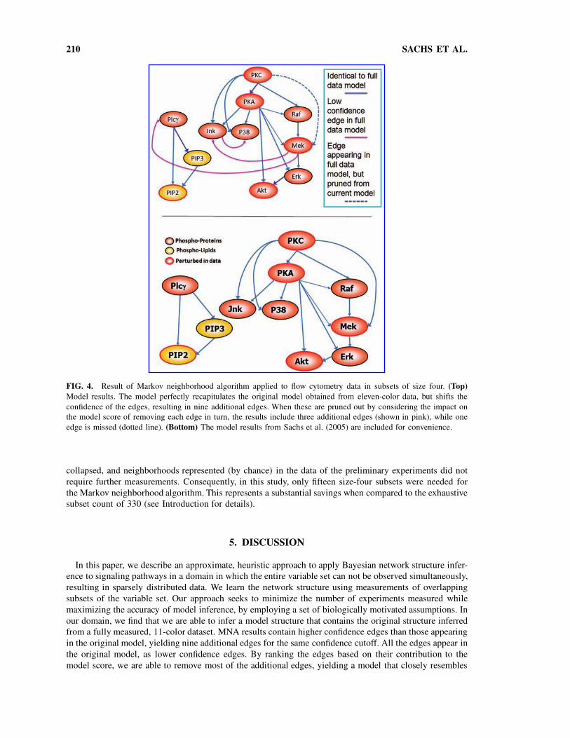
FIG. 4. Result of Markov neighborhood algorithm applied to flow cytometry data in subsets of size four. (Top)

Model results. The model perfectly recapitulates the original model obtained from eleven-color data, but shifts the

confidence of the edges, resulting in nine additional edges. When these are pruned out by considering the impact on

the model score of removing each edge in turn, the results include three additional edges (shown in pink), while one

edge is missed (dotted line). (Bottom) The model results from Sachs et al. (2005) are included for convenience.

collapsed, and neighborhoods represented (by chance) in the data of the preliminary experiments did not

require further measurements. Consequently, in this study, only fifteen size-four subsets were needed for

the Markov neighborhood algorithm. This represents a substantial savings when compared to the exhaustive

subset count of 330 (see Introduction for details).

5. DISCUSSION

In this paper, we describe an approximate, heuristic approach to apply Bayesian network structure infer-

ence to signaling pathways in a domain in which the entire variable set can not be observed simultaneously,

resulting in sparsely distributed data. We learn the network structure using measurements of overlapping

subsets of the variable set. Our approach seeks to minimize the number of experiments measured while

maximizing the accuracy of model inference, by employing a set of biologically motivated assumptions. In

our domain, we find that we are able to infer a model structure that contains the original structure inferred

from a fully measured, 11-color dataset. MNA results contain higher confidence edges than those appearing

in the original model, yielding nine additional edges for the same confidence cutoff. All the edges appear in

the original model, as lower confidence edges. By ranking the edges based on their contribution to the

model score, we are able to remove most of the additional edges, yielding a model that closely resembles

LEARNING SIGNALING NETWORK STRUCTURES 211

the original model. We note that the ability to rank edges is useful for prioritizing model results, even if

all edges map to causal connections.

One point for future work includes a more thorough theoretical treatment of the number of experiments

required, given in terms of the size of the Markov neighborhoods, the number of variables, n, and the

maximum measurable subset size, m. Or approach uses just 15 four-color experiments to accurately

reproduce the results of an 11-color experiment (albeit with a shift in confidence). However, these

results, particularly with regard to the number of measurements needed, are relevant for our particular

domain, with its set of variables and treatment conditions. A different domain may have a very different

correlation landscape, leading to very different requirement for experiments; furthermore, it may violate

our assumptions to varying degrees, yielding poorer results. Our work has an additional caveat: because

we simulate four-color data using an 11-color dataset, our data may be cleaner than data taken from actual

independent experiments, which may contain more variability. We do not believe this will be a major source

of variation, as the data is a moderately large sample drawn from the same distribution. Nevertheless, the

results must be interpreted with caution, as they are not conclusive regarding the number of experiments

needed or about the success of the modeling effort.

Although we present an example in which we scale up from a four-variable measurement capacity to

an 11-variable model, our intent is to enable a larger measurement capability to scale to larger models,

for instance, from 10 variables measured to models of 50–100. How would our approach differ for these

larger scale models? We can expect to need a larger number of experiments in order to initially cover each

pair of variables. On the other hand, the large scale models have the distinct advantage that, in contrast

to the smaller scale models, they are less likely to encounter a neighborhood larger than their maximum

measurable set size. This is because each signaling molecule has a finite, defined set of parents, so that

a measurement capability of �10 molecules can more easily accommodate each variable and its likely

parents than a four-color measurement capability. This fact also constrains the number of experiments that

are necessary, because the combinatorial step of measuring subsets of size m from large neighborhoods

is likely to be unnecessary. Although the details in terms of the number of experiments needed, and

the success of the results will depend on various factors (prominently, the correlation landscape of the

domain, and the particular dependencies among the variables, respectively), we anticipate that larger scale

models will prove more amenable to this approach than smaller models. This work proffers an approach

for approximate model inference in a pathway with a number of molecules exceeding our measurement

capabilities. Although our results are specific to just one particular variable set, they nonetheless indicate

the possibility that this approach is both feasible (in terms of the number of experiments required) and

effective (in terms of the modeling results). It is our hope that this method can be used to infer increasingly

large signaling pathway models. Particularly as measurement capabilities improve (for a cutting edge

multivariate, single cell approach with high dimensionality, Tanner et al. [2007]), it may be possible to

build highly integrated models involving numerous canonical pathways, in order to discover points of cross

talk, enrich our knowledge of various pathways, and enable a truly systems approach even in relatively

uncharted domains.

ACKNOWLEDGMENTS

We thank David Gifford for helpful discussions.

We gratefully acknowledge funding from the Leukemia and Lymphoma Society (postdoctoral fellowship

to K.S.), the NIH (grant AI06584 to D.A.L. and G.P.N., and grant GM68762 to D.A.L.), the Burroughs

Wellcome Fund (grant to D.P.), and the NIH (grants N01-HV-28183, U19 AI057229, 2P01 AI36535, U19

AI062623, R01-AI065824, 1P50 CA114747, 2P01 CA034233-22A1, and HHSN272200700038C, NCI

grant U54 RFA-CA-05-024 and LLS grant 7017-6 to G.P.N.).

DISCLOSURE STATEMENT

No competing financial interests exist.

212 SACHS ET AL.

REFERENCES

Friedman, N. 1998. The Bayesian structural EM algorithm. Proc. 14th Annu. Conf. Uncertainty AI, pgs. 129–138.

Friedman, N. 2004. Inferring cellular networks using probabilistic graphical models. Science 303:799–805.

Friedman, N., Linial, M., Nachman, I., et al. 2000. Using Bayesian networks to analyze expression data. J. Comput.

Biol. 7, 3–4.

Hartemink, A.J., Gifford, D.K., Jaakkola, T.S., et al. 2001. Using graphical models and genomic expression data to

statistically validate models of genetic regulatory networks. Pac. Symp. Biocomput. 422–433.

Heckerman, D., Meek, C., and Cooper, G.F. 1999. Computation, Causation, and Discovery, Glymour, C., and Cooper,

G.F., eds., MIT Press, Cambridge, MA.

Herzenberg, L.A., and Sweet, R.G. 1976. Fluorescence-activated cell sorting. Sci. Am. 234, 108–117.

Krutzik, P.O., Irish, J.M., Nolan, G.P., et al. 2004. Analysis of protein phosphorylation and cellular signaling events

by flow cytometry: techniques and clinical applications. Clin. Immunol. 110, 206–221.

Krutzik, P.O., and Nolan, G.P. 2003. Intracellular phospho-protein staining techniques for flow cytometry: monitoring

single cell signaling events. Cytometry A 55, 61–70.

Pearl, J. 1988. Probabilistic Reasoning in Intelligent Systems: Networks of Plausible Inference. Morgan Kauffman

Publishers, San Mateo, CA.

Pearl, J., and Verma, T.S. 1991. KR-91: Principles of knowledge representation and reasoning: Proc 2nd Intl Conf.,

Morgan Kaufmann, pgs. 441–452.

Perez, O.D., Krutzik, P.O., and Nolan, G.P. 2004. Flow cytometric analysis of kinase signaling cascades. Methods Mol.

Biol. 263, 67–94.

Perez, O.D., and Nolan, G.P. 2002. Simultaneous measurement of multiple active kinase states using polychromatic

flow cytometry. Nat. Biotechnol. 20, 155–162.

Perez, O.D., and Nolan, G.P. 2006. Phospho-proteomic immune analysis by flow cytometry: from mechanism to

translational medicine at the single-cell level. Immunol. Rev. 210, 208–228.

Perfetto, A., Chattopadhyay, P., and Roederer, M. 2004. Seventeen-colour flow cytometry: unravelling the immune

system. Nat. Rev. Immunol. 4, 648–655.

Sachs, K. 2006. Bayesian network models of biological signaling pathways [Ph.D. dissertation]. Massachussetts Institute

of Technology, Cambridge, MA.

Sachs, K., Gifford, D., Jakkola, T., et al. 2002. Bayesian network approach to cell signaling pathway modeling. Sci.

STKE, 148/38–42.

Sachs, K., Perez, O., Pe’er, D., et al. 2005. Causal protein-signaling networks derived from multiparameter single-cell

data. Science 308, 523–529.

Tanner, S.D., Ornatsky, O., Bandura, D.R., et al. 2007. Multiplex bio-assay with inductively coupled plasma mass

spectrometry: towards a massively multivariate single-cell technology. Spectrochim. Acta B: Atomic Spectrosc. 62,

188–195.

Woolf, P.J., Prudhomme, W., Daheron, L., et al. 2005. Bayesian analysis of signaling networks governing embryonic

stem cell fate decisions. Bioinformatics 21, 741–753.

Address reprint requests to:

Dr. Douglas A. Lauffenburger

Department of Biological Engineering

Massachusetts Institute of Technology

77 Massachusetts Avenue, 16-343

Cambridge, MA 02139

E-mail: [email protected]