Learning Saliency by MRF and Differential Threshold Learning Saliency by MRF and... · Learning Saliency by MRF and Differential Threshold Guokang Zhu, Qi Wang, Yuan Yuan, Senior

2032 IEEE TRANSACTIONS ON CYBERNETICS, VOL. 43, NO. 6, DECEMBER 2013

Learning Saliency by MRF andDifferential Threshold

Guokang Zhu, Qi Wang, Yuan Yuan, Senior Member, IEEE, and Pingkun Yan, Senior Member, IEEE

Abstract—Saliency detection has been an attractive topic inrecent years. The reliable detection of saliency can help a lot ofuseful processing without prior knowledge about the scene, suchas content-aware image compression, segmentation, etc. Althoughmany efforts have been spent in this subject, the feature expres-sion and model construction are far from perfect. The obtainedsaliency maps are therefore not satisfying enough. In order toovercome these challenges, this paper presents a new psychologicvisual feature based on differential threshold and applies it in asupervised Markov-random-field framework. Experiments on twopublic data sets and an image retargeting application demonstratethe effectiveness, robustness, and practicability of the proposedmethod.

Index Terms—Computer vision, differential threshold, machinelearning, Markov random field (MRF), saliency detection, visualattention.

I. INTRODUCTION

THE HUMAN visual system is remarkably effective atfinding particular objects from a scene. For instance,

when looking at images in the first row of Fig. 1, people areusually attracted by some specific objects within them (i.e.,strawberries, a leaf, a flag, a person, and a flower, respectively).This ability of the human visual system to identify the salientregions in the visual field can enable one to “withdraw fromsome things in order to deal effectively with others” [1], [2],i.e., allocate the limited perceptual processing resources in anefficient way. It is believed that visual processing involves twostages: a preattentive stage that processes all the informationavailable in parallel and, then, an attentive stage, in which thepartial information inside of the attentional spotlight is gluedtogether in serial for further processing [3]–[5]. In this paper,the preattentive functionality of the human visual system isimitated by a computer vision technique—saliency detection.

Manuscript received February 24, 2012; revised July 20, 2012 andDecember 3, 2012; accepted December 28, 2012. Date of publicationFebruary 21, 2013; date of current version November 18, 2013. This workwas supported in part by the National Basic Research Program of China(973 Program) under Grant 2011CB707104, by the National Natural ScienceFoundation of China under Grants 61172142, 61172143, 61105012, 61125106,and 91120302, by the Natural Science Foundation Research Project of ShaanxiProvince under Grant 2012JM8024, and by the 50th China Postdoctoral ScienceFoundation under Grant 2011M501487. This paper was recommended byEditor F. Hoffmann.

The authors are with the Center for OPTical IMagery Analysis and Learn-ing (OPTIMAL), State Key Laboratory of Transient Optics and Photonics,Xi’an Institute of Optics and Precision Mechanics, Chinese Academy ofSciences, Xi’an 710119, Shaanxi, P. R. China (e-mail: [email protected];[email protected]; [email protected]; [email protected]).

Color versions of one or more of the figures in this paper are available onlineat http://ieeexplore.ieee.org.

Digital Object Identifier 10.1109/TSMCB.2013.2238927

Saliency detection aims at providing the computational iden-tification of scene elements that are notable to human observers.The detected result is presented as a grayscale image. Thelighter the pixel is, the more salient it might be. Typical ex-amples of saliency detection results are demonstrated in Fig. 1.Implementing the functionality of human visual attention bymeans of saliency detection is considered to be an importantcomponent in computer vision because of a wide range of appli-cations, such as adaptive content delivery [6], video summariza-tion [7], image quality assessment [8], [9], content-aware imagecompression and scaling [10]–[12], image segmentation [13],[14], object detection [2], and object recognition [15]–[17].However, computer vision methods are still far from satisfyingcompared with biological systems. Therefore, researchers havenever stopped making efforts to provide a more effective andefficient method for automatic saliency detection.

A. Related Work

Classical saliency detection methods choose to employ a“low-level” approach to calculate contrasts of image regionswith respect to their surroundings, by selecting one or morelow-level features such as color, intensity, and orientation [18].The produced saliency results are topographically arrangedmaps, which integrate the normalized information from oneor more feature maps to represent the visual saliency of aspecific scene. According to the techniques that they used,these methods can broadly be categorized into three groups:biologically inspired, fully computational, and a combinationof them.

Biologically inspired methods are based on the imitation ofthe selective mechanism of the human visual system. Itti et al.[19] introduce a groundbreaking saliency model, which is in-spired by the biologically plausible architecture of the humanvisual system proposed by Koch and Ullman [21]. They firstextract multiscale features from three complementary channelsusing a difference of Gaussian (DoG) approach. Then, theacross-scale combination and normalization are employed tofuse the obtained features to an integrated saliency map. Basedon this work, Walther et al. [22] propose to recognize salient ob-jects in images by combining the saliency detection method of[19] with a hierarchical recognition model, while Frintrop et al.[23] capture saliency by computing center-surround differencesthrough square filters and employ integral images to speed upthe computation process. Recently, Garcia-Diaz et al. [24], [25]propose to take into account the perception role of nonclassicalreceptive fields. They start from the multiscale decompositionon the features of color and local orientation and use the

2168-2267 © 2013 IEEE

ZHU et al.: LEARNING SALIENCY BY MRF AND DIFFERENTIAL THRESHOLD 2033

Fig. 1. Saliency detection. From top to bottom, each row respectively represents the original images, the ground truths, and the saliency maps calculated by IT[19], HC [20], and the proposed method.

statistical distance between each feature and the center of thedistribution to produce the saliency map.

Different from biologically inspired methods, the fully com-putational methods calculate saliency maps directly by contrastanalysis [18]. For example, Achanta et al. [26] evaluate saliencyas the Euclidean distance between the average feature vectorsof the inner subregion of a sliding window and its neighborhoodregion. Later, in order to preserve the boundaries of salientobjects in the saliency map, Achanta et al. [18] present afrequency-tuned algorithm, which can retain more frequencycontent from the examined image than previous techniques.Gao et al. [27]–[29] model saliency detection as a classificationproblem. They measure the saliency value of a location as theKullback–Leibler divergence between the histogram of a seriesof DoG and Gabor filter responses at the point and its surround-ing region. Seo and Milanfar [30] propose to use local steeringkernels (LSKs) as features, which measure saliency in terms ofthe amount of gradient contrast between the examined locationand its surrounding region. Differently, Hou and Zhang [31]present a spectral residual method independent of low-levelimage features and prior knowledge. They start from a thoroughstatistics and experimental analysis of the log Fourier spectrumof natural images. Then, they propose to detect saliency bycalculating the contrast between the original and the locallyaveraged log Fourier spectrum of the examined image.

More recently, Rahtu et al. [32] propose a saliency measurebased on a Bayesian framework, which calculates the localcontrast of a set of low-level features in a sliding window.Goferman et al. [33] propose a context-aware saliency model,which aims at extracting an image subregion representing thescene and is based on the contrast between each image patchand the corresponding k most similar patches in the image. Liuet al. [34], [35] formulate the problem of saliency detection asan image segmentation task. In their method, novel featuressuch as center-surround histogram, multiscale contrast, and

color spatial distribution are employed to extract the promi-nent regions through conditional random field (CRF) learning.Cheng et al. [20] propose a regional saliency extraction methodsimultaneously evaluating the global contrast and spatial coher-ence. Wang et al. [36] define saliency as an anomaly relative to agiven context and detect salient regions in the image associatedwith a large dictionary of images through k-nearest-neighborretrieval.

The third category of methods is partly inspired by biologicalmodels and partly dependent on the techniques of fully compu-tational methods. For instance, Harel et al. [37] design a graph-based method, which first forms activation maps by using somecertain features (e.g., by default, color, intensity, and orientationmaps are computed) and then combines them in a mannerthat highlights conspicuity. Bruce and Tsotsos [38] describe abiologically plausible model of saliency detection based on themaximum information sampled from a scene and calculate theprobability density function based on a Gaussian kernel densityestimate in a neural circuit. Zhang et al. [39] provide a Bayesianframework for the saliency task. They consider saliency as theprobability of a target to be outstanding based on the analysisof Shannon’s self-information and mutual information. Otherthan these, Judd et al. [40] train a saliency detection model bysupport vector machine (SVM), which utilizes multilevel imagefeatures to tackle the eye-tracking data.

B. Limitations of Existing Methods

Although various methods for saliency detection have beenpresented in the past few years and a laudable performancefor human attentional spotlight prediction has been achieved insome circumstances, there are still several limitations for thesemethods.

The first limitation is the integration model. Although thereare large number of cues, such as color, texture, shape, depth,


Fig. 2. Summary of the proposed method. The salient object detection problem is modeled by an MRF, where a group of biologically inspired salient features isincorporated in the detection procedure through MRF learning.

shadow, and motion, which have been considered as influen-tial factors on visual attention in existing works, most of themainstream methods [18], [20], [30], [32], [39], [41] integratethem only based on direct contrast calculation, which is not ableto include priors. However, the ability to incorporate the priorinformation is important in many computer vision tasks [42].

Recently, learning-based methods have become very popularand seem to be generating promising results. However, thereare still remaining problems. For example, Judd et al. [40]employ an SVM classifier for saliency detection. The train-ing set employed in their work is composed of images withground-truth fixation points instead of regions. Sometimes, afew detected fixation points are adequate for further applica-tions. However, in most cases, the desired exports are salientregions.

The second limitation is the feature description. Manydescriptions of the saliency features [30], [32], [36], [43], [44]based on the aforementioned cues are only applicable to scene-specific database or limited by the strict conditions of use. Forexample, Seo and Milanfar [30] propose to use LSK as thesaliency feature descriptor based on the covariance matriceswithin the local windows. It is obvious that this definitionwill highlight regions with higher local complexity. However,saliency cannot always be equated with local complexity. Forexample, Fig. 1 shows that the much less complex regionscontaining the flag or the flower appear to be significantly moresalient. Wang et al. [36] describe saliency feature based onsearching through the enormous online image database. Theirmethod therefore greatly limits its promotion potential by theharsh conditions in practice.

In fact, there are many proverbial principles of the humanvision system, which can play a significant role in breakingthrough the bottleneck of constructing the more effective andcompact feature descriptions. Nevertheless, there is no sub-stantial progress in regard to ingeniously introducing theseprinciples into computer vision.

C. Overview of the Proposed Method

The presented method, named differential threshold andMarkov random field (MRF)-based visual saliency (DTMBVS),formulates salient object detection as a maximum a posterioriprobability (MAP) estimation problem, which can be solved byfinding the optimal binary labels that discriminate the salient re-gions from the background of the scene through MRF learning.Fig. 2 shows the flowchart. The main contribution of this paperis a tractable method suitable for saliency detection. This ismotivated by the need for overcoming the limitations of existingmethods and takes advantage of two components.

First, the saliency detection problem is modeled by an MRF.MRF and its variants (such as CRF [45], [46] and DRF [47])have achieved many successes in computer vision. The primaryadvantages of MRF are the regularization, which has the abilityto form fields with locally coherent labels, and the strongrobustness to noise. In this paper, two biologically inspiredfeatures are incorporated in the detection procedure throughMRF learning.

The closest to DTMBVS is the method proposed byLiu et al. [35] which extracts a prominent region throughCRF learning. The proposed method differs from the one in[35] mainly in two aspects. First, the proposed method modelsthe posterior probability as the product of two likelihoods[see (1)], each of which is then individually formulated as anMRF energy representation, while Liu’s method models theposterior probability directly as an MRF, which actually isa linear combination of features. The proposed model takesadvantage of the simplicity to be understood and implementedin practice. Second, the employed features are much different.Liu’s method utilizes the multiscale contrast, center-surroundhistogram, and color spatial distribution, while the proposedmethod mainly uses a psychologically inspired color feature(see Section II-B).

Second, a new differential threshold-based visual feature isintroduced for feature extraction (see Fig. 3). The differential


Fig. 3. Examples of differential threshold-based visual feature maps.

threshold refers to the minimal differences that can be discrim-inated by the human visual system between two homogeneousphysical stimuli, which can be quantified by the concept ofjust noticeable difference (JND) [48]. Ernest Heinrich Weber,an experimental psychologist, discovered that the JND betweentwo physical stimuli is not an absolute amount but a relativeone associated with the intensity of the preceding stimulus [48].Inspired by this principle, the proposed visual feature employsone JND as a unit to compartmentalize each individual colorchannel. Then, the color statistics of the obtained JNDs areutilized to define contrast for each pixel.

The rest of this paper is organized as follows. Section II in-troduces the proposed framework and the differential threshold-based visual feature for saliency detection. Section III presentsthe extensive experiments conducted to prove the effectivenessof the proposed method. Section IV demonstrates a content-aware image retargeting application, and the conclusion followsin Section V.

II. MODEL DESCRIPTION

In this section, saliency detection is modeled by an MRF.At the same time, two biologically inspired salient features areincorporated in the detection procedure through MRF learning.

A. MRF Structured Field of Saliency Detection

This section specifies a general saliency detection method,which aims to estimate the probability (i.e., between 0 and 1)of each pixel to be salient in a visual scene according to theimage features.

In our method, the input image X with pixels {xi} isdescribed by two kinds of features, F = {fi} and S = {si},where fi and si are the proposed differential threshold-basedvisual feature and the relative position of xi, respectively. Thismethod will provide X a binary mask L to classify each pixel

xi with a label li ∈ {1, 0}, which indicates whether this pixelbelongs to the salient region.

The prior information is represented by the notation G, whichtakes into account the statistical properties of the selectedfeatures, as well as the supervisory labels. Concretely, G isintroduced to represent the distributions of the features in thesalient region (denoted as GF,1 and GS,1) and background (de-noted as GF,0 and GS,0) and the distribution of the proportionR of the salient pixels in the entire image (denoted as GR). Eachdistribution is described by a Gaussian mixture model (GMM).

Since G can be learned from the training set, the saliencydetection problem can thus be translated to a MAP problem

p(L|G, X) ∝ p(X,L|G) = p(X|L,G) · p(L|G). (1)

Insofar, the pixel coordinate and the differential threshold-based visual feature are assumed to independently affect thesaliency detection. Therefore, the probability p(X|L,G) ismade of two distinct parts

p(X|L,G) = p(F, S|L,G) = p(F |L,G) · p(S|L,G). (2)

Then, consider the probability p(L|G) of the mask L givenall the related parameters G. We assume that the mask willform a label field with interactions between neighboring pixels,and the labels in the mask obey the distribution described byGR. Therefore, this probability is assumed to combine twoindependent models

p(L|G) = p(RL|GR) ·RL · pcorr(L). (3)

The first part p(RL|GR) ·RL constrains the mask L with theGMM description of R. RL is the proportion of pixels labeledas 1 by L in the image. The second part pcorr(L) encodesneighbor correlations imposed by the MRF, which regularizesfields with locally coherent labels. This field is defined on a grid(8-connectivity).


Then, the conditional probability p(L|G, X) can be rewrittenusing an energy function E, p(L|G, X) ∝ exp(−E), whichmakes the solving of the MRF easier

E = U1 + U2 +Σi,j∈NVi,j (4)

where N represents couples of graph neighbors in the pixel grid.The sum over Vi,j represents the interaction potential, which isdefined as

Vi,j =

{−β, lj = li, xj ∈ Ni

+β, lj �= li, xj ∈ Ni(5)

where Ni denotes the neighbors of xi and the constant β isexperimentally chosen to be 0.5.U1 is the unary potential of the observations, while U2 is the

likelihood energy of the label distribution. These two terms aredetermined by

U1 = − log [p(F |L,G) · p(S|L,G)] (6)

U2 = − log [p(RL|GR) ·RL] . (7)

After obtaining the component items of E, the MAP problemcan be transformed to finding an optimal binary mask L to endthe iterating process

L∗ = argmaxL

p(L|G, X) ∝ argminL

E. (8)

Once L∗ has been obtained, there is a direct way to definesaliency value S(xi) as the probability of xi to be labeled with1 while the others are satisfied with L∗, i.e.,

S(xi) = p(li = 1|G, X)

= p(fi|GF,1).p(si|GS,1).p(RL∗ |GR).RL∗ .e−Σj∈NiVi,j .

(9)

Finally, it should be noted that each GMM is simply es-timated by a recursive expectation-maximization algorithm,with each mixture made of three components, and the MAPis approximately estimated by an iterated conditional modealgorithm.

B. Differential Threshold-Based Visual Feature

Inspired by the discovery made by Ernest Heinrich Weber[48] that the perceptual difference between two homogeneousphysical stimuli is not an absolute amount but a relative oneassociated with the intensity of the preceding stimulus, thispaper proposes a differential threshold-based contrast model todefine the saliency feature for each pixel in the image.

For every color channel, it is compartmentalized by a se-quence of intervals called JNDs. Each JND is determined bya set of ethological and psychological experiments conductedby the authors. First, 15 participants are chosen to be subjectsin the experiments. Then, the JNDs of each color channel aredetermined by increasing the value in this channel based on

TABLE IUPPER BOUNDS OF EACH COLOR INTERVAL DIVIDED

BY THE OBTAINED JNDS IN THE RGB COLOR SPACE

the preceding JNDs until a perceivable change happens to thesubjects. The increment with a chance of 50% of being reportedto be different from the proceeding color by the subjects isconsidered as the new JND in the examined channel. In thisprocess, the other two color channels are fixed to the corre-sponding average. This procedure is repeated for each colorchannel until the color space is quantized to a limited numberof color prototypes.

After implementing this procedure in the RGB color space,the R, G, and B channels are finally divided into 9, 10, and 9JNDs with unequal intervals, respectively. For each interval, itscorresponding upper bound is presented in Table I. Then, thecolor statistics of the rerepresented image are used to calculatethe visual feature for each pixel. To be specific, the feature valueof a pixel xi is determined by

f(xi) = f(Ii) =

n∑j=1

pjD(Ii, Ij) (10)

where Ii is the color of pixel xi, n is the total number of colorspresented in the image, and pj is the frequency of color Ii inthe image. D(Ii, Ij) is the color distance between Ii and Ij .Employing different color spaces or color distance formulasoften leads to completely different values for D(Ii, Ij). Inour experiments, best results were obtained by measuring thedistance with a new color distance formula in the CIELAB colorspace. More details are specified in Sections III-C and III-D.

By using the differential threshold to quantize the colorspace, we can reduce the number of colors to n = 810. Perhapsthe closest to our feature are the features of [49] and [20]. Thesetwo features are based on the color statistics of images similarto (10), which is designed with a computational complexityof n2. Differently, the feature of [49] reduces n2 by utilizingonly gray-level information of images, i.e., n2 = 2562. Thisfeature has the obvious disadvantage that a lot of useful colorinformation is ignored. Cheng et al. [20] propose to quantizeeach individual color channel of the RGB color space to 12equidifferent values, which reduces n to 123 = 1728. However,using rigid division to split color channels with equal intervalsdoes not have a theoretical basis, and thus, it is unclear howeffective they are. In contrast, employing a full color space anda nonrigid division is consistently more appropriate with humanvisual characteristics.

Although the color contrast can be computed efficiently bya more compact representation of the color information con-tained in images, this representation can also introduce someartifacts that confound some similar colors with the excessivedifferent values. In order to overcome this negative effect, asmoothing procedure is employed to refine the feature values.This procedure is implemented by replacing the feature value


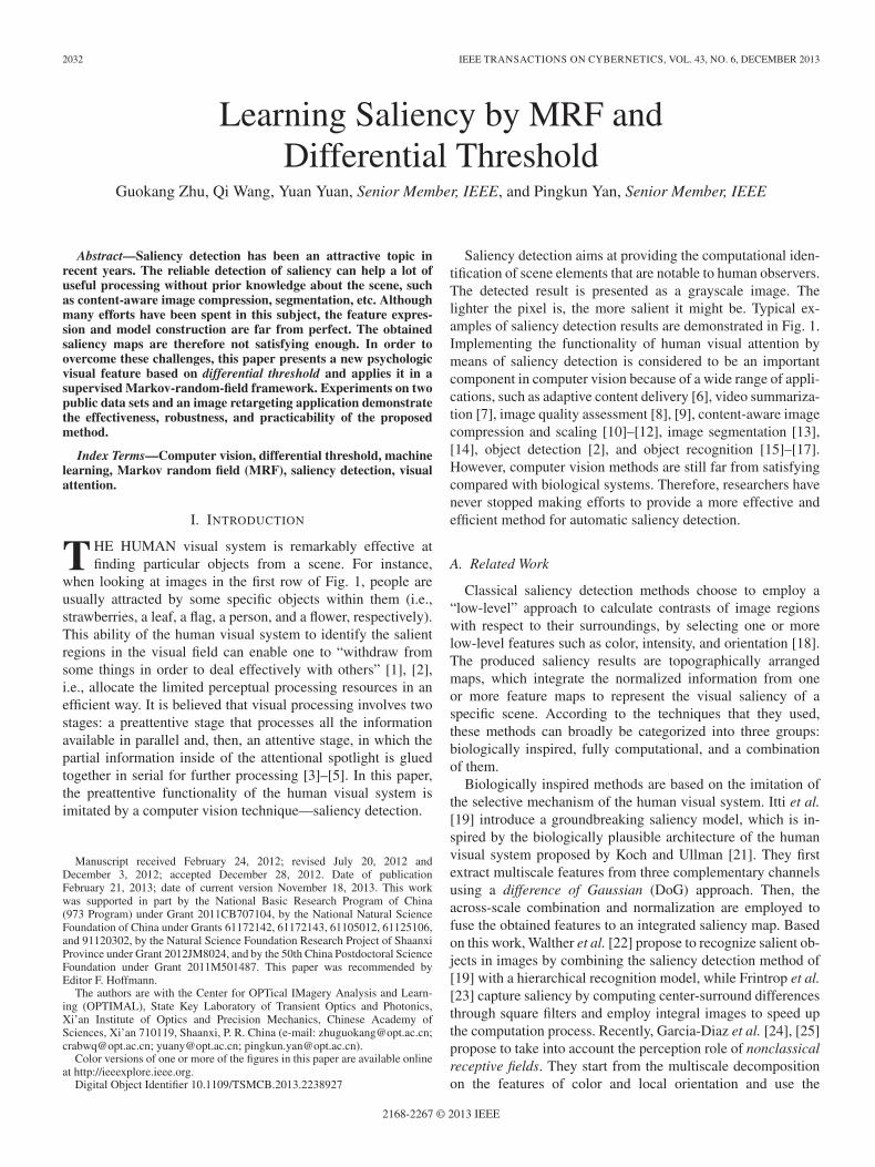
Fig. 4. Statistical map illustrates the saliency distribution for 200 normalizedtraining images. Each pixel in the map indicates the possibility of being salientfor a normalized image with fixed size. The high intensity indicates the highpossibility of a location being salient.

of each color with the weighted feature values of similar colors[measured by (19)]

f(Ii) =∑

Ij∈Mi

w(i, j)f(Ij) (11)

where Mi denotes the m nearest colors of Ii. The weight{w(i, j)}j depends on the difference between the color Ii andIj and satisfies the normalization constraints 0 ≤ w(i, j) ≤ 1and

∑j w(i, j) = 1. More specifically

w(i, j) =1

Z(i)e−D(Ii,Ij)

2/h2

(12)

where Z(i) =∑

j e−D(Ii,Ij)

2/h2is the normalizing factor. The

parameter h controls the decay of the weights as a function ofthe color differences. m and h are experimentally fixed to n/4and 4, respectively, in all our experiments.

C. Center Bias

The center bias is also taken into account due to the fact thathumans naturally put their attentional spotlight near the centerof the image at the first glance, and photographers actually havea bias to make objects of their interest close to the center of thescene. This rule is true for the 200 training images as illustratedin Fig. 4. For these reasons, the proposed method additionallyincludes a feature which indicates the Euclidean distance to thecenter of the image for each pixel.

III. EXPERIMENTS

A. Image Data Set

In order to evaluate the performances of DTMBVS under dif-ferent settings, as well as to compare this method with state-of-the-art saliency detection methods, two publicly available datasets are employed. The first data set containing 1000 images ismanually constructed by Achanta et al. [18] and has achievedgreat popularity in saliency detection [20]. Each of the selectedimage in this data set contains one or several salient objectsand has an accurate object-contour-based ground truth. The

experiments randomly select 200 images and their associatedground truths as the training set and use the remaining 800 asthe testing set. Then, the trained model is further tested on thesecond data set, MSRA-B [34], [35], which contains 5000 well-labeled images, much larger than the first one.

B. Evaluation Measure

In the experiments for quantitative evaluation, the criterioncalled precision-recall curve is chosen to capture the tradeoffbetween accuracy and sensitivity. This parametric curve issketched by varying the threshold used to binarize the saliencymap. Precision measures the rate of the positive detected salientregion to the whole detected region, while recall measures therate of the positive detected salient region to the ground truth.Moreover, F-measure [50], which is a weighted harmonic meanof precision and recall, is also taken to provide a single index.More specifically, given the image with pixels X = {xi} andbinary ground truth G = {gi}, for any detected binary saliencymask L = {li}, these three indexes are defined as

precision =∑i

gili/∑i

li (13)

recall =∑i

gili/∑i

gi (14)

Fα =precision× recall

(1− α)× precision+ α× recall(15)

where α is set to 0.5 according to Martin et al. [50].

C. Color Space Selection

A color space is a model where the independent componentsof color are precisely defined, by which one can quantify,generate, and visualize colors. Different color spaces are suit-able for different applications. Therefore, it is necessary toexperimentally determine the most appropriate color space fora particular task. In this section, six mostly employed colorspaces, CMYK, HSV, RGB, XYZ, YCbCr, and CIELAB, areevaluated on the data set constructed by Achanta et al. to selectthe most suitable one for the proposed method.

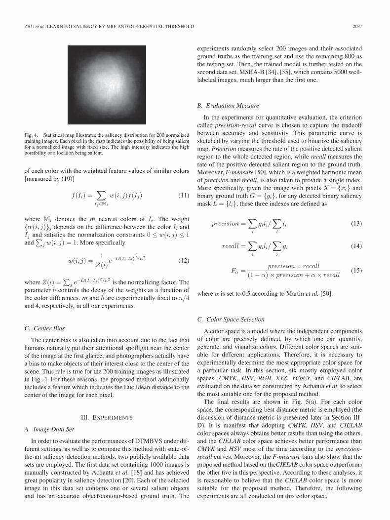
The final results are shown in Fig. 5(a). For each colorspace, the corresponding best distance metric is employed (thediscussion of distance metric is presented later in Section III-D). It is manifest that adopting CMYK, HSV, and CIELABcolor spaces always obtains better results than using the others,and the CIELAB color space achieves better performance thanCMYK and HSV most of the time according to the precision-recall curves. Moreover, the F-measure bars also show that theproposed method based on theCIELAB color space outperformsthe other five in this perspective. According to these analyses, itis reasonable to believe that the CIELAB color space is moresuitable for the proposed method. Therefore, the followingexperiments are all conducted on this color space.


Fig. 5. Precision-recall curves and averaged precision, recall, and F-measure bars of saliency detection results by the proposed method using different settings.(a) Different color spaces. (b) Different color difference measurements in CIELAB color space. “L∗a∗b∗ − L2,” “L∗a∗b∗ − Corr,” “L∗a∗b∗ − L1,” “L∗a∗b∗ −CIEDE,” and “L∗a∗b∗ − ad.L2” are corresponding to (17), (18), (16), CIEDE2000, and (19), respectively. (c) Different color representations. “DTMBVS-HC,”“DTMBVS-FT,” and “DTMBVS-DT” are corresponding to the DTMBVS based on the color representation employed in [18] and [20] and the differentialthreshold-based color representation, respectively. All the experiments are based on the data set constructed by Achanta et al.

D. Color Difference Measurement

Measuring the difference or distance between two colors isan important aspect for color analysis. There are three com-monly used formulas in practical applications [51], [52]. In gen-eral applications, the color difference of two points, I1 and I2,in a full color space is often directly derived from (16) or (17)

D(I1, I2) = ‖I1 − I2‖1 (16)D(I1, I2) = ‖I1 − I2‖2. (17)

The third commonly used formula is based on the concept ofcorrelation coefficient

D(I1, I2) = 1− r(I1, I2) (18)

where r(I1, I2) is the correlation coefficient between I1 and I2.Aside from these three universal formulas, there are also

others designed for specific color spaces. In these formulas, theCIEDE2000 color difference formula has been considered asthe best choice for the CIELAB color metric [53].

It is notable that the aforementioned formulas give the sameweight to each color channel. However, human observers arenot with the equivalent sensibility to the hue, saturation, andlightness changes [54]. Hence, here, the authors propose othercolor difference formulas for the CIELAB (l∗, a∗, b∗) colorspace to match the characteristics of human perception

D(I1, I2) =

√φ (l∗1 − l∗2)

2 + (a∗1 − a∗2)2 + (b∗1 − b∗2)

2 (19)

φ =

{1, if σL∗ ≥ max(σa∗ , σb∗)0, otherwise.

(20)

where σL∗ , σa∗ , and σb∗ are the variances of the correspondingcolor channels.

The biggest difference between the proposed formula andthe previously discussed four equations is that the proposedformula is based on a heuristic perceptual fact that lightnesshas less effect than the color opponent in the visual atten-tion process, unless the lightness variation is large enough.This principle is also improved in our experiments. Fig. 5(b)demonstrates the comparative results. It is manifest that thebest performance is achieved by employing the proposedformula.

E. Effects of Differential Threshold Representation

The proposed DTMBVS contains a differential threshold-based color representation, which aims to imitate the human vi-sual system better while having high computational efficiency.In this section, two relevant color quantization methods [18],[20] are employed to substitute the differential threshold-basedcolor representation. Then, their results are evaluated to verifythe relative advantage of differential threshold.

Fig. 5(c) plots the results of the DTMBVS method basedon different color quantizations. All these curves and barsaltogether can prove that the differential threshold-based colorrepresentation has a clear advantage compared with other ex-isting methods. Therefore, it is reasonable to believe that theproposed color representation is more suitable for the proposedmethod.


Fig. 6. Precision-recall curves of the proposed DTMBVS and state-of-the-art saliency detection methods on (a) data set constructed by Achanta et al. and(b) MSRA-B data set.

F. Comparison With Other Methods

The results of the proposed method are compared with 14state-of-the-art saliency detection methods. They are respec-tively AC [26], AIM [38], AWS [24], [25], CA [33], FT [18],GB [37], HC [20], IM [41], IT [19], LC [49], SEG [32], SeR[30], SR [31], and SUN [39]. These 14 methods are selectedaccording to four certain principles following [18] and [20]:recency (CA, HC, IM, and AWS are proposed during the lasttwo years), high citation frequency (AIM, GB, IT, and SR havebeen cited over 200 times), variety (LC and HC are globalcontrast based; AC, FT, SeR, and SUN are local contrast based;IT and AWS are biologically inspired; and SEG and SR arefully computational), and relation to the proposed DTMBVS(HC and LC). The code for LC is from Cheng et al. [20]. For theother 13 selected methods, their codes are downloaded from theauthors’ home pages. Every method is used to compute saliencymaps for all the testing images. Then, the obtained resultsare compared with the labeled ground truth for quantitativeevaluation.

Fig. 6(a) illustrates the results on the data set constructedby Achanta et al. The precision-recall curves show that theproposed method clearly outperforms AC, AIM, AWS, CA,FT, GB, IM, IT, LC, SEG, SeR, SR, and SUN. The proposedmethod can locate salient regions with much more accuracythan these 13 existing methods, i.e., yield higher precisionwith the same recall rate over the 800-image testing set andvice versa. The proposed method outperforms HC most of thetime, except the disadvantage of lower precision rates when thetasks place more emphasis on achieving extremely high recallrates. However, in practical applications, simply emphasizing

Fig. 7. Averaged precision, recall, and F-measure bars of the proposedDTMBVS and state-of-the-art saliency detection methods on MSRA-Bdata set.

the extremely high recall rate is not a satisfying choice. Abalance between the precision and the recall rate must be moreappropriate [50]. According to this principle, the moderateprecision and recall rates should be referred to. In this case,the proposed method is the best choice in most applications.

In order to further validate the effectiveness and robustnessof the proposed DTMBVS, the MSRA-B image set is alsoemployed in this comparative experiment. The precision-recallresults are presented in Fig. 6(b). It is obvious that DTMBVSoutperforms AC, AIM, FT, HC, IM, IT, LC, SEG, SeR, SR, andSUN on this image set. However, as can be seen in Fig. 6(b),the precision-recall curves cannot provide discriminative clues


Fig. 8. Saliency detection results. From left to right, each column respectively represents the original images, the ground-truth labels, the saliency maps calculatedby AIM [38], AWS [24], [25], CA [33], GB [37], HC [20], IM [41], LC [49], SEG [32], SeR [30], and SUN [39], and the saliency maps calculated by the proposedmethod.

for AWS, CA, and GB. Therefore, the F-measure bars shouldbe taken to provide more discriminative information. The com-parative results are presented in Fig. 7, which shows that theproposed DTMBVS clearly dominates other competitors in theF-measure indicator.

Several visual comparisons are also presented in Fig. 8 forqualitative evaluation. Only the top ten of the 14 aforemen-tioned methods, AIM, AWS, CA, GB, HC, IM, LC, SEG, SeR,and SUN, are selected according to the F-measure indicator tocompare with the proposed one. As can be seen from Fig. 8,the competitive ten methods tend to produce internally incon-gruous or morphological changed salient regions, while theproposed DTMBVS is prone to generate much more consistentresults.

The salient region detected by the proposed method is vis-ibly distinguished with the background. From this result, itcan be inferred that the selected features (i.e., the differentialthreshold-based visual feature and the spatial constraint) canbe more distinguishable than others and the model constructedwith the MRF is more appropriate. Therefore, the proposedmethod has the ability to locate the truly salient regions in agreater probability for each image.

G. Robustness to Noise

Generally, in consideration of the actual conditions, a well-defined model is the one that not only achieves satisfying resultsfor the testing data but also can resist a significant level of noise.In order to evaluate the robustness of all these saliency detectionmethods, a significant level of white Gaussian noise, whichkeeps the SNR = 20 dB, is added to each testing image. Thesecond column of Fig. 9 shows an example image with addednoise. This image is disturbed by numerous white spots. How-ever, the object-background content can still be distinguishedeasily by human eyes.

Fig. 9. First row presents an original image and the corresponding noisyimage. The second row presents the saliency maps calculated by the proposedmethod.

Fig. 10. Performance comparison after adding noise to images. The bars areused to indicate the amounts of changes in the average values of precision,recall, and F-measure. The SNR after adding noise is kept constant at 20 dB.


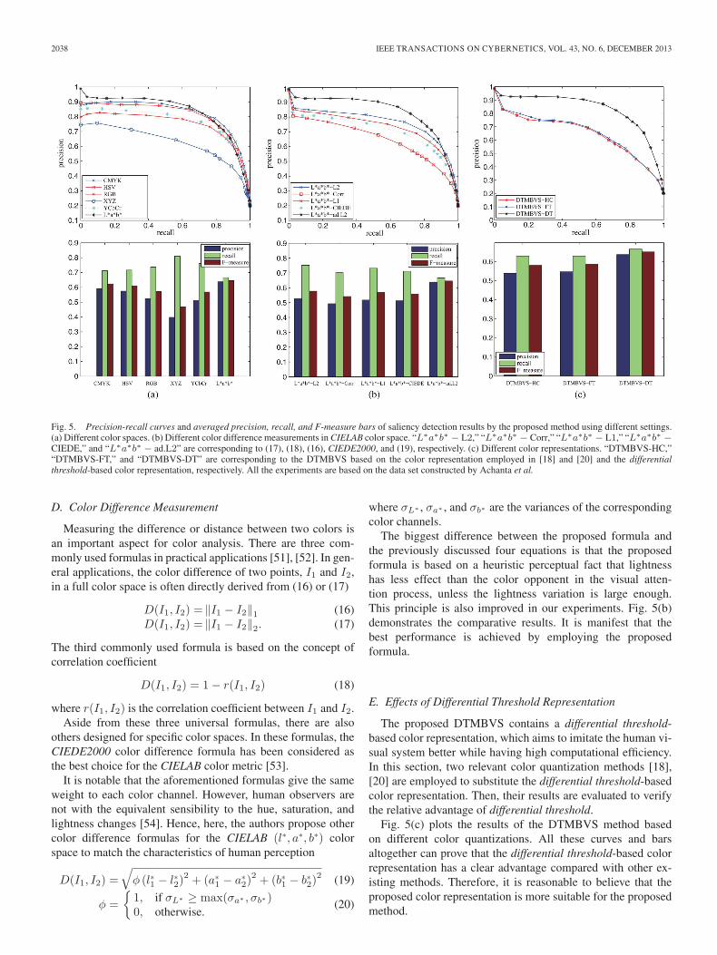
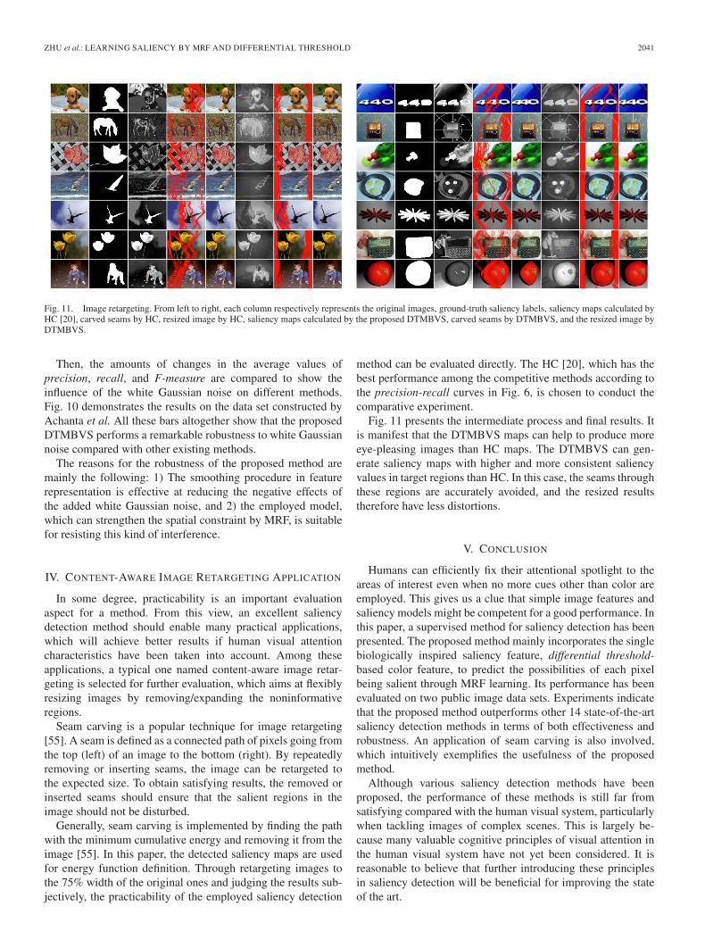
Fig. 11. Image retargeting. From left to right, each column respectively represents the original images, ground-truth saliency labels, saliency maps calculated byHC [20], carved seams by HC, resized image by HC, saliency maps calculated by the proposed DTMBVS, carved seams by DTMBVS, and the resized image byDTMBVS.

Then, the amounts of changes in the average values ofprecision, recall, and F-measure are compared to show theinfluence of the white Gaussian noise on different methods.Fig. 10 demonstrates the results on the data set constructed byAchanta et al. All these bars altogether show that the proposedDTMBVS performs a remarkable robustness to white Gaussiannoise compared with other existing methods.

The reasons for the robustness of the proposed method aremainly the following: 1) The smoothing procedure in featurerepresentation is effective at reducing the negative effects ofthe added white Gaussian noise, and 2) the employed model,which can strengthen the spatial constraint by MRF, is suitablefor resisting this kind of interference.

IV. CONTENT-AWARE IMAGE RETARGETING APPLICATION

In some degree, practicability is an important evaluationaspect for a method. From this view, an excellent saliencydetection method should enable many practical applications,which will achieve better results if human visual attentioncharacteristics have been taken into account. Among theseapplications, a typical one named content-aware image retar-geting is selected for further evaluation, which aims at flexiblyresizing images by removing/expanding the noninformativeregions.

Seam carving is a popular technique for image retargeting[55]. A seam is defined as a connected path of pixels going fromthe top (left) of an image to the bottom (right). By repeatedlyremoving or inserting seams, the image can be retargeted tothe expected size. To obtain satisfying results, the removed orinserted seams should ensure that the salient regions in theimage should not be disturbed.

Generally, seam carving is implemented by finding the pathwith the minimum cumulative energy and removing it from theimage [55]. In this paper, the detected saliency maps are usedfor energy function definition. Through retargeting images tothe 75% width of the original ones and judging the results sub-jectively, the practicability of the employed saliency detection

method can be evaluated directly. The HC [20], which has thebest performance among the competitive methods according tothe precision-recall curves in Fig. 6, is chosen to conduct thecomparative experiment.

Fig. 11 presents the intermediate process and final results. Itis manifest that the DTMBVS maps can help to produce moreeye-pleasing images than HC maps. The DTMBVS can gen-erate saliency maps with higher and more consistent saliencyvalues in target regions than HC. In this case, the seams throughthese regions are accurately avoided, and the resized resultstherefore have less distortions.

V. CONCLUSION

Humans can efficiently fix their attentional spotlight to theareas of interest even when no more cues other than color areemployed. This gives us a clue that simple image features andsaliency models might be competent for a good performance. Inthis paper, a supervised method for saliency detection has beenpresented. The proposed method mainly incorporates the singlebiologically inspired saliency feature, differential threshold-based color feature, to predict the possibilities of each pixelbeing salient through MRF learning. Its performance has beenevaluated on two public image data sets. Experiments indicatethat the proposed method outperforms other 14 state-of-the-artsaliency detection methods in terms of both effectiveness androbustness. An application of seam carving is also involved,which intuitively exemplifies the usefulness of the proposedmethod.

Although various saliency detection methods have beenproposed, the performance of these methods is still far fromsatisfying compared with the human visual system, particularlywhen tackling images of complex scenes. This is largely be-cause many valuable cognitive principles of visual attention inthe human visual system have not yet been considered. It isreasonable to believe that further introducing these principlesin saliency detection will be beneficial for improving the stateof the art.


REFERENCES

[1] W. James, The Principles of Psychology, vol. 1. New York: Henry Holt,1890.

[2] Y. Yu, G. K. I. Mann, and R. G. Gosine, “An object-based visual atten-tion model for robotic applications,” IEEE Trans. Syst., Man, Cybern. B,Cybern., vol. 40, no. 5, pp. 1398–1412, Oct. 2010.

[3] M. I. Posner, J. A. Walker, F. J. Friedrich, and R. D. Rafal, “Effects ofparietal injury on covert orienting attention,” J. Neurosci., vol. 4, no. 7,pp. 1863–1874, Jul. 1984.

[4] A. Belardinelli, F. Pirri, and A. Carbone, “Bottom-up gaze shifts and fixa-tions learning by imitation,” IEEE Trans. Syst., Man, Cybern. B, Cybern.,vol. 37, no. 2, pp. 256–271, Apr. 2007.

[5] A. M. Treisman and S. Sato, “Conjunction search revisited,” J. Exp.Psychol.: Human Percept. Perform., vol. 16, no. 3, pp. 459–478,Aug. 1990.

[6] Y. Ma and H.-J. Zhang, “Contrast-based image attention analysis by usingfuzzy growing,” in Proc. ACM Int. Conf. Multimedia, 2003, pp. 374–381.

[7] S. Marat, M. Guironnet, and D. Pellerin, “Video summarization usinga visual attentional model,” in Proc. Eur. Signal Process. Conf., 2007,pp. 1784–1788.

[8] A. K. Moorthy and A. C. Bovik, “Visual importance pooling for imagequality assessment,” IEEE J. Sel. Topics Signal Process., vol. 3, no. 2,pp. 193–201, Apr. 2009.

[9] J. You, A. Perkis, M. M. Hannuksela, and M. Gabbouj, “Perceptual qualityassessment based on visual attention analysis,” in Proc. ACM Int. Conf.Multimedia, 2009, pp. 561–564.

[10] C. Guo and L. Zhang, “A novel multiresolution spatiotemporal saliencydetection model and its applications in image and video compression,”IEEE Trans. Image Process., vol. 19, no. 1, pp. 185–198, Jan. 2010.

[11] Q. Wang, Y. Yuan, P. Yan, and X. Li, “Saliency detection by multiple-instance learning,” IEEE Trans. Syst., Man, Cybern. B, Cybern., 2012, tobe published.

[12] L. Marchesotti, C. Cifarelli, and G. Csurka, “A framework for visualsaliency detection with applications to image thumbnailing,” in Proc. Int.Conf. Comput. Vis., 2009, pp. 2232–2239.

[13] J. Han, K. N. Ngan, M. Li, and H.-J. Zhang, “Unsupervised extraction ofvisual attention objects in color images,” IEEE Trans. Circuits Syst. VideoTechnol., vol. 16, no. 1, pp. 141–145, Jan. 2006.

[14] C. Jung and C. Kim, “A unified spectral-domain approach for saliencydetection and its application to automatic object segmentation,” IEEETrans. Image Process., vol. 21, no. 3, pp. 1272–1283, Mar. 2012.

[15] U. Rutishauser, D. Walther, C. Koch, and P. Perona, “Is bottom-up atten-tion useful for object recognition,” in Proc. IEEE Int. Conf. Comput. Vis.Pattern Recognit., 2004, pp. II-37–II-44.

[16] L. Yang, N. Zheng, J. Yang, M. Chen, and H. Chen, “A biased samplingstrategy for object categorization,” in Proc. Int. Conf. Comput. Vis., 2009,pp. 1141–1148.

[17] D. Walthera, U. Rutishausera, C. Kocha, and P. Peronaa, “Selective visualattention enables learning and recognition of multiple objects in clutteredscenes,” Comput. Vis. Image Understand., vol. 100, no. 1/2, pp. 41–63,Oct. 2005.

[18] R. Achanta, S. Hemami, F. Estrada, and S. Süsstrunk, “Frequency-tunedsalient region detection,” in Proc. IEEE Int. Conf. Comput. Vis. PatternRecognit., 2009, pp. 1597–1604.

[19] L. Itti, C. Koch, and E. Niebur, “A model of saliency-based visual attentionfor rapid scene analysis,” IEEE Trans. Pattern Anal. Mach. Intell., vol. 21,no. 11, pp. 1254–1259, Nov. 1998.

[20] M. Cheng, G. Zhang, N. J. Mitra, X. Huang, and S. Hu, “Global contrastbased salient region detection,” in Proc. IEEE Int. Conf. Comput. Vis.Pattern Recognit., 2011, pp. 409–416.

[21] C. Koch and S. Ullman, “Shifts in selective visual attention: Towards theunderlying neural circuitry,” Hum. Neurobiol., vol. 4, no. 4, pp. 219–227,1985.

[22] D. Walther, L. Itti, M. Riesenhuber, T. Poggio, and C. Koch, “Attentionalselection for object recognition—A gentle way,” in Proc. Biol. Motiv.Comput. Vis., 2002, pp. 472–479.

[23] S. Frintrop, M. Klodt, and E. Rome, “A real-time visual attention systemusingintegral images,” inProc.Int.Conf.Comput.Vis.Syst.,2007, pp.1–10.

[24] A. Garcia-Diaz, V. Leborán, X. Fdez-Vidal, and X. Pardo, “On the re-lationship between optical variability, visual saliency, and eye fixations:A computational approach,” J. Vis., vol. 12, no. 6, pp. 1–22, Jun. 2012.

[25] A. Garcia-Diaz, X. Fdez-Vidal, X. Pardo, and R. Dosil, “Saliency from hi-erarchical adaptation through decorrelation and variance normalization,”Image Vis. Comput., vol. 30, no. 1, pp. 51–64, Jan. 2012.

[26] R. Achanta, F. J. Estrada, P. Wils, and S. Süsstrunk, “Salient region detec-tion and segmentation,” in Proc. Comput. Vis. Syst., 2008, pp. 66–75.

[27] D. Gao and N. Vasconcelos, “Discriminant saliency for visual recognitionfrom cluttered scenes,” in Proc. Adv. Neural Inf. Process. Syst., 2004,pp. 481–488.

[28] D. Gao and N. Vasconcelos, “Integrated learning of saliency, complexfeatures, and object detectors from cluttered scenes,” in Proc. IEEE Int.Conf. Comput. Vis. Pattern Recognit., 2005, pp. 282–287.

[29] D. Gao, V. Mahadevan, and N. Vasconcelos, “On the plausibility ofthe discriminant center-surround hypothesis for visual saliency,” J. Vis.,vol. 8, no. 7, pp. 1–18, Jun. 2008.

[30] H. J. Seo and P. Milanfar, “Nonparametric bottom-up saliency detectionby self-resemblance,” in Proc. IEEE Int. Conf. Comput. Vis. PatternRecognit., 2009, pp. 45–52.

[31] X. Hou and L. Zhang, “Saliency detection: A spectral residual approach,”in Proc. IEEE Int. Conf. Comput. Vis. Pattern Recognit., 2007, pp. 1–8.

[32] E. Rahtu, J. Kannala, M. Salo, and J. Heikkilä, “Segmenting salient ob-jects from images and videos,” in Proc. Eur. Conf. Comput. Vis., 2010,pp. 366–379.

[33] S. Goferman, L. Zelnik-Manor, and A. Tal, “Context-aware saliency de-tection,” in Proc. IEEE Int. Conf. Comput. Vis. Pattern Recognit., 2010,pp. 2376–2383.

[34] T. Liu, J. Sun, N. Zheng, X. Tang, and H.-Y. Shum, “Learning to detect asalient object,” in Proc. IEEE Int. Conf. Comput. Vis. Pattern Recognit.,2007, pp. 1–8.

[35] T. Liu, Z. Yuan, J. Sun, J. Wang, N. Zheng, X. Tang, and H.-Y. Shum,“Learning to detect a salient object,” IEEE Trans. Pattern Anal. Mach.Intell., vol. 33, no. 2, pp. 353–367, Feb. 2011.

[36] M. Wang, J. Konrad, P. Ishwar, K. Jing, and H. Rowley, “Image saliency:From intrinsic to extrinsic context,” in Proc. IEEE Int. Conf. Comput. Vis.Pattern Recognit., 2011, pp. 417–424.

[37] J. Harel, C. Koch, and P. Perona, “Graph-based visual saliency,” in Proc.Adv. Neural Inf. Process. Syst., 2006, pp. 545–552.

[38] N. Bruce and J. Tsotsos, “Saliency based on information maximization,”in Proc. Adv. Neural Inf. Process. Syst., 2006, pp. 155–162.

[39] L. Zhang, M. H. Tong, T. K. Marks, H. Shan, and G. W. Cottrell, “Sun: ABayesian framework for saliency using natural statistics,” J. Vis., vol. 8,no. 7, pp. 1–20, Dec. 2008.

[40] T. Judd, K. A. Ehinger, F. Durand, and A. Torralba, “Learning to predictwhere humans look,” in Proc. Int. Conf. Comput. Vis., 2009, pp. 2106–2113.

[41] N. Murray, M. Vanrell, X. Otazu, and C. A. Parraga, “Saliency estimationusing a non-parametric low-level vision model,” in Proc. IEEE Int. Conf.Comput. Vis. Pattern Recognit., 2011, pp. 433–440.

[42] S. Baluja, “Using expectation to guide processing: A study of threereal-world applications,” in Proc. Adv. Neural Inf. Process. Syst., 1997,pp. 1–7.

[43] Q. Wang, P. Yana, Y. Yuana, and X. Li, “Multi-spectral saliency detec-tion,” Pattern Recognit. Lett., vol. 34, no. 1, pp. 34–41, Jan. 2013.

[44] Q. Wang, Y. Yuan, P. Yan, and X. Li, “Visual saliency by selectivecontrast,” IEEE Trans. Circuits Syst. Video Technol., vol. 23, no. 7,pp. 1150–1155, Jul. 2013.

[45] J. Shotton, J. Winn, C. Rother, and A. Criminisi, “Texton-boost: Jointappearance, shape and context modeling for multi-class object recognitionand segmentation,” in Proc. Eur. Conf. Comput. Vis., 2006, pp. 1–15.

[46] J. Verbeek and B. Triggs, “Scene segmentation with CRFs learned frompartially labeled images,” in Proc. Adv. Neural Inf. Process. Syst., 2008,pp. 1553–1560.

[47] J. Shotton, A. Blake, and R. Cipolla, “Contour-based learning for objectdetection,” in Proc. Int. Conf. Comput. Vis. Syst., 2005, pp. 503–510.

[48] E. Weber, H. E. Ross, D. J. Murray, and E. H. Weber, On the TactileSenses, 2nd ed. London, U.K.: Psychology Press, 1996.

[49] Y. Zhai and M. Shah, “Visual attention detection in video sequencesusing spatiotemporal cues,” in Proc. ACM Int. Conf. Multimedia, 2006,pp. 815–824.

[50] D. R. Martin, C. Fowlkes, and J. Malik, “Learning to detect natural imageboundaries using local brightness, color, and texture cues,” IEEE Trans.Pattern Anal. Mach. Intell., vol. 26, no. 5, pp. 530–549, May 2004.

[51] A. Gijsenij, T. Gevers, and M. P. Lucassen, “A perceptual comparison ofdistance measures for color constancy algorithms,” in Proc. Eur. Conf.Comput. Vis., 2008, pp. 208–221.

[52] J. Hao, “Human pose estimation using consistent max-covering,” in Proc.IEEE Int. Conf. Comput. Vis. Pattern Recognit., 2010, pp. 1357–1364.

[53] G. Sharma, W. Wu, and E. N. Dalal, “The CIEDE2000 color-differenceformula: Implementation notes, supplementary test data, and mathemati-cal observations,” Color Res. Appl., vol. 30, no. 1, pp. 21–30, Feb. 2005.

[54] H. Y. Lee, H. K. Lee, and Y. H. Ha, “Spatial color descriptor for imageretrieval and video segmentation,” IEEE Trans. Multimedia, vol. 5, no. 3,pp. 358–367, Sep. 2003.

[55] S. Avidan and A. Shamir, “Seam carving for content-aware image resiz-ing,” ACM Trans. Graph., vol. 26, no. 3, pp. 1–10, Jul. 2007.


Guokang Zhu is currently working toward the Ph.D.degree in the Center for Optical Imagery Analysisand Learning, State Key Laboratory of TransientOptics and Photonics, Xi’an Institute of Optics andPrecision Mechanics, Chinese Academy of Sciences,Xi’an, China.

His research interests include computer vision andmachine learning.

Qi Wang received the B.E. degree in automationand the Ph.D. degree in pattern recognition andintelligent system from the University of Scienceand Technology of China, Hefei, China, in 2005 and2010, respectively.

He is currently a Postdoctoral Researcher withthe Center for Optical Imagery Analysis and Learn-ing, State Key Laboratory of Transient Optics andPhotonics, Xi’an Institute of Optics and PrecisionMechanics, Chinese Academy of Sciences, Xi’an,China. His research interests include computer vision

and pattern recognition.

Yuan Yuan (M’05–SM’09) is a Researcher (Full Professor) with the ChineseAcademy of Sciences, Xi’an, China, and her main research interests includevisual information processing and image/video content analysis.

Pingkun Yan (S’04–M’06–SM’10) received theB.Eng. degree in electronics engineering and infor-mation science from the University of Science andTechnology of China, Hefei, China, and the Ph.D.degree in electrical and computer engineering fromthe National University of Singapore, Singapore.

He is a Full Professor with the Center for OpticalImagery Analysis and Learning, State Key Labora-tory of Transient Optics and Photonics, Xi’an In-stitute of Optics and Precision Mechanics, ChineseAcademy of Sciences, Xi’an, China. His research

interests include computer vision, pattern recognition, machine learning, andtheir applications in medical imaging.

Learning Saliency by MRF and Differential Threshold Learning Saliency by MRF and... · Learning Saliency by MRF and Differential Threshold Guokang Zhu, Qi Wang, Yuan Yuan, Senior

Documents