Lead, zinc, and chromium concentrations in acidic headwater streams in Sweden explained by chemical, climatic, and land-use variations

Biogeosciences, 9, 4323–4335, 2012www.biogeosciences.net/9/4323/2012/doi:10.5194/bg-9-4323-2012© Author(s) 2012. CC Attribution 3.0 License.

Biogeosciences

Lead, zinc, and chromium concentrations in acidic headwaterstreams in Sweden explained by chemical, climatic, and land-usevariations

B. J. Huser, J. Folster, and S. J. Kohler

Department of Aquatic Sciences and Assessment, Swedish University of Agricultural Sciences, Sweden

Correspondence to:B. J. Huser ([email protected])

Received: 28 December 2011 – Published in Biogeosciences Discuss.: 14 February 2012Revised: 9 October 2012 – Accepted: 11 October 2012 – Published: 7 November 2012

Abstract. Long-term data series (1996–2009) for elevenacidic headwater streams (< 10 km2) in Sweden were ana-lyzed to determine factors controlling concentrations of tracemetals. In-stream chemical data as well climatic, flow, anddeposition chemistry data were used to develop models pre-dicting concentrations of chromium (Cr), lead (Pb), and zinc(Zn). Data were initially analyzed using partial least squaresto determine a set of variables that could predict metal con-centrations across all sites. Organic matter (as absorbance)and iron related positively to Pb and Cr, while pH relatednegatively to Pb and Zn. Other variables such as conduc-tivity, manganese, and temperature were important as well.Multiple linear regression was then used to determine mini-mally adequate prediction models which explained an aver-age of 35 % (Cr), 52 % (Zn), and 72 % (Pb) of metal variationacross all sites. While models explained at least 50 % of vari-ation in the majority of sites for Pb (10) and Zn (8), onlythree sites met this criterion for Cr. Investigation of varia-tion between site models for each metal revealed geographi-cal (altitude), chemical (sulfate), and land-use (silvaculture)influences on predictive power of the models. Residual anal-ysis revealed seasonal differences in the ability of the mod-els to predict metal concentrations as well. Expected futurechanges in model variables were applied and results showedthe potential for long-term increases (Pb) or decreases (Zn)for trace metal concentrations at these sites.

1 Introduction

Trace metals are naturally present in atmospheric, terrestrialand aquatic environments; however, anthropogenic impactshave affected availability and cycling greatly. Efforts in un-derstanding processes controlling mobility of trace metalsin running waters are increasing with implementation of theEuropean Water Framework Directive, especially given thatsuch understanding is critical for assessing potential impactsfrom metals on the hydrosphere and in separation of natu-ral and anthropogenic impacts on availability and variabil-ity. While rivers with large, generally urban catchments orpolluted streams have been well studied, headwater streamshave received less attention, especially with respect to metalschemistry.

Headwaters are an important resource for biodiversity andhuman welfare (Lowe and Likens, 2005; Bishop et al., 2008),mainly because they cover a substantial portion of the water-course length, providing a large proportion of water and so-lutes to downstream sites (Alexander et al., 2007). This is es-pecially true in Sweden where streams with catchment sizesless than 10 km2 make up approximately 90 % of the totallength of all perennial watercourses (Bishop et al., 2008). Itis widely known that variability in water quality is relatedto catchment size, with small catchment watercourses typi-cally showing the highest variability in both space (Wolock etal., 1997; Temnerud and Bishop, 2005) and time (Nagorski etal., 2003; Buffam et al., 2007). Significant efforts have beenmade to quantify the variability of headwaters (Rawlins etal., 1999; Likens and Buso, 2006), but few studies discussingtrace metals in Scandinavian headwaters have been published

Published by Copernicus Publications on behalf of the European Geosciences Union.

4324 B. J. Huser et al.: Lead, zinc and chromium in Swedish streams

even though the boreal Northern Hemisphere is rich in thesetypes of systems.

Cycling of trace metals is complex because many factorsinfluence metal behavior including biotic and abiotic chem-ical processes, hydrology, climate, land use and the proper-ties of the metals themselves. A general regulator of mobil-ity, pH affects the solubility of many metal ions. However,other factors can affect the mobility and transport of metalsto and within surface water systems. Organic matter (OM)mineralization and chemical processes (e.g. changes in ionicstrength) can alter metal solubility and mobility (Landre etal., 2009; Porcal et al., 2009). The form of metal (e.g. dis-solved, colloidal, or particulate) may also be an importantfactor when describing temporal variation of metal concen-trations (e.g. lead (Pb) and zinc (Zn)) in surface waters (Sher-rell and Ross, 1999; Ross and Sherrell, 1999). The differentfactors affecting trace metal mobility may explain confound-ing evidence of increasing metals (e.g. Pb) in some streams inSweden (Huser et al., 2011) even as deposition of metals hasbeen decreasing since the 1970s (Ruhling and Tyler, 2004).

The aim of this study is to determine factors that can pre-dict trace metal mobility in small, acidic headwater streamsin Sweden. In-stream chemical, climatic, and land-use char-acteristics likely affect trace metal concentrations together orseparately, depending on the metal and its specific reactivity.Although metal mobility may relate to numerous factors, weattempt to explain variability using a few dominant variables.A unique long-term chemical data series (1996–2009) for thestreams is available and used to develop predictive modelsdescribing changes in chromium (Cr), Pb, and Zn concentra-tions in these streams. Site specific models are then comparedto large-scale chemical, land-use, climatic and geographicvariables to determine if differences in explanatory powerof the models can be explained. Predicted future changes inmetal concentrations, based on recent trends in model vari-ables, are discussed as well.

2 Methods

2.1 Study area

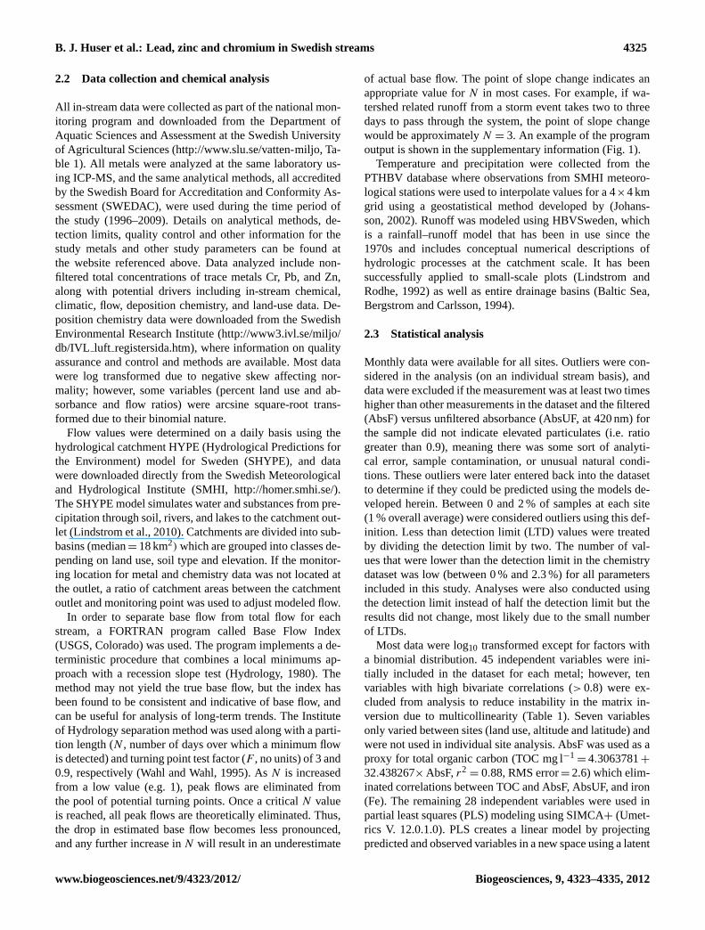
The streams included in this study are situated across Sweden(Fig. 1) and the data time series ranged from 1996 through2009. Only monitoring sites that were not directly influencedby point sources (e.g. wastewater treatment plants, mining fa-cilities, industrial plants, etc.) were included in the analysis.This initial group of monitoring sites totaled 139 streams thatwere included in a study to determine long-term trends formetals in streams and rivers in Sweden (Huser et al., 2011).From these sites, streams that had a maximum catchmentsize of 10 km2 and a median pH value less than 6.0 were se-lected (11 sites) because metals generally tend to be mostlyin the dissolved form under these conditions (Kohler, 2010;Sjostedt et al., 2009).

28

Figure 1. Stream sites and the limes norrlandicus boundary separating Sweden into northern and southern climactic regions.

Fig. 1.Stream sites and thelimes norrlandicusboundary separatingSweden into northern and southern climactic regions.

To further analyze data spatially, the country was dividedinto two regions based on the “limes norrlandicus” ecotonewhich divides Sweden into a southern nemoral and boreo-nemoral zone and a northern boreal and alpine zone (Fig. 1).Climate also varies between the regions with the major dif-ference, outside of ecosystem type, being that the southernregion is warmer than the northern region. Thus, thelimesnorrlandicusrepresents the approximate boundary separat-ing areas where flow is low during winter with pronouncedsnowmelt in spring (the north) and flow is more or less con-tinuous during the year with little to no accumulation of snowduring winter (south).

Biogeosciences, 9, 4323–4335, 2012 www.biogeosciences.net/9/4323/2012/

B. J. Huser et al.: Lead, zinc and chromium in Swedish streams 4325

2.2 Data collection and chemical analysis

All in-stream data were collected as part of the national mon-itoring program and downloaded from the Department ofAquatic Sciences and Assessment at the Swedish Universityof Agricultural Sciences (http://www.slu.se/vatten-miljo, Ta-ble 1). All metals were analyzed at the same laboratory us-ing ICP-MS, and the same analytical methods, all accreditedby the Swedish Board for Accreditation and Conformity As-sessment (SWEDAC), were used during the time period ofthe study (1996–2009). Details on analytical methods, de-tection limits, quality control and other information for thestudy metals and other study parameters can be found atthe website referenced above. Data analyzed include non-filtered total concentrations of trace metals Cr, Pb, and Zn,along with potential drivers including in-stream chemical,climatic, flow, deposition chemistry, and land-use data. De-position chemistry data were downloaded from the SwedishEnvironmental Research Institute (http://www3.ivl.se/miljo/db/IVL luft registersida.htm), where information on qualityassurance and control and methods are available. Most datawere log transformed due to negative skew affecting nor-mality; however, some variables (percent land use and ab-sorbance and flow ratios) were arcsine square-root trans-formed due to their binomial nature.

Flow values were determined on a daily basis using thehydrological catchment HYPE (Hydrological Predictions forthe Environment) model for Sweden (SHYPE), and datawere downloaded directly from the Swedish Meteorologicaland Hydrological Institute (SMHI,http://homer.smhi.se/).The SHYPE model simulates water and substances from pre-cipitation through soil, rivers, and lakes to the catchment out-let (Lindstrom et al., 2010). Catchments are divided into sub-basins (median= 18 km2) which are grouped into classes de-pending on land use, soil type and elevation. If the monitor-ing location for metal and chemistry data was not located atthe outlet, a ratio of catchment areas between the catchmentoutlet and monitoring point was used to adjust modeled flow.

In order to separate base flow from total flow for eachstream, a FORTRAN program called Base Flow Index(USGS, Colorado) was used. The program implements a de-terministic procedure that combines a local minimums ap-proach with a recession slope test (Hydrology, 1980). Themethod may not yield the true base flow, but the index hasbeen found to be consistent and indicative of base flow, andcan be useful for analysis of long-term trends. The Instituteof Hydrology separation method was used along with a parti-tion length (N , number of days over which a minimum flowis detected) and turning point test factor (F , no units) of 3 and0.9, respectively (Wahl and Wahl, 1995). AsN is increasedfrom a low value (e.g. 1), peak flows are eliminated fromthe pool of potential turning points. Once a criticalN valueis reached, all peak flows are theoretically eliminated. Thus,the drop in estimated base flow becomes less pronounced,and any further increase inN will result in an underestimate

of actual base flow. The point of slope change indicates anappropriate value forN in most cases. For example, if wa-tershed related runoff from a storm event takes two to threedays to pass through the system, the point of slope changewould be approximatelyN = 3. An example of the programoutput is shown in the supplementary information (Fig. 1).

Temperature and precipitation were collected from thePTHBV database where observations from SMHI meteoro-logical stations were used to interpolate values for a 4×4 kmgrid using a geostatistical method developed by (Johans-son, 2002). Runoff was modeled using HBVSweden, whichis a rainfall–runoff model that has been in use since the1970s and includes conceptual numerical descriptions ofhydrologic processes at the catchment scale. It has beensuccessfully applied to small-scale plots (Lindstrom andRodhe, 1992) as well as entire drainage basins (Baltic Sea,Bergstrom and Carlsson, 1994).

2.3 Statistical analysis

Monthly data were available for all sites. Outliers were con-sidered in the analysis (on an individual stream basis), anddata were excluded if the measurement was at least two timeshigher than other measurements in the dataset and the filtered(AbsF) versus unfiltered absorbance (AbsUF, at 420 nm) forthe sample did not indicate elevated particulates (i.e. ratiogreater than 0.9), meaning there was some sort of analyti-cal error, sample contamination, or unusual natural condi-tions. These outliers were later entered back into the datasetto determine if they could be predicted using the models de-veloped herein. Between 0 and 2 % of samples at each site(1 % overall average) were considered outliers using this def-inition. Less than detection limit (LTD) values were treatedby dividing the detection limit by two. The number of val-ues that were lower than the detection limit in the chemistrydataset was low (between 0 % and 2.3 %) for all parametersincluded in this study. Analyses were also conducted usingthe detection limit instead of half the detection limit but theresults did not change, most likely due to the small numberof LTDs.

Most data were log10 transformed except for factors witha binomial distribution. 45 independent variables were ini-tially included in the dataset for each metal; however, tenvariables with high bivariate correlations (> 0.8) were ex-cluded from analysis to reduce instability in the matrix in-version due to multicollinearity (Table 1). Seven variablesonly varied between sites (land use, altitude and latitude) andwere not used in individual site analysis. AbsF was used as aproxy for total organic carbon (TOC mg l−1

= 4.3063781+32.438267× AbsF,r2

= 0.88, RMS error= 2.6) which elim-inated correlations between TOC and AbsF, AbsUF, and iron(Fe). The remaining 28 independent variables were used inpartial least squares (PLS) modeling using SIMCA+ (Umet-rics V. 12.0.1.0). PLS creates a linear model by projectingpredicted and observed variables in a new space using a latent

www.biogeosciences.net/9/4323/2012/ Biogeosciences, 9, 4323–4335, 2012

4326 B. J. Huser et al.: Lead, zinc and chromium in Swedish streams

Table 1.Variable information and % missing values (from a total of1689). All data are log transformed except pH and where indicated(∗).

Variable Description Unit % missing

Abs∗f/uf Filtered/unfiltered Abs 0.0AbsF Filtered absorbance 420 nm/5 cm 0.0AbsUF∗∗ Unfiltered absorbance 420 nm/5 cm 0.0Al Total aluminum µg l−1 0.8Alk∗∗ Alkalinity meq l−1 0.1Alt Altitude m above sea level 0.0BF∗ Baseflow m3 s−1 0.0BF/F∗ Baseflow/total flow 0.0Ca∗∗ Calcium meq l−1 0.0Cl∗∗ Chloride meq l−1 0.3Cond Conductivity mS/m25 0.0Cr Chromium µg l−1 28.6F Fluoride mg l−1 0.3Fe Iron µg l−1 2.0Flow Total flow m3 s−1 0.7Forest∗ Forest % total area 0.0K Potassium meq l−1 0.3Mg Magnesium meq l−1 0.0Mn Manganese µg l−1 2.8Na∗∗ Sodium meq l−1 0.0NH4 Ammonia µg l−1 0.0NO2NO3 Nitrate–nitrite µg l−1 0.0Pb Lead µg l−1 13.9pH pH 0.0Precip Precipitation Mm 0.7Runoff Runoff Mm 0.4Si Silica mg l−1 0.0Silva∗ Harvested area % total area 0.0SO4 Sulfate meq l−1 0.4Temp Temperature K 0.0TN Total nitrogen µg l−1 0.0TOC∗∗ Total organic carbon mg l−1 20.4Total Area Watershed area km2 0.0TP Total phosphorus µg l−1 0.1Water∗ Surface water area % total area 0.0Wetland∗ Wetland area % total area 0.0Y Latitude 0.0Zn Zinc µg l−1 14.5

Parameters measured in direct precipitation

H+ Hydrogen µeq m−2 16.9Cl∗∗ Chloride mg m−2 16.0NO3∗∗ Nitrate mg m−2 16.4SO4 Sulfate mg m−2 16.0NH4∗∗ Ammonia mg m−2 16.1Ca Calcium mg m−2 16.2Mg Magnesium mg m−2 16.5Na∗∗ Sodium mg m−2 16.2K Potassium mg m−2 16.2Cond∗∗ Conductivity mS m−1 16.1

∗Arcsine square-root transformed.∗∗Removed due to multicollinearilty (correlation factor> 0.8).

variable approach to model the covariance structure betweentwo matrices (X and Y) and maximize the correlation be-tweenX andY variables. PLS was used as an initial step to

reduce the number of parameters used in multiple linear re-gression (MLR) modeling based on the variable importancefor the projection (VIP). VIP values are calculated for eachindependent variable by summing the squares of the PLSweights, which are weighted by the amount of the dependentvariable explained in the model. A set of common variableswas determined by including terms that had strong predic-tion effects (VIP> 0.9) in more than 50 % of the individualPLS site models. This group of terms was then used in MLRanalysis.

After reducing the number of independent variables viaPLS, MLR analysis was performed, and a single, minimallyadequate model (common model) with greater generality wasdeveloped for all sites. Dominant variables were substitutedinto the model until the average of individual site variancesexplained increased by less than two percent (all values asadjustedr2). After common models were developed for eachmetal, residual analysis was conducted to detect potentialoutliers, extreme values or other factors that could bias theresults of model fitting. The common model for each metalwas then applied to the entire dataset, and expected futurechanges in model variables were applied to predict futureconcentrations of each metal. The modeling scheme usedherein, from PLS to MLR analysis, is described graphicallyin supplementary Fig. S1.

3 Results

The sites included in this study (Fig. 1) were generally com-parable in terms of water chemistry and land use (Table 2).Median trace metal concentrations (Table 3) varied betweenstreams but were less variable than other in-stream parame-ters, with minimum to maximum ratios of 2.8, 5.2, and 4.5for median Cr, Pb, and Zn, respectively. In total, 28 indepen-dent variables were used in the modeling process with resultsdescribed below.

3.1 PLS Analysis

PLS analysis was conducted to determine which of the inde-pendent variables were most strongly related to each metal.Variables at this level of analysis included in-stream chem-ical, deposition, flow, and climatic data (Table 1). To de-termine if factors such as suspended particles or flow con-ditions might influence the results strongly, PLS analysiswas conducted on the entire dataset for each metal usingtwo conditions which set limitations on the data included inthe analysis, including only low suspended particulate matter(AbsF/AbsUF> 0.9, 66 % of total data) and only low runoffor base flow dominated periods (base flow/total flow> 0.9,64 % of total data). In some cases, PLS models with lim-ited data decreased in predictive power when compared tomodels using all data. If a model did improve, however, ex-plained variation generally increased by less than 5 % (data

Biogeosciences, 9, 4323–4335, 2012 www.biogeosciences.net/9/4323/2012/

B. J. Huser et al.: Lead, zinc and chromium in Swedish streams 4327

Table 2.Selected site parameters (medians), land use (% area), estimated anthropogenic acidification (1pH) since 1860, and future expectedrecovery (1pH future) for each stream by 2030, except where no data (ND) is indicated.

Name Area (km2) pH 1pH 1pH future Cond (mS cm−1) SO2−

4 (meq l−1) TOC (mg l−1) Fe (µg l−1) Wetland Open Water Forest Harvested Other

Aneboda IM 0.19 4.51 −1.22 +0.11 5.8 0.147 18.7 910 15 14 54 5 11Bratangsbacken 5.75 4.73 −1.55 −0.07 3.4 0.068 16.8 600 7 2 85 7 0Gammtratten IM 0.52 5.64 −0.23 +0.03 1.7 0.042 7.5 357 1 0 99 0 0Kindlahojden IM 0.24 4.58 −1.46 +0.14 3.1 0.107 7.4 292 0 0 100 0 0Kvarnebacken 6.98 5.18 −1.26 +0.12 3.6 0.066 9.9 410 12 6 78 4 0Lill-F amtan 5.95 4.79 −0.36 +0.03 1.7 0.034 9.6 355 5 3 91 0 1Lommabacken Nedre 1.06 4.43 ND ND 3.7 0.070 16.1 455 3 4 92 0 0Pipbacken Nedre 1.35 4.78 −1.25 −0.02 5.2 0.100 7.9 989 37 3 51 9 0Ringsmobacken 1.82 4.40 ND ND 4.4 0.055 12.6 315 15 5 77 3 0Sagebacken 4.40 4.87 −1.17 +0.03 4.6 0.073 15.5 960 13 4 72 9 1Svartberget 1.94 5.13 −0.64 +0.01 2.9 0.091 19.8 1200 20 2 74 4 0

not shown). Thus, the entire dataset was used for modelingpurposes for each metal.

PLS modeling by individual site for Cr, Pb, and Zn showedvarying importance for the 28 variables used in the study.Of the most dominant variables with VIP scores> 0.9 (Ta-ble 4), AbsF and aluminum (Al) related positively to allmetals while sulfate (SO4) related negatively. Temperature(Temp) was also a dominant variable that related positively toCr concentrations but was mixed (positively and negativelyrelated) for Pb and Zn. Pb and Zn were negatively related topH while Cr and Pb were positively related to Fe. Cr was neg-atively related to nitrate–nitrite (NO2NO3) and Zn was pos-itively related to conductivity (Cond). These variables andothers listed in Table 4 were used in MLR analysis detailedbelow.

3.2 Multivariate linear regression analysis

MLR analysis for Pb included 8 terms (dominant variableswith VIP > 0.9) from the initial PLS analysis. Site spe-cific MLR resulted in a common model including AbsF, Fe,and pH (Fig. 2) with ten of the eleven sites having greaterthan 50 % of variance explained (Table 5). Two examplesof model fit for monitoring data are provided in Fig. 3.Ringsmobacken (r2

= 0.40) was the only site that did notfollow the general pattern detected at the other sites. Nocombination of independent variables (all 35 were tested)could explain more than 50 % of the variation for Pb atRingsmobacken. Investigation of residuals of model fit forthe common model revealed a distinct break in the datasetbeginning in 2007 where residuals skewed to the negativeand residual variance decreased substantially. While varianceexplained in the data improved somewhat when the com-mon model was applied only to data before 2007 (r2

= 0.44),it improved substantially when applied to data from 2007–2009 (r2

= 0.66). Investigation into sampling methods forthis site revealed that a change in sampling personnel oc-curred in late 2006, which may be responsible for the dif-fering results.

The initial MLR model for Zn included 11 terms with VIPscores> 0.9 in the PLS analysis (Table 4). Development ofthe common model (Fig. 2) from site specific MLR analy-

sis resulted in three dominant terms (pH, Cond, Mn) andprovided generally good explanation (> 50 %) of variabil-ity in Zn for eight of the eleven sites (Table 5). Similar toPb, analysis of model fit for Ringsmobacken revealed a dis-tinct change beginning in 2007 when overall model variancedecreased and residuals were no longer centered but nega-tively skewed. Common model application to the split timeseries revealed no improvement to model fit from 1996–2005(r2

= 0.24) but substantial improvement when the model wasapplied to more recent data from 2007–2009 (r2

= 0.59).Aneboda IM, a site just downstream from a wetland that wasalso poorly described by the common model (r2

= 0.01), didnot show any obvious long-term temporal changes through-out the time series but appeared to be affected by seasonalchanges in flow. Analysis of the common model residualsby month (data not shown) revealed better model fit duringMarch and April, months typically with higher flow due tospring melt. Additional residual analysis confirmed this withhigher flows generally resulting in lower model residuals.

MLR analysis for Cr included 11 terms (VIP> 0.9) frominitial PLS modeling. Although there were 11 variables thatwere present in at least 50 % of the PLS site models, the stan-dard errors for VIP factors were generally much higher thanfor Zn or Pb (Table 4), indicating higher variability in theability of the variables to predict Cr concentrations. In con-trast to Pb and Zn, site specific MLR models were gener-ally poor at explaining variations in Cr concentrations in the11 streams. The common model (Table 5) explained greaterthan 50 % of variance at only three of the eleven sites (35 %average). Due to the low predictive power of the commonmodel, all 28 variables were included in a second attemptusing MLR to find an adequate model, but no increase inthe variance explained was found and the original variablesused above remained the best possible factors for the com-mon model.

3.3 Variation in model predictive power by site andseason

Investigation of the differences in variability explained be-tween site models revealed chemical, climatic, geograph-ical, and land-use effects on site model predictive power.

www.biogeosciences.net/9/4323/2012/ Biogeosciences, 9, 4323–4335, 2012

4328 B. J. Huser et al.: Lead, zinc and chromium in Swedish streams

Table 3.Metal concentrations (medians and 10th and 90th percentiles) for each study stream.

Stream Zn Pb Cr Zn Pb Cr(µg l−1) (µg l−1) (µg l−1) 10th, 90th Percentiles

Aneboda IM 3.2 0.72 0.53 2.4, 7.8 0.46, 1.80 0.31, 0.89Bratangsbacken 6.2 0.57 0.41 5.2, 7.8 0.44, 0.86 0.33, 0.56Gammtratten IM 1.9 0.18 0.22 1.2, 3.0 0.12, 0.29 0.17, 0.31Kindlahojden IM 8.0 0.38 0.23 5.7, 10 0.30, 0.60 0.20, 0.32Kvarnebacken 6.5 0.56 0.36 5.5, 8.1 0.43, 0.67 0.25, 0.54Lill-F amtan 4.1 0.71 0.21 3.0, 6.2 0.48, 1.10 0.13, 0.30Lommabacken Nedre 6.8 0.62 0.37 5.8, 8.2 0.50, 0.76 0.28, 0.45Pipbacken Nedre 8.2 0.52 0.33 5.6, 11 0.27, 1.54 0.14, 0.58Ringsmobacken 8.5 0.94 0.41 5.8, 16 0.63, 1.41 0.28, 0.52Sagebacken 7.4 0.91 0.59 6.0, 9.2 0.55, 1.39 0.43, 0.83Svartberget 2.5 0.44 0.48 1.6, 3.7 0.31, 0.67 0.33, 0.64

Medians of the values used in the initial PLS models (exclud-ing the variables making up the common models) along withland-use and geographical data were used in MLR regres-sion to determine if any relationships could be found withinvariance explained (r2) between the sites. Relationships be-tween model variance explained and SO4 and harvested area(both positively correlated) for Pb (r2

= 0.87) and Si and al-titude (positively and negatively correlated, respectively) forCr (r2

= 0.81) were detected (Fig. 4). No pattern for modelpredictive power between sites was detected for Zn.

To determine seasonal variability in predictive power ofthe common models, means of the model residuals werecompared by month (Fig. 5). Residuals for Pb gener-ally skewed negatively during the fall and winter seasons(September through December), while Zn model residualsskewed negatively from November through February. BothZn and Pb model residuals were positively skewed from latespring into the summer months. Residuals for Cr showed notrend by season.

4 Discussion

PLS was used to screen 28 chemical, flow, deposition chem-istry, and climatic variables to develop a set of dominantvariables for use in MLR analysis to develop common mod-els describing variation in Cr, Pb and Zn in small-catchmentacidic streams in Sweden. Common models were developedfor the three metals by analyzing site specific data and thenapplied to the dataset as a whole.

4.1 Parameters controlling metal concentrations

Mobility and form of all metals in this study are affectedby stream chemistry (to varying degrees). Because the studystreams were acidic, the fractionation of the total metals islikely to be dominated by the dissolved form, especially forZn. The strongest chemical predictors were organic matter(AbsF) and pH, and it is well known that that these two pa-

Table 4. Dominant independent variables (present in more than50 % of PLS site models) with VIP factors> 0.9. N = number ofsites where model variable was included and, SE= VIP standarderror.

Cr Pb ZnN VIP SE N VIP SE N VIP SE

AbsF 9 1.8 0.53 11 2.0 0.24 7 1.4 0.28Al 9 1.6 0.76 11 1.6 0.30 9 1.6 0.38Cond 7 1.2 0.77 9 1.6 0.38Fe 11 1.9 0.43 11 1.9 0.33Flow 6 1.1 0.25K 8 1.3 0.49 6 1.2 0.31Mg 6 1.3 0.88 7 1.4 0.27Mn 7 1.2 0.44 10 1.5 0.42NO2NO3 7 1.1 0.70pH 7 1.2 0.37 10 1.5 0.35Runoff 6 1.0 0.26SO4 10 1.4 0.52 8 1.4 0.24 9 1.3 0.32Temp 9 1.2 0.48 8 1.1 0.29 7 1.2 0.25TN 6 1.2 0.81TP 6 1.5 0.45 7 1.3 0.36

rameters are related to trace metal mobility in surface waters.Cr, Pb, and Zn have been shown to interact strongly withdissolved organic carbon (DOC) or TOC in streams (Lan-dre et al., 2009; Gundersen and Steinnes, 2003), generallyincreasing overall mobility. AbsF appears to control muchof the within site variation for Pb (and to a lesser extentCr), correlating positively to metal concentration. Both pH(negatively correlated) and Fe (positively correlated) werealso important components in the common model for Pb.The strong relationship between Pb and Fe and AbsF is notunexpected as others have shown similar results (Pokrovskyand Schott, 2002) and organo-metallic complexation is a wellknown phenomenon (e.g. Weng et al., 2002). However, Tip-ping et al. (2002) suggested that Fe (as well as Al) can actas a competitor with metals for common binding sites onOM. Wallstedt et al. (2010) instead postulated that increas-ing Fe-colloid formation was responsible, at least in part,

Biogeosciences, 9, 4323–4335, 2012 www.biogeosciences.net/9/4323/2012/

B. J. Huser et al.: Lead, zinc and chromium in Swedish streams 4329

29

Figure 2. Variables included in each common model for Pb (A), Zn (B, Aneboda removed), and Cr (C). Box plots are shown with medians, 25 and 75th quantiles and 10 and 90% quantiles (whiskers).

pH Absf Fe Absf, pH Absf, pH, Fe

r2

0.0

0.2

0.4

0.6

0.8

1.0A

pH Cond Mn pH, Cond pH, Cond, Mn

r2

0.0

0.2

0.4

0.6

0.8

1.0B

T Fe Abs Fe, Absf Fe, Absf, T

r2

0.0

0.2

0.4

0.6

0.8

1.0C

Fig. 2.Variables included in each common model for Pb(A), Zn (B)(Aneboda IM removed), and Cr(C). Box plots are shown with me-dians, 25 and 75th quantiles, and 10 and 90 % quantiles (whiskers).

for increasing trace metal concentrations (i.e. V and As) instreams across southern Sweden. While Fe was a dominantfactor among site models, it explained only 8 % additionalvariation (average across site models) in Pb concentration af-ter pH and AbsF were added to the model (64 % of variationexplained). However, the importance of Fe varied across sitesand was positively correlated to the Fe / TOC (or AbsF) ra-tio in the streams. Thus, while Fe was of lesser importancewhen predicting Pb variation across sites, on average, it be-came more important as the Fe / TOC ratio increased above0.04.

30

Figure 3. Monitored and modeled data for Zn and Pb from selected sites. Data originally excluded fom analysis as outliers are shown as well.

0

0.5

1

1.5

2

2.5

3

1995 1996 1997 1998 1999 2000 2001 2002 2003 2004 2005 2006 2007 2008 2009 2010

Pb C

once

ntra

tion

(ug

L-1)

Kindlahöjden IM

Monitoring DataCommon ModelOutliers

0

1

2

3

4

5

6

7

8

1995 1996 1997 1998 1999 2000 2001 2002 2003 2004 2005 2006 2007 2008 2009 2010

Zn C

once

ntra

tion

(ug

L-1)

Svartberget

Fig. 3. Monitored and modeled data for Pb and Zn from Kind-lahojden IM (A) and Svartberget(B), respectively. Data originallyexcluded from analysis as outliers are shown as well.

The weaker relationship (relative to AbsF) between Pb andpH supports other studies showing that effects of acidifica-tion are relatively minor in comparison to changes in DOCwith respect to Pb transport (Neal et al., 1997; Tipping etal., 2003). This was not the case for all sites in this study.For example, if pH and AbsF at Pipbacken Nedre (medianpH 4.7) increased by 10 % and 20 %, respectively, Pb con-centrations would be expected to decrease by approximately4.1 %. If we take a look at a less acidic site (Svartberget, me-dian pH 5.1), however, the same increase in pH and AbsFresults in an increase (12 %) in average Pb concentration.Although this is a hypothetical scenario, it appears that invery acidic streams pH exerts more influence on Pb concen-trations, while at higher pH (but still acidic) organic matterexerts more control. In support of this, data for filtered andunfiltered metal concentrations at 24 stream sites in Sweden(including five of the sites included herein) showed 85 to100 % of Pb detected was in dissolved form at pH values lessthan 4.8 (Kohler, 2010). From pH 4.8 to pH 6.0, dissolvedPb was as low as 39 % of the total concentration, indicatingorganic or colloid bound Pb fractions were more dominant.Thus, when the total concentration of Pb was dominated bythe dissolved form when pH was near 4.8 (or less), pH had

www.biogeosciences.net/9/4323/2012/ Biogeosciences, 9, 4323–4335, 2012

4330 B. J. Huser et al.: Lead, zinc and chromium in Swedish streams

31

Figure 4. Actual variance explained by the common model or each site versus predicted variance based on SO4 and Silva (Pb) or Si and Alt (Cr). Ringsmobäcken was excluded from the analysis.

Fig. 4. Actual variance explained by the common model or eachsite versus predicted variance based on SO4 and Silva (Pb) or Siand altitude (Cr). Ringsmobacken was excluded from the analysis.

a greater effect on Pb concentrations because colloidal andparticulate fractions were likely low.

The most common variables determined for Zn with PLSanalysis were pH (10 sites), Mn (10 sites) and Cond (9 sites).pH was negatively related to Zn, while Cond and Mn werepositively related. Other factors not included in the final com-mon model included Fe and Al (significant factor at 9 sites).While Zn has been shown to bind with OM in freshwaters,the affinity of Zn for binding sites is lower than that found forother metals (Bergkvist et al., 1989). In addition, Zn is gener-ally found in mostly dissolved form under a wide range of pHvalues (Gundersen and Steinnes, 2003), including streams inSweden (Kohler, 2010). Thus, total Zn concentrations in thestudy streams are likely dominated by the dissolved fractionand the fact that pH explains a large amount of Zn varia-tion in these streams is not surprising. The strong positiverelationship between Cond and Zn concentrations is also notsurprising given that metal solubility is positively related toionic strength of a solution (Helz et al., 1975). Mn, nearly asimportant for the common model as Cond, is more difficultto explain but may relate to Zn concentrations in a numberof ways. Zn tends to solubilize under both low pH and redoxconditions (Sims and Patrick, 1978). Mn, being redox sensi-tive, may be an indicator of low redox conditions and is gen-erally first to become reduced compared to a number of otherpotential electron acceptors (Mn> NO3- > Fe> SO2−

4 ). Insupport of this is the inverse relationship between Mn con-centrations of both flow and runoff at eight of eleven sites,indicating greater chance for low redox conditions and Mnreduction under low flow conditions. However, the positiverelationship between Mn and Zn could also be a dilution ofgroundwater inputs containing Mn and Zn (Carpenter andHayes, 1978) under high flow conditions, but it is difficultto discern the true nature of the relationship between thesetwo elements without additional data (i.e. redox or ground-water input). MnO2 dissolution and release of adsorbed Zncould be expected with decreasing pH, but Mn and pH ap-

32

Figure 5. Model residuals (untransformed, excluding Aneboda for Zn) by month for Pb (A) and Zn (B).

0 1 2 3 4 5 6 7 8 9 10 11 12 13

Pb

resi

dual

/Pb

conc

.

-0.6

-0.4

-0.2

0.0

0.2

0.4

0.6 A

Month

0 1 2 3 4 5 6 7 8 9 10 11 12 13

Zn re

sidu

al/Z

n co

nc.

-0.6

-0.4

-0.2

0.0

0.2

0.4

0.6B

Fig. 5.Model residuals (untransformed, excluding Aneboda IM forZn) by month for Pb(A) and Zn(B).

pear to operate independently, at least in these streams, be-cause there was no general relationship detected between thetwo variables.

Only three of the eleven sites were adequately describedby the common model for Cr. The chemistry of Cr is com-plex due to multiple oxidation states, the potential effects ofstream chemistry, and interactions with both organic and in-organic constituents. Another factor that may limit the un-derstanding of Cr in these streams is the prevalence of rela-tively low Cr concentrations. The median values for Cr at thestudy sites are considered either low or very low for Sweden(Swedish EPA, 1999), and it can be difficult to generalizeoverall processes driving Cr concentrations at these levels.Analytical variability may overwhelm natural in-stream vari-ation at low concentrations, making determination of control-ling processes difficult. Nonetheless, at the three sites wheregreater than 50 % of variance was explained, either AbsFand/or Fe were significant, positively correlated factors inthe common model. These three sites also had the smallestcatchments in the study (between 0.19 and 0.52 km2). Forlarger catchments including a high percentage of surface wa-ter (e.g. lakes), the controlling mechanisms for Cr may be

Biogeosciences, 9, 4323–4335, 2012 www.biogeosciences.net/9/4323/2012/

B. J. Huser et al.: Lead, zinc and chromium in Swedish streams 4331

more complex. Reduction of Cr (VI) to the less mobile Cr(III) is generally favored in systems with higher organic mat-ter (Bartlett, 1991), and Cr (III) tends to be more stable at lowpH (Richard and Bourg, 1991). Organic matter (e.g. DOC),however, has been shown to increase the pH range of solubil-ity for Cr (III) in laboratory tests (Remoundaki et al., 2007).Increasing temperature, the final term in the common model,has been shown to lead to increases in DOC (Dalva andMoore, 1991), potentially increasing solubility of Cr. How-ever, given the poor explanatory power of the model, it isdifficult to generalize about factors that control Cr concen-trations in these streams.

4.2 Common model applied to all data

The common model developed by assessing dominant factorsacross individual site models was applied to the entire datasetfor each metal. Results were similar when comparing the av-erager2 of the individual site common models for Zn andCr to the common model applied to all data (Table 5). Thecomparison for Pb, however, was substantially different withthe common model, underperforming when applied to thedataset as a whole. Variability in predictive power betweenPb site models was explained well (r2

= 0.86,p = 0.001) bymedian sulfate concentration and Silva (Fig. 4), with no otherparameters significantly (p < 0.05) contributing to variabil-ity explained. The relationship between sulfate and predictivepower of the models likely represents an acidification sig-nal, with variability explained increasing as median sulfateincreases. Erlandsson et al. (2008) showed TOC concentra-tions in some Swedish streams were driven partly by SO2−

4 ,which may indicate that Pb concentrations in areas affectedby anthropogenic acidification would be better predicted us-ing a model including organic matter. Three sites with someof the lowestr2 values (excluding Ringsmobacken) wereall located north of thelimes norrlandicusdivide (Fig. 1)and receive less sulfate deposition than stations located fur-ther south (Ruhling and Tyler, 2004), supporting the impor-tance of SO4 in model performance. Silva was also positivelycorrelated with model variance explained and may indicatechanges in degradation and mobility (or type) of organic mat-ter and associated Pb (Vuori et al., 2003).

Variability in predictive power for Zn models could notbe explained between sites (with or without Aneboda IMbeing included), likely meaning that the relationship of thecommon model variables to Zn between sites is less affectedby large-scale differences (e.g. land use, climate, etc.). Thesimilarity between average variability explained by site andvariability explained in the entire dataset using the commonmodel seems to support this. Variability in Cr site model pre-dictive power was explained well (r2

= 0.81,p = 0.0031) bydifferences in median Si (positively correlated, 55 %) and al-titude (negatively correlated, 26 %). Further interpretation isnot presented, however, due to the overall poor performanceof the common model.

4.3 Seasonal variability

Median model residuals by month for Pb and Zn were gen-erally close to zero, but some seasonal patterns were de-tected (Fig. 5). Model residuals for Pb skewed negatively inthe fall to early winter period (September–December), mean-ing the model overpredicts the actual Pb concentration in thestreams. This time of year is generally wetter, especially insouthern Sweden, with decreasing temperatures. While wet-ter conditions can increase the transport of carbon to streams(Erlandsson et al., 2008), the data for study sites herein showthe opposite with higher flow and runoff correlating to lowerAbsF (or TOC). The type of OM exported to the streams dur-ing this period may affect Pb transport and mobility, but noinformation exists in the dataset to assess this hypothesis.Residuals skewed to the positive and variability increasedduring summer months, which are typically drier and baseflow tends to be a larger portion of the total flow. Both me-dian AbsF and Fe increase (by almost a factor of two) dur-ing summer at these sites, while pH increases to a lesser ex-tent (0.2 units). Reduced transport of watershed sources ofPb along with varying types of OM present (e.g. greater au-tochthonous production) would likely lead to overpredictionby the model (negative residuals), which is not the case here.Because Pb and Zn residuals were generally similar, espe-cially during the summer low flow period, we theorize thatsome process or processes not included in the models may beresponsible. One possible explanation for positive residualsfor both Pb and Zn during summer may be resuspension ofsediments under low flow conditions. Median AbsF/AbsUFvalues were lowest (i.e. higher particulates) during summerunder low flow conditions, and wind or sampling activitymay have disturbed bottom sediments during sample collec-tion. An alternative explanation may be that the higher per-centage of groundwater in the streams (base flow/total flowwas highest during summer) led to a relatively higher amountof solutes in the streams. Without additional data on metalpartitioning, however, it is difficult to speculate further onthe reasons behind the similar seasonal trends for Pb and Znresiduals.

4.4 Model applicability to peak values and outliers

Model variance was equally distributed compared to depen-dent variable concentrations, and thus models were able topredict values close to the mean as well as peak or extremevalues for Pb and Zn. In cases where a number of peak val-ues (but not by definition outliers, as indicated in the meth-ods) for any of the metals were present at a site, these val-ues were excluded (whether model fit was good for thesepoints or not) and MLR analysis was conducted again todetermine if these values disproportionally influenced theamount of variability explained in the model. For example,three elevated values for Pb (between 1.14 and 1.76 µg l−1)

at Kindlahojden (median Pb= 0.38 µ g l−1) were excluded

www.biogeosciences.net/9/4323/2012/ Biogeosciences, 9, 4323–4335, 2012

4332 B. J. Huser et al.: Lead, zinc and chromium in Swedish streams

Table 5.Step-wise multiple linear regression models and variance explained (r2) by site and using all data. Statistically significant variablesare shown in order of importance (absolute value of the t-ratio).

Name Pb∗ Zn∗∗ Cr∗∗∗

r2 Terms r2 Terms r2 Terms

Aneboda IM 0.93 AbsF, pH 0.01 0.75 FeBratangsbacken 0.85 AbsF, Fe, pH 0.59 Mn, C, pH 0.26 FeGammtratten IM 0.54 Fe, pH 0.56 pH, Mn, C 0.74 Fe, TKindlahojden IM 0.84 AbsF, pH, Fe 0.75 C, pH 0.70 AbsFKvarnebacken 0.70 Fe, pH 0.54 C, Mn 0.13 Fe, AbsFLill-F amtan 0.59 AbsF, pH, Fe 0.45 Mn, C, pH 0.15 Fe, TLommabacken Nedre 0.62 AbsF, pH 0.56 Mn, C, pH 0.16 FePipbacken Nedre 0.88 AbsF, pH, Fe 0.59 C, pH 0.33Ringsmobacken 0.40 pH, AbsF, Fe 0.24 Mn, pH 0.07 FeSagebacken 0.79 Fe, AbsF 0.74 C, Mn, pH 0.24 FeSvartberget 0.77 AbsF, pH, Fe 0.66 pH, Mn, C 0.31 Fe, T, AbsF

Average 0.72 0.52 0.35All data† 0.52 0.55 0.35

∗Pb model terms: Fe, AbsF, pH.∗∗Zn model terms: pH, Cond (C), Mn.∗∗∗Cr model terms: Fe, AbsF, Temp (T).†Model applied to all data available for each metal instead of by individual site

and the amount of variation explained decreased somewhatbut remained high (r2 of 0.83 versus 0.93). Of the oth-ers sites for Pb where extreme values were removed (Ane-boda IM, Pibacken Nedre), decrease in variation explainedwas low (less than 5 %) or a slight increase was detected(Sagebacken). When MLR analysis was conducted after peakremoval for Zn at three sites where elevated peaks were de-tected (Aneboda IM, Ringsmobacken, Sagebacken), varia-tion explained improved although only marginally (< 5 %)at each site. The analysis of the common models for Pb andZn shows that the variables are able to predict not only valuesnear the median but peak or extreme values near an order ofmagnitude higher than the median for both metals.

The models were also applied to outliers that were re-moved from the dataset before analysis began. One data pointfor Pb was removed as an outlier from the original dataset forKindlahojden IM before analysis. When this value was en-tered back into the dataset (Fig. 3), the common model under-predicted the actual value by 38 % and the value had a z-score(number of standard deviations from the mean) higher than 3,indicating it is likely an outlier as originally suspected. OneZn data point was removed from the dataset for Svartberget(Fig. 3), and when it was included, the common model pre-diction was within 8.6 % of the actual value. Even though theZn concentration had a z-score (z = 4.6) higher than 3, thisvalue is probably not an outlier, at least based on the commonmodel developed for Zn.

4.5 Past trends and future changes in metalconcentrations

Many of the variables included in the common models de-veloped for Pb and Zn have shown long-term, consistentchanges in the past and are likely to continue to change in thefuture. According to Moldan et al. (2004), pH values have in-creased (from the 1970s) and are expected to increase furtherin many acidified systems in Sweden over the next 20 yr dueto reduced deposition of acidifying compounds. Althoughthe study by Moldan et al. (2004) focuses on lakes, similartrends were also found for streams in Sweden (Folster andWilander, 2002). Based on these data, at least seven of theeleven streams included in our study appear to be acidifiedrelative to 1860 (Table 2), and pH is expected to increaseover the next 20 yr. DOC levels have generally increased inSweden from 1990–2004 (Monteith et al., 2007) and maycontinue to do so in the future. In a large-scale study (139streams across Sweden), Huser et al. (2011) showed long-term (1996–2009) increasing trends for pH, Fe, and TOC,and decreasing trends for conductivity in streams and riversin Sweden. Because the study by Huser et al. (2011) includedstreams in our study, the long-term trends were used to es-timate future changes in common model variables to pre-dict potential changes in Pb and Zn (Table 6) in 10 sitesincluded in this study (excluding Ringsmobacken). Trendsfor all Pb and Zn model variables (except Mn) were avail-able. Using Theil slopes (% change year-1) from the Huser etal. (2011) trend data, all sites showed decreasing Zn concen-trations caused by increasing pH and/or decreasing conduc-tivity. Three of these sites (Kindlahojden IM, Lill-Famten,

Biogeosciences, 9, 4323–4335, 2012 www.biogeosciences.net/9/4323/2012/

B. J. Huser et al.: Lead, zinc and chromium in Swedish streams 4333

Table 6. Predicted changes (1% total) in Pb and Zn during thenext 20 yr based on previous long-term trends (1996–2009, Huseret al., 2011) for common model variables (pH, TOC, Fe, and Cond),shown as % change per year (%1 yr−1). TOC was used as a proxyfor AbsF. Aneboda IM was excluded from Zn analysis (NA) due tolow model power. NT= no significant trend detected.

1 % yr−1 1 % totalStream pH TOC Fe Cond Pb Zn

Aneboda IM 0.28 NT 1.9 −2.0 −5.1 NABratangsbacken 0.34 2.3 3.5 −2.1 31.7 −21.4Gammtratten IM 0.27 NT NT NT −9.1 −21.9Kindlahojden IM† 0.36 2.0 2.6 −3.4 1.3 −78.7Kvarnebacken NT NT 2.0 NT 10.0 0.0Lill-F amtan† 0.34 3.1 4.1 −2.7 30.5 −43.3Lommabacken Nedre 0.30 3.1 3.3 −2.3 28.0 −20.9Pipbacken Nedre∗† 0.58 NT NT −2.3 −4.1 −30.1Sagebacken NT NT 1.8 NT 18.8 0.0Svartberget∗ NT 3.5 NT −2.3 57.3 −16.7

† Decreasing Zn trends (1996–2009) from Huser et al. (2011).∗ Increasing (Svartberget) or decreasing (Pipbacken Nedre) Pb trends (1996–2009) from Huseret al. (2011).

and Pipbacken Nedre) were previously shown to have de-creasing trends in Zn concentration from 1996–2009 (Huseret al., 2011). These three sites also had the greatest 20-yr pre-dicted future changes in Zn (greater than 1.5 % yr−1) basedon the common model developed in this study.

Pb concentrations are expected to increase over the next20 yr (1.3 to 57.3 %) based on trend data for pH, Fe, andTOC (used as a proxy for AbsF,r2

= 0.88); however, themodel results showed decreasing concentrations for threeof the sites. These sites either had significant trends onlyfor pH (Gammtratten IM, Pipbacken Nedre) or had a rela-tively low median pH (Aneboda IM) compared to the othersites. As discussed previously, it appears that in very acidicstreams (i.e. median pH< 5), pH likely exerts a greater effecton Pb concentration compared with other parameters due tothe high amounts of non-colloidal dissolved Pb. Sites previ-ously shown to have long-term decreasing (Pipbacken Ne-dre) or increasing (Svartberget) trends (Huser et al., 2011)showed similar trends for expected future changes in Pb con-centrations based on the common model developed herein.Although we show expected future trends for Zn and Pb, careshould be taken when interpreting the results because the ex-trapolation of future changes in model variables is based onrecent trends (1996–2009) that may or may not continue intothe future.

5 Summary

Long-term data series (1996–2009) for eleven acidic smallcatchment streams in Sweden were analyzed to develop pre-dictive models able to explain variability for trace metal con-centrations. Models developed for Pb (pH, AbsF, Fe) and Zn(pH, Cond, Mn) explained more than 50 % of metal varia-

tion for most sites, whereas the model developed for Cr waspoor and further explanation into potential drivers was notpossible. The dependence of Pb on the model variables wasnot surprising, given that others have shown similar resultsfor other types of water courses. On the other hand, OMhas previously been shown to control Zn mobility, but de-scribed little to no variation in Zn concentrations and wasnot included in the common model. This is probably due, atleast in part, to the acidic nature of the study streams. Modelvariance was equally distributed compared to the dependentvariable concentrations, and thus models were able to predictvalues close to the mean as well as peak or extreme valuesfor Pb and Zn. In some cases, when suspected outliers wereadded back in to the dataset, it appeared they were naturallyhigh values and model fit was good whereas in other casesthey were likely outliers probably caused by contamination,laboratory error, or some other problem. Model variance didvary slightly by season, indicating changes in factors suchas flow regime, sediment resuspension, or DOC mobility andtype may alter the prediction level of the models, and furtherresearch into the mechanisms behind these seasonal differ-ences is warranted. When model parameters were adjusted toreflect potential future scenarios for variables such as AbsF,pH, and Cond, both increases (Pb) and decreases (Zn) weregenerally seen for the streams included in this study. The re-sults are able to explain the sometimes confounding evidencebetween decreasing metals deposition over the past 30 yr andincreasing concentrations for metals like Pb in some streamsin Sweden, and may be useful for predicting future problemsrelating to issues such as toxicity and water quality standardsfor metals in this region.

Supplementary material related to this article isavailable online at:http://www.biogeosciences.net/9/4323/2012/bg-9-4323-2012-supplement.pdf.

Acknowledgements.The authors thank the many people atthe laboratory for the Department for Aquatic Sciences andAssessment, SLU, who collected and analyzed the substantialamount of samples in this study. Roger Herbert, Louise Bjorkvald,and Teresia Wallstedt were instrumental in developing a largeportion of the database that was used as part of this study.We also thank the Swedish Environmental Protection Agency forfunding much of the collection and analysis of the samples and data.

Edited by: J. Kesselmeier

References

Alexander, R. B., Boyer, E. W., Smith, R. A., Schwarz, G. E.,and Moore, R. B.: The role of headwater streams in down-stream water quality, J. Am. Water Resour. As., 43, 41–59,doi:10.1111/j.1752-1688.2007.00005.x, 2007.

www.biogeosciences.net/9/4323/2012/ Biogeosciences, 9, 4323–4335, 2012

4334 B. J. Huser et al.: Lead, zinc and chromium in Swedish streams

Bartlett, R. J.: Chromium Cycling in Soils and Water - Links, Gaps,and Methods, Environ. Health Persp., 92, 17–24, 1991.

Bergkvist, B., Folkeson, L., and Berggren, D.: Fluxes of Cu, Zn, Pb,Cd, Cr, and Ni in Temperate Forest Ecosystems - a Literature-Review, Water Air Soil Poll., 47, 217–286, 1989.

Bergstrom, S. and Carlsson, B.: River Runoff to the Baltic Sea –1950–1990, Ambio, 23, 280–287, 1994.

Bishop, K., Buffam, I., Erlandsson, M., Folster, J., Laudon, H.,Seibert, J., and Temnerud, J.: Aqua Incognita: the unknown head-waters, Hydrol. Process., 22, 1239–1242,doi:10.1002/Hyp.7049,2008.

Buffam, I., Laudon, H., Temnerud, J., Morth, C. M., and Bishop, K.:Landscape-scale variability of acidity and dissolved organic car-bon during spring flood in a boreal stream network, J. Geophys.Res.-Biogeo., 112, G01022,doi:10.1029/2006jg000218, 2007.

Carpenter, R. H. and Hayes, W. B.: Precipitation of iron, man-ganese, zinc, and copper on clean, ceramic surfaces in a streamdraining a polymetallic sulfide deposit, J. Geochem. Explor., 9,31–37,doi:10.1016/0375-6742(78)90036-5, 1978.

Dalva, M. and Moore, T. R.: Sources and Sinks of DissolvedOrganic-Carbon in a Forested Swamp Catchment, Biogeochem-istry, 15, 1–19, 1991.

Erlandsson, M., Buffam, I., Folster, J., Laudon, H., Temnerud, J.,Weyhenmeyer, G. A., and Bishop, K.: Thirty-five years of syn-chrony in the organic matter concentrations of Swedish rivers ex-plained by variation in flow and sulphate, Global Change Biol.,14, 1191–1198,doi:10.1111/j.1365-2486.2008.01551.x, 2008.

Folster, J. and Wilander, A.: Recovery from acidification in Swedishforest streams, Environ. Pollut., 117, 379–389, 2002.

Gundersen, P. and Steinnes, E.: Influence of pH and TOC concen-tration on Cu, Zn, Cd, and Al speciation in rivers, Water Res., 37,307–318,doi:10.1016/s0043-1354(02)00284-1, 2003.

Helz, G. R., Huggett, R. J., and Hill, J. M.: Behavior of Mn, Fe, Cu,Zn, Cd and Pb Discharged from a Wastewater Treatment Plantinto an Estuarine Environment, Water Res., 9, 631–636, 1975.

Huser, B. J., Kohler, S. J., Wilander, A., Johansson, K., and Folster,J.: Temporal and spatial trends for trace metals in streams andrivers across Sweden (1996–2009), Biogeosciences, 8, 1813–1823,doi:10.5194/bg-8-1813-2011, 2011.

Johansson, B.: Estimation of areal precipitation for hydrologicalmodelling in Sweden, Ph.D., Earth Science Centre, GoteborgUniversity, Goteborg, 2002.

Kohler, S.: Comparing filtered and unfiltered metal concentrationsin some swedish surface waters, Department of Aquatic Sciencesand Assessment, Uppsala, 59 pp., 2010.

Landre, A. L., Watmough, S. A., and Dillon, P. J.: The effectsof dissolved organic carbon, acidity and seasonality on metalgeochemistry within a forested catchment on the PrecambrianShield, central Ontario, Canada, Biogeochemistry, 93, 271–289,doi:10.1007/s10533-009-9305-0, 2009.

Likens, G. E. and Buso, D. C.: Variation in streamwater chemistrythroughout the Hubbard Brook Valley, Biogeochemistry, 78, 1–30,doi:10.1007/s10533-005-2024-2, 2006.

Lindstrom, G. and Rodhe, A.: Transit Times of Water in SoilLysimeters from Modeling of O-18, Water Air Soil Poll., 65, 83–100, 1992.

Lindstrom, G., Pers, C., Rosberg, J., Stromqvist, J., and Arheimer,B.: Development and testing of the HYPE (Hydrological Predic-tions for the Environment) water quality model for different spa-

tial scales, Hydrol. Res., 41, 295–319,doi:10.2166/Nh.2010.007,2010.

Lowe, W. H. and Likens, G. E.: Moving headwater streams to thehead of the class, Bioscience, 55, 196–197, 2005.

Moldan, F., Kronnas, V., Wilander, A., Karltun, E., and Cosby, B.J.: Modelling acidification and recovery of swedish lakes, WaterAir Soil Poll., 4, 139–160, 2004.

Monteith, D. T., Stoddard, J. L., Evans, C. D., de Wit, H. A.,Forsius, M., Hogasen, T., Wilander, A., Skjelkvale, B. L., Jef-fries, D. S., Vuorenmaa, J., Keller, B., Kopacek, J., and Vesely,J.: Dissolved organic carbon trends resulting from changesin atmospheric deposition chemistry, Nature, 450, 537–539,doi:10.1038/Nature06316, 2007.

Nagorski, S. A., Moore, J. N., McKinnon, T. E., and Smith,D. B.: Scale-dependent temporal variations in streamwater geochemistry, Environ Sci Technol, 37, 859–864,doi:10.1021/Es025983+, 2003.

Neal, C., Robson, A. J., Jeffery, H. A., Harrow, M. L., Neal, M.,Smith, C. J., and Jarvie, H. P.: Trace element inter-relationshipsfor the Humber rivers. Inferences for hydrological and chemicalcontrols, Sci. Total Environ., 194, 321–343, 1997.

Pokrovsky, O. S. and Schott, J.: Iron colloids/organic matter associ-ated transport of major and trace elements in small boreal riversand their estuaries (NW Russia), Chem. Geol., 190, 141–179,doi:10.1016/s0009-2541(02)00115-8, 2002.

Porcal, P., Koprivnjak, J. F., Molot, L. A., and Dillon, P. J.: Humicsubstances-part 7: the biogeochemistry of dissolved organic car-bon and its interactions with climate change, Environ. Sci. Pollut.R., 16, 714–726,doi:10.1007/s11356-009-0176-7, 2009.

Rawlins, B. G., Smith, B., Hutchins, M. G., and Lister, T. R.: Tem-poral and spatial variability in stream waters of Wales, the Welshborders and part of the West Midlands, UK – 2. Alumino-silicatemineral stability, carbonate and gypsum solubility, Water Res.,33, 3492–3502, 1999.

Remoundaki, E., Hatzikioseyian, A., and Tsezos, M.: A sys-tematic study of chromium solubility in the presence of or-ganic matter: consequences for the treatment of chromium-containing wastewater, J. Chem. Technol. Biot., 82, 802–808,doi:10.1002/jctb.1742, 2007.

Richard, F. C. and Bourg, A. C. M.: Aqueous geochem-istry of chromium: A review, Water Res., 25, 807–816,doi:10.1016/0043-1354(91)90160-r, 1991.

Ross, J. M. and Sherrell, R. M.: The role of colloids in tracemetaltransport and adsorption behavior in New Jersey Pinelandsstreams, Limnol. Oceanogr., 44, 1019–1034, 1999.

Ruhling, A. and Tyler, G.: Changes in the atmospheric deposition ofminor and rare elements between 1975 and 2000 in south Swe-den, as measured by moss analysis, Environ. Pollut., 131, 417–423,doi:10.1016/j.envpol.2004.03.005, 2004.

Sherrell, R. M. and Ross, J. M.: Temporal variability of trace metalsin New Jersey Pinelands streams: Relationships to discharge andpH, Geochim. Cosmochim. Ac., 63, 3321–3336, 1999.

Sims, J. L. and Patrick, W. H.: Distribution of micronutrient cationsin soil under conditions of varying redox potential and pH, SoilSci. Soc. Am. J., 42, 258–262, 1978.

Sjostedt, C., Wallstedt, T., Gustafsson, J. P., and Borg, H.:Speciation of aluminium, arsenic and molybdenum in ex-cessively limed lakes, Sci. Total Environ., 407, 5119–5127,doi:10.1016/j.scitotenv.2009.05.034, 2009.

Biogeosciences, 9, 4323–4335, 2012 www.biogeosciences.net/9/4323/2012/

B. J. Huser et al.: Lead, zinc and chromium in Swedish streams 4335

Swedish EPA: Bedomningsgrunder for miljokvalitet. Sjoar och vat-tendrag. Kemiska och fysikaliska parametrar., Naturvardsverket,Stockholm4920, 205 pp., 1999.

Temnerud, J. and Bishop, K.: Spatial variation of streamwaterchemistry in two Swedish boreal catchments: Implications forenvironmental assessment, Environ. Sci. Technol., 39, 1463–1469, 2005.

Tipping, E., Rey-Castro, C., Bryan, S. E., and Hamilton-Taylor,J.: Al(III) and Fe(III) binding by humic substances in freshwa-ters, and implications for trace metal speciation, Geochim. Cos-mochim. Ac., 66, 3211–3224, 2002.

Tipping, E., Rieuwerts, J., Pan, G., Ashmore, M. R., Lofts, S.,Hill, M. T. R., Farago, M. E., and Thornton, I.: The solid-solution partitioning of heavy metals (Cu, Zn, Cd, Pb) in up-land soils of England and Wales, Environ. Pollut., 125, 213–225,doi:10.1016/S0269-7491(03)00058-7, 2003.

Vuori, K. M., Siren, O., and Luotonen, H.: Metal contamination of

streams in relation to catchment silvicultural practices: a compar-ative study in Finnish and Russian headwaters, Boreal. Environ.Res., 8, 61–70, 2003.

Wahl, K. L. and Wahl, T. L.: Determining the flow of Comel Springsat New Braunfels, Texas, Texas Water ’95, San Antonio, Texas,16–17 August 1995, 1995.

Wallstedt, T., Bjorkvald, L., and Gustafsson, J. P.: Increas-ing concentrations of arsenic and vanadium in (south-ern) Swedish streams, Appl. Geochem., 25, 1162–1175,doi:10.1016/j.apgeochem.2010.05.002, 2010.

Weng, L. P., Temminghoff, E. J. M., Lofts, S., Tipping, E., and VanRiemsdijk, W. H.: Complexation with dissolved organic matterand solubility control of heavy metals in a sandy soil, Environ.Sci. Technol., 36, 4804–4810,doi:10.1021/Es0200084, 2002.

Wolock, D. M., Fan, J., and Lawrence, G. B.: Effects of basin sizeon low-flow stream chemistry and subsurface contact time inthe Neversink River Watershed, New York, Hydrol. Process., 11,1273–1286, 1997.

www.biogeosciences.net/9/4323/2012/ Biogeosciences, 9, 4323–4335, 2012